Effect of Mold Contour on Interfacial Heat Transfer During Solidification of AlSi11Cu3Fe Alloy (ADC-12)

Abstract

The present work investigated the effect of flat, concave, and convex mold contours on heat transfer during the solidification of an aluminum AlSi11Cu3Fe (ADC-12) alloy. Experiments were designed with copper/steel cylindrical and flat molds to study the effect of convex and flat casting/mold interface on heat transfer. To examine the effect of a concave and flat interfaces, an experimental setup consisting of a cylindrical and square bar chill was fabricated. Casting/mold (chill) interfacial heat flux was estimated by solving an inverse heat conduction problem (IHCP). The temperatures measured at locations inside the mold/chill were used as input to the inverse solver. It was observed that the flat contour yielded higher heat flux than a convex contour for both copper and steel molds. Although the volume to surface area (V/A) ratio for castings solidified against a flat and convex interface are the same, the larger mold volume associated with the flat interface yielded higher heat flux transients. Experiments involving chills suggested that the flat interface resulted in higher heat transfer when the (V/A) ratio for the chill was the same. To study and compare the combined effect of mold material and contour on heat transfer during casting solidification, the molds must have the same volumetric thermal effusivity per unit surface area available for heat transfer.

Introduction

Casting simulation tools are vital in industries as they enable accurate prediction of casting defects, optimize process parameters, and reduce cost by minimizing physical trials and errors. They enhance productivity and ensure the production of high-quality castings with improved efficiency and reduced time-to-market.^1,2 The accuracy of any casting simulation package depends on the use of precise thermophysical data and boundary conditions of the mold/chill under investigation. Initially, as the melt is poured into the mold cavity at room temperature, it loses its heat to the mold and undergoes a phase change. As the solidification progresses, the casting shrinks away from the mold, hindering the heat flow at the casting/mold interface. Hence, solidification modeling of the process requires a precise understanding of the interfacial heat transfer characteristics. In the past few decades, many researchers have worked on estimating the interfacial heat transfer coefficient (IHTC) at the casting/mold interface during solidification, which is an important boundary condition in the simulation models.^3,4,5,6 Prabhu et al. adopted an inverse technique to estimate the heat flux transients at the die/casting interface. Three different casting materials were cast in three different mold materials. They formulated a peak heat transfer regression model to calculate the maximum heat transfer at the casting/mold interface for any metal/mold combination having a thermal diffusivity ratio between 0.17 and 9.4.⁷ The dependence of IHTC on different casting alloys and mold materials was also demonstrated in the work of Bazhenov et al. They showed that the solidification time of the aluminum alloy (A356) cylindrical ingots in steel mold was nearly twice as long as those for graphite molds with relatively higher thermal conductivity. Also, the solidification time of aluminum alloy (A356) and Zinc alloy (AZ81) in the graphite mold was almost the same. In contrast, there is a significant difference in the solidification time of the alloys cast in steel molds.⁸ Asif and Sadik conducted experiments to investigate the effect of melt pouring temperature, casting material on the interfacial heat flux transients during the cylindrical casting of zinc and aluminum. They concluded that at the same pouring temperature, the casting/mold interfacial heat flux is independent of the casting material. At the same time, the IHTC is dependent on the properties of the casting.⁹ The influence of alloy composition on the heat transfer process at the casting/die interface in high-pressure die casting is shown in the work of Helenius and Lohne.¹⁰ Zhang et al. found that the maximum value of IHTC at the interface was highly dependent on the casting material.¹¹ Kasprzak et al. studied the effect of melt temperature and cooling rate on the microstructure of the Al-20 % Si alloy. It was concluded that the primary Si crystal size is dependent on the melt temperature, whereas the secondary dendritic arm spacing (SDAS) was a function of the cooling rate and not affected by the difference in melt temperature.¹² The dependence of SDAS on the cooling rate is also shown in the work of Ayabe et al. They employed two different die material with 50 % difference in thermal conductivity. The casting solidified against the die with higher thermal conductivity resulted in a finer SDAS and thus increasing its strength.¹³ Cho and Kim also showed a strong proportional relationship between dendritic arm spacing and cooling rate in high-pressure die casting of aluminum (ADC-10 and ADC-12) alloys.¹⁴ Kim et al. studied the effect of ceramic and carbon coating on a cylindrical copper mold. They categorized IHTC into three regimes according to the physical state of the casting material during solidification. An increase in IHTC was reported for ceramic coating than carbon coating.¹⁵ Prabhu and Suresha attributed the increase in peak heat flux values for graphite-lined steel mold than steel mold to the higher thermal conductivity of the graphite lining.¹⁶ Kan numerically investigated the effect of mold temperature on the IHTC during the solidification of aluminum alloy (A383) and reported a 10 % increase in IHTC when the mold temperature was raised by 20 %.¹⁷ The influence of oil tempering on permanent die temperature control was investigated in the work of Vossel et al. Solidification in smaller melt reservoirs is significantly influenced by changing oil tempering settings at near-interface positions.¹⁸ Yavuz and Ertugrul conducted numerical studies to analyze the cooling performance of ring-type air cooling channels in low-pressure die casting of aluminum wheel. They optimized the cooling performance by having the right combination of the number of cooling inlets, the number of cooling outlets, air pressure, and the ratio between inlet and outlet areas.¹⁹ Experimental and numerical investigation of the cooling channels in the permanent metal mold was performed by Kan and Ipek. It was shown that the additively manufactured cooling channel achieved a 48 % increase in heat transfer rate away from the molten metal compared to conventionally drilled cooling channels.²⁰ Tian et al. proposed a physical model to predict the complex temperature field during solidification of steering knuckle casting of aluminum alloy. The simulated temperature results were used to predict the shrinkage holes and were consistent with the metallographic analysis of the casted samples.²¹ Boydak et al. carried out a computer simulation of the high-pressure die casting to optimize the mold filling, solidification, temperature distribution, and porosity. They instigated the importance of process simulation by achieving sound casting using the simulated results.²² In low-pressure die casting, the occurrence of macroporosity in the junction of small spokes in aluminum alloy wheel casting is arrested by prolonging the solidification time at thin-walled locations with the aid of insulation spots and an improved cooling system.²³ In squeeze casting, increasing the squeeze pressure to over 90 Mpa completely eliminated the shrinkage porosity due to high cooling rate.²⁴ Vossel et al. determined the IHTC during the gravity die-casting process while considering the presence of local air gap and contact pressure. They combined the experimental evaluation and numerical simulation techniques to investigate the IHTC characteristics.²⁵ Shamil et al. estimated a radially dependent IHTC between a solidifying aluminum alloy droplet and metal substrate. The IHTC was found to decrease with increase in the radial distance from the center of the solidified melt droplet due to an increase in gap width for solidification on copper substrate.²⁶ Aksoy and Koru estimated the IHTC at the casting/mold interface in pressure die casting by artificial intelligence methods.²⁷

Metallic chills are used in sand casting to control solidification by promoting directional solidification. Directional solidification is very important for the casting process to overcome casting defects like shrinkage porosity, hot tear, crack, etc. Chill decreases the local solidification time, produces high-quality castings with improved mechanical properties, dimensional accuracy, and reduced defects, and aids in increasing the casting yield.²⁸ Kumar and Prabhu studied the effect of different chill materials and thicknesses on the casting/chill interfacial heat flux during the solidification of aluminum base alloys. The heat flux transients at the casting/chill interface indicated a maximum shortly after pouring and then dropped off gradually with solidification progress. They showed that the peak heat flux was a power function of the ratio of chill thickness and its thermal diffusivity.²⁹ Ramesh and Prabhu studied the effect of different chill materials and casting materials on the IHTC during the downward solidification of zinc and zinc base alloy. The casting/chill peak IHTC is found to be increasing with an increase in thermal diffusivity of chill material, melt pouring temperature, and heat capacity of the casting.³⁰ In the work of Prabhu et al., it was shown that even though aluminum and graphite have similar thermal diffusivities, aluminum chills resulted in a higher cooling rate of the casting compared to graphite chills, and it was attributed to the higher heat diffusivity of the aluminum.³¹ Gafur et al. reported that the effect of chill thickness on the interfacial heat flux transients falls after peak occurrence, as the heat diffuses into the chill’s interior and affects the external surface temperature, while the effect of an increase in melt superheats was significant till the occurrence of peak heat flux as it increases the peak heat flux values.³² The increase in casting/chill interfacial heat flux transients with casting height was demonstrated in the work of Prabhu and Campbell.³³ They have modeled the heat transfer coefficient as a function of the dimensionless ratio of chill height to the casting height and thermal diffusivity of chill material. The direction of solidification for gravity also affects the heat flux transients at the casting/chill interface. Spinelli et al. reported a higher heat flux for an upward directional solidification of Al-Si alloy than downward solidification. In upward solidification, the metallostatic pressure increases due to gravity as the melt head is raised above the chill. It promotes perfect contact at the casting/chill interface resulting in higher heat flux transients at the casting/chill interface.³⁴ A discussion on solidification simulation using commercially available software packages like AUTOCAST, MAGMA, ProCAST, and SolidCAST are presented in the review papers.^35,36 A data base on the boundary flux transients as a function of mold contours would improve the accuracy of simulation when complex geometries are encountered. Heat flow into the convex surface is divergent; therefore, the heat flows more rapidly than into the plane mold. In contrast, heat flow into the concave surface is convergent and less rapid than into the plane mold wall³⁷ (Figure 1). Although the effect of mold contour on heat transfer was described qualitatively, an attempt has not been made to quantify the effect.

Figure 1

Effect of mold contour on heat transfer at the casting/mold interface.³⁷

In the present work, experiments with varying mold contours were conducted. The effect of convex, flat, and concave mold contours on the interfacial heat transfer during the solidification of AlSi11Cu3Fe alloy (ADC-12) was assessed.

Experimental Procedure

The following two sets of experiments were performed.

• a. Solidification in metallic molds.

  Figure 2 shows the schematic sketch of the experimental arrangement to study the effect of flat and convex mold contours on heat transfer during solidification. The molten metal was poured into metallic molds, wherein the effect of flat and convex interface on heat flux transients was studied. The mold dimensions were selected to maintain a constant volume-to-surface area (V/A) ratio of the casting and are given in Table 1.

  Figure 2

  

  Schematic representation of (a) pouring molten metal into metallic molds, and (b) the corresponding heat flow directions.

  Table 1 Dimensions of Molds Used in the Experiment

  The metallic molds are fabricated into two halves using mild steel and copper and are clamped together before the experiment. Molds were instrumented with three K-type thermocouples along the thickness, as shown in Figures 3 and 4 to record the thermal history of the mold. The holes were drilled to a depth of half of the height of their respective geometry. Thermocouple holes are drilled by electrical discharge machining (EDM). The molds are thermally insulated at the bottom using refractory bricks while pouring.

  Figure 3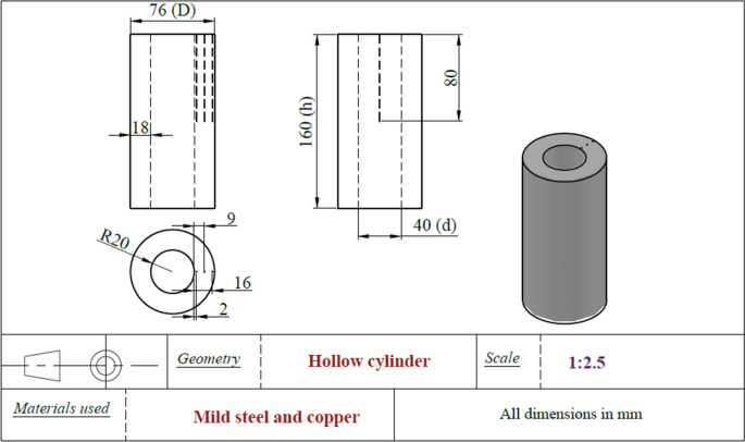

  

  Schematic sketch of the cylindrical mold.

  Figure 4

  

  Schematic sketch of the flat mold.

• b. Experiments involving dipping metallic chill into molten metal.

  In this experimental setup, a small metallic probe was introduced into the melt, and the molten metal was allowed to solidify around the probe to assess the effect of concave and flat contours on casting/chill interfacial heat flux transients (Figure 5). Cylinder and square bar chills were used to obtain concave and flat contours, respectively. The dimensions are selected to maintain a constant (V/A) ratio of the chill and the casting volume and are given in Table 2.

  Figure 5

  

  (a) Schematic representation of dipping of chills in the molten metal, and (b) the corresponding heat flow directions.

  Table 2 Dimensions of Chills Used in the Experiment

Chills were fabricated using mild steel and are instrumented with K-type thermocouples at a depth of 35 mm from the top as shown in Figures 6 and 7, to record the thermal history of the chills. Mild steel chills were also coated with graphite by dip coating to assess the effect of coating on the interfacial heat transfer.

Figure 6

Schematic sketch of the cylindrical chill.

Figure 7

Schematic sketch of the square bar chill.

A semi-automatic table lifter was designed and fabricated in-house. The machine consists of a frame holding an instrumented chill vertically upright and a horizontal table to lift the mold with molten metal (Figure 8a). The table is coupled to a ball screw and nut assembly. A 12 volt DC motor powers ball screw and nut assembly. As the horizontal table lifts up the mold, the chill gets immersed into the melt. Chills are immersed into the molten metal to a height of 60 mm at the rate of 20 mm/s. Chills are positioned stationary to avoid errors in the recorded thermal history. Molds made of mild steel are used, and their dimensions are shown in Figure 8b. The molds are also heated to the melt temperature to prevent solidification of the casting against the mold wall and to ensure heat transfer occurs predominantly at the casting/chill interface.

Figure 8

(a) 12 volt DC motor operated table lifter, (b) Dimensions of the steel mold.

AlSi11Cu3Fe alloy (ADC-12) was used in the present investigation. The chemical composition of aluminum alloy is given in Table 3.

Table 3 Chemical composition of AlSi11Cu3Fe alloy (ADC-12)

The alloy was melted in a resistance-heating furnace to a temperature of 680°C. The melt pouring temperature and the melt in dipping experiments were all maintained at 680°C. Hexachloroethane tablet was added to the melt as a degasser to prevent defects like porosity. After removing the crucible from the furnace, the oxide layer at the top of the melt is skimmed off before pouring. Thermocouples were connected to a computer through a data acquisition system (NI-c-DAQ 9213) (Figure 9). The sampling rate was 0.2 s during temperature data acquisition. The recorded thermal histories and thermophysical properties of the mold/chill were used as input to the inverse heat conduction model to determine the heat flux transients at the casting/mold (chill) interface. The thermophysical properties of copper and mild steel used in the numerical estimation of heat flux transients at the interface are given in Table 4.

Figure 9

Schematic representation of experimental setup. (1), (2), (3), and (4) are the different molds/chills used, (a) K-type thermocouples, (b) connecting wires, (c) data acquisition system, and (d) Laptop computer.

Table 4 Thermophysical Properties of Copper and Mild Steel³⁸

Boundary conditions for estimating interfacial heat flux transients are schematically represented for different mold and chill contours in Figure 10 and 11, respectively. Heat transfer from the casting surface into the mold/chill was estimated by Beck’s nonlinear estimation technique of solving the inverse heat conduction problem. The aim was to compare the effect of casting contour on heat transfer from casting into the mold/chill. TmmFe Inverse solver (Thermet Solutions, Bangalore) was used for this purpose. It is assumed that the heat flow within the mold/chill is one-dimensional (perpendicular to the mold/chill surface in contact with the casting).

Figure 10

Boundary conditions for solving Inverse Heat Conduction Problem in (a) flat and (b) convex mold contour.

Figure 11

Boundary conditions for solving Inverse Heat Conduction Problem in flat and concave chill contours.

The one-dimensional heat conduction equation (Equation 1) is solved using the following boundary and initial conditions.

$$ \frac{\partial }{{\partial {\text{x}}}}\left( {{\text{k}}\frac{{\partial {\text{T}}}}{{\partial {\text{x}}}}} \right) = {\rho C}_{{\text{p}}} \left( {\frac{{\partial {\text{T}}}}{{\partial {\text{t}}}}} \right) $$

(1)

T (L_j, t) = Y (t) (Measured thermocouple temperature at different locations from the mold/chill surface), T (L, t) = B (t) (Thermal boundary condition at the outer surface of the mold/chill), T (L, 0) = T_i (Initial temperature).

where L is the mold/chill thickness.

To determine the unknown heat flux transients (q(t)) at the casting/mold (chill) interface, an error function F(q), expressed as in Equation 2, has to be minimized with respect to q. F(q) represents the sum of squared error between the measured temperature $\left( {{\text{Y}}_{{{\text{n}} + {\text{i}},{\text{j}}}} } \right)$ and the calculated temperature $\left( {{\text{T}}_{{{\text{n}} + {\text{i}},{\text{j}}}} } \right)$ at different thermocouple locations. The time is vectorized as time step numbers. Subscripts ${\text{n}}$ and ${\text{i}}$ correspond to the global time step number and the future time step, respectively. ${\text{m}}$ is the total number of future time steps. j and k correspond to the thermocouple location and total number of thermocouples, respectively.

$$ {\text{F}}\left( {\text{q}} \right) = \left( {\mathop \sum \limits_{{{\text{j}} = 1}}^{{\text{k}}} \mathop \sum \limits_{{{\text{i}} = 1}}^{{\text{m}}} \left( {{\text{ T}}_{{{\text{n}} + {\text{i}},{\text{j}}}} - {\text{Y}}_{{{\text{n}} + {\text{i}},{\text{j}}}} } \right)^{2} } \right) $$

(2)

Initially, for the first global time step number $\left( {{\text{q}}_{{\text{n}}} } \right)$ is arbitrarily assumed (say 100 W/m²). The heat conduction equation is then solved for m future time steps with a constant value of heat flux. An iteration method was employed to estimate ${\text{q}}_{{\text{n}}}$, and the minimization of F(q) led to a correction term for heat flux, as shown in Equation 3. The superscript ${\text{l}}$ indicates the iteration number.

$$ \nabla {\text{q}}_{{\text{n}}}^{{\text{l}}} = \frac{{\mathop \sum \nolimits_{{{\text{j}} = 1}}^{{\text{k}}} \mathop \sum \nolimits_{{{\text{i}} = 1}}^{{\text{m}}} \left( {{\text{Y}}_{{{\text{n}} + {\text{i}},{\text{j}}}} - {\text{T}}_{{{\text{n}} + {\text{i}},{\text{j}}}}^{{{\text{l}} - 1}} } \right)\emptyset_{{{\text{i}},{\text{j}}}}^{{{\text{l}} - 1}} }}{{\mathop \sum \nolimits_{{{\text{j}} = 1}}^{{\text{k}}} \mathop \sum \nolimits_{{{\text{i}} = 1}}^{{\text{m}}} (\emptyset_{{{\text{i}},{\text{j}}}}^{{{\text{l}} - 1}} )^{2} }} $$

(3)

The sensitivity coefficient $\phi_{{{\text{i}},{\text{j}}}}^{{{\text{l}} - 1}}$, defined as the change in calculated temperature (T_n+i,j) when the heat flux ${\text{q}}_{{\text{n}}}$ is increased by a small value $\left( {{\text{q}}_{{\text{n}}}^{{\text{l}}} = {\text{q}}_{{\text{n}}}^{{{\text{l}} - 1}} + {\varepsilon q}_{{\text{n}}}^{{{\text{l}} - 1}} } \right)$, is calculated as shown below.

$$ \emptyset_{{{\text{i}},{\text{j}}}}^{{{\text{l}} - 1}} = \frac{{{\text{T}}_{{{\text{n}} + {\text{i}},{\text{j}}}} ({\text{q}}_{{\text{n}}}^{{{\text{l}} - 1}} \left( {1 + {\upvarepsilon }} \right) - {\text{T}}_{{{\text{n}} + {\text{i}},{\text{j}}}} \left( {{\text{q}}_{{\text{n}}}^{{{\text{l}} - 1}} } \right)}}{{{\varepsilon q}_{{\text{n}}}^{{{\text{l}} - 1}} }} $$

(4)

The correction term is added to the heat flux obtained in the previous iteration, as shown in Equation 5.

$$ {\text{q}}_{{\text{n}}}^{{\text{l}}} = {\text{q}}_{{\text{n}}}^{{{\text{l}} - 1}} + \nabla {\text{q}}_{{\text{n}}}^{{\text{l}}} $$

(5)

The iteration was continued until $\frac{{\nabla {\text{q}}_{{\text{n}}}^{{\text{l}}} }}{{{\text{q}}_{{\text{n}}}^{{{\text{l}} - 1}} }} < 0.005$. The final iterated value of q was used as the initial heat flux for the next global time step.^39,40

Results and Discussion

Effect of Convex and Flat Mold Contour on Interfacial Heat Transfer

Figures 12 and 13 show the thermal history of molds during the solidification of alloy against different mold materials and contours.

Figure 12

Thermal history inside mild steel molds for (a) flat contour, and (b) convex contour during solidification of the alloy.

Figure 13

Thermal history inside copper molds for (a) flat contour, and (b) convex contour during solidification of the alloy.

The thermal history of mild steel molds indicates that after the liquid metal was poured, the location near the interface was heated rapidly to the highest temperature. This can be seen from the recorded thermal history measured by the thermocouple near the interface (TC-1) for mild steel molds. At locations away from the interface, the temperature gradually increases and remains nearly constant after a certain period of time. The temperature profile of TC-1 rises to a peak value when the molten metal makes a conforming contact with the surface of the mold, irrespective of the mold contour. The change in the heating rate of the mold after the peak at TC-1 is because of the non-conforming contact/evolution of air gap at the casting/mold interface caused by the contraction of the solidified skin layer away from the mold surface. The thermocouples located away from the mold surface continue to heat slowly until all the thermocouples instrumented in the mold approach equilibrium.

For mild steel mold with flat contour, a very large difference in temperature of about 131 °C was observed between the thermocouples TC-1 and TC-2 after 5 s from pouring. In contrast, the difference is only 66 °C for the mold with convex contour. For copper molds, the temperature difference between TC-1 and TC-2 at 5 s is 22 °C and 7.5 °C for flat and convex contours, respectively. Thermal plots of the heating chills at 5 s after pouring are shown in Figures 14 and 15.

Figure 14

Thermal plots of flat contoured mold at 5 s after pouring for (a) Mild steel, and (b) Copper.

Figure 15

Thermal plots of convex contoured mold at 5 s after pouring for (a) Mild steel, and (b) Copper.

The thermal plots show the isotherms indicating heat penetration inside the mold. The mild steel mold’s lower thermal conductivity and diffusivity results in a steeper temperature gradient and slower heat conduction from the casting/mold interface to the outer surface. The thermal field images also showed that the heat transfer within the chill is one-dimensional throughout the experiment.

Heat Flux Transients

Figures 16 and 17 show the heat flux transients estimated at the casting/mold interface during solidification of the alloy against copper and mild steel molds with flat and convex mold contours. The estimation of heat flux transients at the casting/mold interface is done by using the boundary conditions shown in Figure 10. At the casting/mold interface, the heat flux shows a maximum shortly after pouring of the liquid metal. Liquid metal first establishes contact with the surface of the mold resulting in a rapid increase in heat flux followed by a peak (q_max). A solidified shell forms, and as the thickness of solidified shell increases with time, the casting skin contracts away from the chill, leading to non-conforming contact at the interface. The decrease in the heat flux after a peak is due to the change of conforming to non-conforming contact at the interface. For mild steel molds, the time of occurrence of peak heat flux is 4.8 s and 3.8 s for flat and convex contours, respectively. The peak heat flux for copper molds occurs early at 3 s and 2.2 s for flat and convex contour, respectively. The estimated peak heat flux transients and the area under the curve for the aluminum alloy solidifying in different molds are listed in Table 5. The area under the curve indicates the total amount of heat extracted per unit area.

Figure 16

Heat flux transients at the casting/mold interface for mild steel molds with flat and convex contour.

Figure 17

Heat flux transients at the casting/mold interface for copper molds with flat and convex contour.

Table 5 Estimated Peak Heat Flux Values and Total Heat Removed for the Molds

Peak heat flux transients were higher for molds with flat contour than convex contour. An increase in peak heat flux of 23 % and 8 % was observed with flat contour compared to convex contour for mild steel and copper molds, respectively. The peak occurs early for copper mold with a flat contour. This is attributed to the high thermal conductivity of copper. The occurrence of peak heat flux is more influenced by the thermal diffusivity of the mold material than its contour. The total energy absorbed by the flat contour was about 17-22% higher than the convex contour for both mold materials. Even though, the (V/A) ratio of casting is constant for both the contour, the (V/A) ratio of the mold with flat contour (4.6 cm) is greater than the (V/A) ratio of the mold with convex contour (2.6 cm) in the experiments carried out. The volumetric heat capacity of mild steel mold calculated for flat contour is 2452 J.K⁻¹, 35 % more than that of the mold with convex contour (1821 J.K⁻¹). The higher the (V/A) ratio of mold higher will be the heat transferred to the mold per unit area. Hence, contrary to the expectation of higher heat flux, the convex interface resulted in a lower flux. The study suggests that to compare the effect of mold contour, the (V/A) ratio of the molds must be the same.

The experimental setup involving dip experiments uses chills with different contours with the same (V/A) ratio. Figure 18 thermal behavior of uncoated and graphite-coated chills dipped into the steel mold during solidification of the alloy. The corresponding variations in heat flux with time are given in Figure 19. The values of peak heat flux of coated and uncoated chills are given in Table 6.

Figure 18

Effect of chill contours on temperature history of (a) bare mild steel chills, and (b) graphite coated mild steel chills, mold material: steel.

Figure 19

Heat flux transients at the casting/chill interface for (a) bare, and (b) graphite-coated mild steel chills dipped into the molten metal; mold material: steel.

Table 6 Estimated Peak Heat Flux Values and Total Heat Removed for the Chills

The thermal history of the chills shows that the chill with flat contour is heated faster than the chill with a concave contour. Higher peak heat flux is recorded for both uncoated chill contours. The peak heat flux in the case of graphite-coated chill is low because of thermal resistance between the outer graphite coating and the inner steel wall. In order to reduce the casting/mold heat transfer, the molds are pre-heated to 650°C before the experiment. This is done primarily to ensure that the heat transfer occurs predominantly at the casting/chill interface rather than the casting/mold interface. For uncoated chills, a 37% increase in the peak heat flux was observed with the flat chill contour compared to concave contour when steel mold is used. A 96 % increase in peak heat flux was observed for chills coated with graphite. Thermal resistance offered by the graphite coating layer of ~96 µm are 2.20 x 10^-4 K/W and 2.80 x 10^-4 K/W for flat and concave surfaces, respectively. Thus, when the chill is heated at a slower rate due to the additional thermal resistance offered by the coating, the effect of chill contour on the peak heat flux becomes more significant. A significant increase in the total energy absorbed by the chill was observed with flat contour than the concave chill contour. The total energy absorbed by the flat and concave contours are 16620 kJ/m² and 8394 kJ/m², respectively, for uncoated chills. For coated chills, the corresponding values are 14339 kJ/m² and 7333 kJ/m², respectively. The flat interface yielded higher heat flux transients in all the experiments compared to concave interface, which is in agreement with the observation reported in the literature.³⁷ As the (V/A) ratio of chill and casting volume is maintained constant, the change in heat flux transients is solely attributed to the contour effect.

It is also important to note that while comparing the effect of contours of different mold materials, the volumetric thermal effusivity (VTE) per unit area of the surface (A) in contact with the casting has to be considered. The volumetric thermal effusivity is defined as (√kρCp)(V). For example, in the present investigation for mild steel molds, the VTE/A of flat mold (549 Ws^1/2m^-1K^-1) was found to be greater than the mold with the convex contour (309 Ws^1/2m^-1K^-1); hence, higher heat flux transients are obtained. The corresponding VTE/A of copper mold were 1715 Ws^1/2m^-1K^-1 and 964 Ws^1/2m^-1K^-1, respectively. The effect of VTE/A on peak heat flux and total heat removed is shown in Figure 20. The argument holds good for chills as well.

Figure 20

Effect of volumetric thermal effusivity per unit area on (a) peak flux and (b) total heat removed.

Conclusions

An experimental setup was designed and fabricated to study the effect of casting contour on interfacial heat flux transients. The heat flux increased rapidly as the liquid metal filled the mold cavity and reached a peak value. The decrease in the heat flux is due to the change of thermal contact condition from conforming to non-conforming at the interface. The effect of three different casting contours on the interfacial heat transfer during the solidification of AlSi11Cu3Fe alloy (ADC-12) was investigated. Based on the results and discussion, the following conclusions are drawn:

• 1. The thermal fields within the mold material estimated using the inverse analysis show that the heat transfer within the mold is one-dimensional throughout the experiment.

• 2. With both square and cylindrical molds representing flat and convex interfaces, heat flux was higher for the flat interface. This was due to the higher mold volume to surface area associated with the square mold.

• 3. For the same (V/A) ratio of the casting, the flat interface resulted in higher heat flux than the convex interface.

• 4. Copper molds resulted in higher heat flux transients than steel molds for all contours.

• 5. Molds with higher volumetric thermal effusivity per unit heat transfer surface area (VTE/A) result in higher heat flux transients. Copper molds with a higher VTE/A ratio yielded higher heat flow rates. Thus, with both copper and steel molds, the flat contour resulted in higher heat flux than convex contour.

• 6. For steel chills with the same (V/A) ratio, the magnitude of the heat flux transients and the heat flow are higher with flat and lower with the concave interface.

• 7. The contour effect becomes more significant for coated chills due to additional thermal resistance.

• 8. To assess the effect of mold contour on heat transfer during solidification, it is essential that (VTE/A) ratio of the mold and the casting volume have to be maintained constant.

References

Z. Chen, Y. Li, F. Zhao, S. Li, J. Zhang, Progress in numerical simulation of casting process. Meas. Control (United Kingdom) 55(5–6), 257–264 (2022). https://doi.org/10.1177/00202940221102656
I. Malik, A.A. Sani, A. Medi, Study on using casting simulation software for design and analysis of riser shapes in a solidifying casting component. J. Phys. Conf. Ser. 1500, 012036 (2020). https://doi.org/10.1088/1742-6596/1500/1/012036
W.D. Griffiths, The heat-transfer coefficient during the unidirectional solidification of an Al-Si alloy casting. Metall. Mater. Trans. B 30, 473–482 (1999). https://doi.org/10.1007/s11663-999-0081-y
K. Narayan Prabhu, W.D. Griffiths, Metal/mould interfacial heat transfer during solidification of cast iron in sand moulds. Int. J. Cast Met. Res. 14(3), 147–155 (2001). https://doi.org/10.1080/13640461.2001.11819433
K. Ho, R.D. Pehlke, Metal-Mold interfacial heat transfer. Metall. Trans. B 16, 585–594 (1985). https://doi.org/10.1007/BF02654857
A.S. Dhodare, P.M. Ravanan, N. Dodiya, A review on interfacial heat transfer coefficient during solidification in casting. Int. J. Eng. Res. Technol. 6(2), 464–467 (2017)
K. Narayan Prabhu, H. Mounesh, K.M. Suresh, A.A. Ashish, Casting/mould interfacial heat transfer during solidification in graphite, steel and graphite lined steel moulds. Int. J. Cast Met. Res. 15(6), 565–571 (2003). https://doi.org/10.1080/13640461.2003.11819542
V.E. Bazhenov, Y.V. Tselovalnik, A.V. Koltygin, V.D. Belov, Investigation of the interfacial heat transfer coefficient at the metal-mold interface during casting of an A356 aluminum alloy and AZ81 magnesium alloy into steel and graphite molds. Int. J. Metal cast. 15, 625–637 (2021). https://doi.org/10.1007/s40962-020-00495-2
M. Asif, M.M. Sadik, Inverse analysis of mould-casting interfacial heat transfer towards improved castings. Mater. Today: Proc. 56, 742–748 (2022). https://doi.org/10.1016/j.matpr.2022.02.248
R. Helenius, O. Lohne, Heat transfer to the die wall during high pressure die casting of two aluminium alloys, part 1. Int. J. Metal cast. 9, 51–59 (2015). https://doi.org/10.1007/BF03355615
A. Zhang, S. Liang, Z. Guo, S. Xiong, Determination of the interfacial heat transfer coefficient at the metal-sand mold interface in low pressure sand casting. Exp. Therm. Fluid Sci. 88, 472–482 (2017). https://doi.org/10.1016/j.expthermflusci.2017.07.002
W. Kasprzak, M. Sahoo, J. Sokolowski, H. Yamagata, H. Kurita, The effect of the melt temperature and the cooling rate on the microstructure of the Al-20% Si alloy used for monolithic engine blocks. Int. J. Metal cast. 3(3), 55–71 (2009). https://doi.org/10.1007/BF03355453
M. Ayabe, T. Nagaoka, K. Shibata, H. Nozute, H. Koyama, K. Ozaki, T. Yanagisawa, Effect of high thermal conductivity die steel in aluminum casting. Int. J. Metal cast. 2, 47–55 (2008). https://doi.org/10.1007/BF03355427
J.I. Cho, C.W. Kim, The relationship between dendrite arm spacing and cooling rate of Al-Si casting alloys in high pressure die casting. Int. J. Metal Cast. 8, 49–55 (2014). https://doi.org/10.1007/BF03355571
H.S. Kim, I.S. Cho, J.S. Shin, S.M. Lee, B.M. Moon, Solidification parameters dependent on interfacial heat transfer coefficient between aluminum casting and copper mold. ISIJ Int. 45(2), 192–198 (2005). https://doi.org/10.2355/isijinternational.45.192
K. Narayan Prabhu, K.M. Suresha, Effect of superheat, mold, and casting materials on the metal/mold interfacial heat transfer during solidification in graphite-lined permanent molds. J. Mater. Eng. Perform. 13(5), 619–626 (2004). https://doi.org/10.1361/10599490420647
M. Kan, Determination of the casting-mold interface heat transfer coefficient for numerically die-casting process depending on different mold temperatures. J. Mech. Sci. Technol. 37(1), 427–433 (2023). https://doi.org/10.1007/s12206-022-1240-1
T. Vossel, N. Wolff, B. Pustal, A. Bührig-Polaczek, Influence of die temperature control on solidification and the casting process. Int. J. Metal cast. 14, 907–925 (2020). https://doi.org/10.1007/s40962-019-00391-4
H. Yavuz, O. Ertugrul, Numerical analysis of the cooling system performance and effectiveness in aluminum low-pressure die casting. Int. J. Metal cast. 15, 216–228 (2021). https://doi.org/10.1007/s40962-020-00446-x
M. Kan, O. Ipek, A numerical and experimental investigation of the thermal behavior of a permanent metal mold with a conventional cooling channel and a new cooling channel design. Int. J. Metal cast. 16, 699–712 (2022). https://doi.org/10.1007/s40962-021-00633-4
Y. Tian, D. Yang, M. Jiang, B. He, Accurate simulation of complex temperature field in counter-pressure casting process using A356 aluminum alloy. Int. J. Metal cast. 15, 259–270 (2021). https://doi.org/10.1007/s40962-020-00456-9
Ö. Boydak, M. Savaş, B. Ekici, A numerical and an experimental investigation of a high-pressure die-casting aluminum alloy. Int. J. Metal cast. 10, 56–69 (2016). https://doi.org/10.1007/s40962-015-0004-4
D. Sui, Z. Cui, R. Wang, S. Hao, Q. Han, Effect of cooling process on porosity in the aluminum alloy automotive wheel during low-pressure die casting. Int. J. Metal cast. 10(1), 32–42 (2016). https://doi.org/10.1007/s40962-015-0008-0
S.A. Hassasi, M. Abbasi, S.J. Hosseinipour, Parametric investigation of squeeze casting process on the microstructure characteristics and mechanical properties of A390 aluminum alloy. Int. J. Metal cast. 14, 69–83 (2020). https://doi.org/10.1007/s40962-019-00325-0
T. Vossel, N. Wolff, B. Pustal, A. Bührig-Polaczek, M. Ahmadein, Heat transfer coefficient determination in a gravity die casting process with local air gap formation and contact pressure using experimental evaluation and numerical simulation. Int. J. Metal cast. 16, 595–612 (2022). https://doi.org/10.1007/s40962-021-00663-y
K.M. Shamil, D.K. Nathan, K.N. Prabhu, Wettability and interfacial heat transfer during solidification of Al–Si Alloy (A413) melt droplets on metallic substrates. Int. J. Metal cast. (2023). https://doi.org/10.1007/s40962-023-00999-7
B. Aksoy, M. Koru, Estimation of casting mold interfacial heat transfer coefficient in pressure die casting process by artificial intelligence methods. Arab. J. Sci. Eng. 45(11), 8969–8980 (2020). https://doi.org/10.1007/s13369-020-04648-7
G. Purushotham, J. Hemanth, Action of chills on microstructure, mechanical properties of chilled ASTM A 494 M grade nickel alloy reinforced with fused SiO2 metal matrix composite. Procedia Mater. Sci. 5, 426–433 (2014). https://doi.org/10.1016/j.mspro.2014.07.285
T.S.P. Kumar, K.N. Prabhu, Heat flux transients at the casting/chill interface during solidification of aluminum base alloys. Metall. Trans. B 22(5), 717–727 (1991). https://doi.org/10.1007/BF02679028
G. Ramesh, K.N. Prabhu, Heat transfer at the casting/chill interface during solidification of commercially pure Zn and Zn base alloy (ZA8). Int. J. Cast Met. Res. 25(3), 160–164 (2012). https://doi.org/10.1179/1743133611Y.0000000026
K. Prabhu, K. Sharath, G. Ramesh, Heat flux transients and casting surface macro-profile during downward solidification of Al-12% Si alloy against chills. Int. J. Metal cast. 5, 63–70 (2011). https://doi.org/10.1007/BF03355523
M.A. Gafur, M.N. Haque, K.N. Prabhu, Effect of chill thickness and superheat on casting/chill interfacial heat transfer during solidification of commercially pure aluminium. J. Mater. Process. Technol. 133(3), 257–265 (2003). https://doi.org/10.1016/S0924-0136(02)00459-4
K.N. Prabhu, J. Campbell, Investigation of casting/chill interfacial heat transfer during solidification of Al-11% Si alloy by inverse modelling and real-time x-ray imaging. Int. J. Cast Met. Res. 12(3), 137–143 (1999). https://doi.org/10.1080/13640461.1999.11819351
J.E. Spinelli, I.L. Ferreira, A. Garcia, Evaluation of heat transfer coefficients during upward and downward transient directional solidification of Al–Si alloys. Struct. Multidiscip. Optim. 31(3), 241–248 (2006). https://doi.org/10.1007/s00158-005-0562-9
I. Rajkumar, N. Rajini, Metal casting modelling software for small scale enterprises to improve efficacy and accuracy. Mater. Today Proc. 46, 7866–7870 (2021). https://doi.org/10.1016/j.matpr.2021.02.542
Z. Chen, Y. Li, F. Zhao, S. Li, J. Zhang, Progress in numerical simulation of casting process. Meas. Control. 55(5–6), 257–264 (2022)
D.R. Poirier, G.H. Geiger, Transport Phenomena in Materials Processing, 1st edn. (Springer, Switzerland, 2016), pp.331–334
M.P. Mughal, H. Fawad, R. Mufti, Parametric thermal analysis of a single molten metal droplet as applied to layered manufacturing. Heat Mass Transf. 42(3), 226–237 (2006). https://doi.org/10.1007/s00231-005-0010-9
K.N. Prabhu, A.A. Ashish, Inverse modeling of heat transfer with application to solidification and quenching. Mater. Manuf. Process. 17(4), 469–481 (2002). https://doi.org/10.1081/AMP-120014230
J.V. Beck, Nonlinear estimation applied to the nonlinear inverse heat conduction problem. Int. J. Heat Mass Transfer. 13, 703–716 (1970). https://doi.org/10.1016/0017-9310(70)90044-X
Acknowledgements
The first author thanks the National Institute of Technology Karnataka for the Ph.D. research fellowship from the Ministry of Education, Government of India.
Author information
Authors and Affiliations
Corresponding author
Additional information
Publisher's Note
Springer Nature remains neutral with regard to jurisdictional claims in published maps and institutional affiliations.
Rights and permissions
Springer Nature or its licensor (e.g. a society or other partner) holds exclusive rights to this article under a publishing agreement with the author(s) or other rightsholder(s); author self-archiving of the accepted manuscript version of this article is solely governed by the terms of such publishing agreement and applicable law.
About this article
Cite this article
Nathan, D.K., Prabhu, K.N. Effect of Mold Contour on Interfacial Heat Transfer During Solidification of AlSi11Cu3Fe Alloy (ADC-12). Inter Metalcast 18, 2133–2149 (2024). https://doi.org/10.1007/s40962-023-01163-x
Received:
Accepted:
Published:
Issue Date:
DOI: https://doi.org/10.1007/s40962-023-01163-x