Bounded generation and commutator width of Chevalley groups: function case

Abstract

We prove that Chevalley groups over polynomial rings $\mathbb {F}_q[t]$ and over Laurent polynomial $\mathbb {F}_q[t,t^{-1}]$ rings, where $\mathbb {F}_q$ is a finite field, are boundedly elementarily generated. Using this we produce explicit bounds of the commutator width of these groups. Under some additional assumptions, we prove similar results for other classes of Chevalley groups over Dedekind rings of arithmetic rings in positive characteristic. As a corollary, we produce explicit estimates for the commutator width of affine Kac–Moody groups defined over finite fields. The paper contains also a broader discussion of the bounded generation problem for groups of Lie type, some applications and a list of unsolved problems in the field.

1 Introduction

In the present paper, we consider Chevalley groups $G=G(\Phi ,R)$ and their elementary subgroups $E(\Phi ,R)$ over various classes of rings, primarily over Dedekind rings of arithmetic type. In some special cases these groups are closely related to various Kac–Moody type groups, and we can derive some non-trivial corollaries in this situation.

Primarily, we are interested in the classical problems of estimating the width of $G(\Phi ,R)$ and $E(\Phi ,R)$ with respect to the following two paradigmatic generating sets:

• The elementary generators $x_{\alpha }(\xi )$, $\alpha \in \Phi$, $\xi \in R$. We say that a group G is boundedly elementarily generated if it has finite width $w_{\textrm{E}}(G)$ with respect to elementary generators.

• Commutators $[x,y]=xyx^{-1}y^{-1}$, where $x,y\in G$. In this case we say that G has finite commutator width $w_{\textrm{C}}(G)$.

(To treat the cases where G is not perfect, we define its commutator width as supremum of the commutator lengths of the elements of the commutator subgroup [G, G]; abusing notation, we still denote it by $w_{\textrm{C}}(G)$ and keep this notation and convention throughout the paper; see Sects. 3.1, 3.2 where the arising subtleties are discussed in some detail.)

In the proofs we work also with other related generating sets, such as elements in the unipotent radicals of various parabolic subgroups, which are closely related but better behaved with respect to stability maps.

For Chevalley groups of rank $\geqslant 2$, bounded generation in terms of elementary generators and bounded generation in terms of commutators are essentially equivalent. Indeed, in this case the Chevalley commutator formula readily implies that every elementary generator of G lying in [G, G] can be presented as a product of a bounded number of commutators. Conversely, a very deep result by Alexei Stepanov and others (see in particular [66, 77], and in final form [76]) implies that given any commutative ring R, every commutator in $E(\Phi ,R)$ is a product of not more than L elementary generators, with the bound $L=L(\Phi )$ depending on $\Phi$ alone. But of course the actual estimates of $w_{\textrm{E}}(G)$ and $w_{\textrm{C}}(G)$ can be very different.

Both problems have attracted considerable attention over the last 40 years or so. Roughly, the situation is as follows. Bounded elementary generation always holds with obvious bounds for 0-dimensional rings and usually fails for rings of dimension $\geqslant 2$. But for 1-dimensional rings it is problematic.

Thus, from the existence of arbitrary long division chains in Euclidean algorithm it follows that and are not boundedly elementarily generated. But this could be attributed to the exceptional behaviour of rank 1 groups. Much more surprisingly, Wilberd van der Kallen [83] established that bounded generation fails even for , a group of Lie rank 2 over a Euclidean ring!

An emblematic example of 1-dimensional rings are Dedekind rings of arithmetic type , for which bounded elementary generation of $G(\Phi ,R)$ is intrinsically related to the positive solution of the congruence subgroup problem in that group. This connection was first noted by Vladimir Platonov and Andrei Rapinchuk, see [56, 60, 61].

For the number case the situation is well understood, even for rank 1 groups. After the initial breakthrough by Douglas Carter and Gordon Keller [9, 10], later expanded by Oleg Tavgen [78] and many others, we now know bounded generation with excellent bounds depending on the type of $\Phi$ and the class number of R for all Chevalley groups of rank $\geqslant 2$. Apart from the rings , $|S|=1$, with finite multiplicative group, similar results are even available for , see a detailed survey in Sect. 3.

However, the function case turned out to be much more recalcitrant, and is not solved up to now, apart from some important but isolated results, such as the works by Clifford Queen [59] and Bogdan Nica [51], which treat the group over some arithmetic function rings with infinite multiplicative groups, and the groups , $n\geqslant 3$, respectively.¹

Here we expand these results to all Chevalley groups, obtaining explicit bounds. The first major new result of the present paper establishes bounded elementary generation for all Chevalley groups of rank at least 2 over the most classical, and in a sense the most difficult example, polynomial rings ${\mathbb {F}}_{q}[t]$ with coefficients in finite fields.²

Theorem A

Let $G(\Phi ,R)$ be a simply connected Chevalley group of type $\Phi$, over $R={\mathbb {F}}_{q}[t]$. Then the width of $G(\Phi ,R)$ with respect to elementary generators is bounded by a constant not depending on q.

The proof of this result constitutes about half of the paper. Some bound in the bounded generation for all Chevalley groups can be easily derived from the case of rank two systems by a version of the usual Tavgen’s trick [78, Theorem 1], described in [68, 89].

• For $\textsc {A}_2$ bounded generation of is precisely the main result of Nica [51].

• A large part of the present paper is the analysis of the most difficult case of , which is the Chevalley group of type $\textsc {C}_2$. Again, we take the proof in Tavgen’s paper [78, Section 4], as a prototype. But there is a substantial difference, since now we have to verify some arithmetic properties that are well known in the number case, but for which we could not find any reference in the function case.

• Luckily, we do not have to imitate Tavgen’s proof [78, Section 5], for the remaining case of the Chevalley group of type $\textsc {G}_2$. Instead of a difficult direct calculation, we show that this case can be derived from the case of $\textsc {A}_2$ by the usual stability arguments.

For there is a realistic bound of the width in elementary generators, in terms of stability conditions, taking into account the fact that for Dedekind rings . The aforementioned proof of Theorem A gives us an occasion to return to the stability arguments for all Chevalley groups, and obtain bounds which are substantially better than the ones that could be obtained via Tavgen’s trick.

Alternatively, Theorem A can be restated in the following equivalent form. The difference is that in this case the computations of many authors, subsumed and expanded by Andrei Smolensky [67], allow one to produce very reasonable bounds, usually at most 6, 7 or 8 commutators.

Theorem B

Let $G(\Phi ,R)$ be a simply connected Chevalley group of type $\Phi$, over $R={\mathbb {F}}_{q}[t]$. Then $G(\Phi ,R)$ is of finite commutator width.

Remark 1.1

The commutator width of a Chevalley group of type $\Phi$ depends on the lattice $\mathscr {P}$ determining it. For example, $w_{\textrm{C}}({{\,\textrm{PSL}\,}}(2,{\mathbb {Q}}))=1$ while (the matrix $-I$ is not representable as a single commutator and is a product of two commutators, see [79]). So, if the lattice is not stated explicitly, under $w_{\textrm{C}}(G(\Phi ,R))$ we always mean maximum, i.e., the commutator width of the simply connected group.

See Sect. 3.2 for the discussion of subtleties arising in the cases where G is not perfect.

In fact, for applications to Kac–Moody groups we do not need the full force of Theorem A. We only need a similar result for the equally classical but much easier example of Laurent polynomial rings ${\mathbb {F}}_{q}[t,t^{-1}]$ with coefficients in finite fields.

For Chevalley groups over such rings bounded generation can be derived from Theorem A. Yet, the bounds thus obtained will not be the best possible ones. However, the multiplicative group of the ring $R={\mathbb {F}}_{q}[t,t^{-1}]$ is infinite. This means that alternatively bounded generation can be derived—with much better bounds!—from the result by Clifford Queen [59]. Let us state the most spectacular finiteness result in terms of unitriangular factors obtained along this route.

Theorem C

Let be the ring of S-integers of K, a function field of one variable over ${\mathbb {F}}_q$ with S containing at least two places. Assume that at least one of the following holds:

• either at least one of these places has degree one, or

• the class number of R, as a Dedekind domain, is prime to $q-1$.

Then any simply connected Chevalley group $G=G(\Phi ,R)$ admits the following decompositions:

$$\begin{aligned} G=UU^-UU^-U=U^-UU^-UU^-. \end{aligned}$$

Such a sharp bound was quite unexpected for us. In particular, Chevalley groups over such arithmetic rings have the same commutator width as Chevalley groups over rings of stable rank 1, see [67].

In particular, we can now give the same bounds for affine Kac–Moody groups.

Theorem D

The commutator width of an affine elementary untwisted Kac–Moody group ${\widetilde{E}}_{\textrm{sc}}(A,{\mathbb {F}}_q)$ over a finite field ${\mathbb {F}}_q$ is $\leqslant L'$, where

• for $\Phi =\textsc {F}_4$ and $\Phi =\textsc {A}_l$, $l=2k+1$, $k=0,1,\dots$;

• for $\Phi =\textsc {A}_l$, $l=2k$, $k=1,2,\dots$, $\Phi =\textsc {B}_l, \textsc {C}_l, \textsc {D}_l$, for $l\geqslant 3$ or $\Phi =\textsc {E}_7, \textsc {E}_8$, or, finally, $\Phi =\textsc {C}_2, \textsc {G}_2$ under the additional assumption that 1 is the sum of two units in R (which is automatically the case provided $q\ne 2$);

• for $\Phi =\textsc {E}_6$.

The paper is organised as follows. In Sect. 2 we recall the necessary notation and preliminaries and in Sect. 3 provide background and historical survey. The next four sections constitute the technical core of the paper. Namely, in Sect. 4 we sketch the scheme of the proof of Theorem A, of which Theorem B is an immediate corollary, and reduce its proof to the rank 2 groups. This reduction is a variation of Tavgen’s rank reduction trick, a further slight improvement of the rank reduction results in [68, 89]. In Sect. 5 we revisit surjective stability for $K_1$ modeled on Chevalley groups, with explicit bounds, and, in particular, reduce the case of the group $\textrm{G}_2(R)$ to the known case of . In Sect. 6 we prove Theorem A for the group , which is the most exciting case of all, and requires rather difficult algebraic and arithmetic considerations. Section 7 contains an alternative argument based on reducing to rank 3 groups and separate consideration of the types $\textsc {B}_3$ and $\textsc {C}_3$. Incidentally, this gives estimates with better constants. After that, in Sect. 8 we develop an alternative approach to bounded elementary generation, based on Queen’s result, that gives sharper bounds for some classes of rings R with infinite multiplicative groups, including Laurent polynomial rings, thus proving Theorem C. The next section is devoted to applications. In Sect. 9.1 we discuss applications to Kac–Moody groups over finite fields and prove Theorem D, and in Sect. 9.2 we obtain some applications of bounded generation in model theory. Finally, in Sect. 10 we present some relevant concluding remarks and open problems.

2 Notation and preliminaries

In this section we briefly recall the notation that will be used throughout the paper. For more details on Chevalley groups over rings see [87, 88], where one can find many further references.

2.1 Chevalley groups

Let $\Phi$ be a reduced irreducible root system of rank $\geqslant 2$, and $W=W(\Phi )$ be its Weyl group. Choose an order on $\Phi$ and let and $\Pi =\{\alpha _1,\ldots ,\alpha _l\}$ be the corresponding sets of positive, negative and fundamental roots, respectively. Further, we consider a lattice intermediate between the root lattice and the weight lattice . Finally, let R be a commutative ring with 1, with the multiplicative group $R^*$.

These data determine the Chevalley group , of type over R. It is usually constructed as the group of R-points of the Chevalley–Demazure group scheme of type . In the case the group G is called simply connected and is denoted by $G_{{\text {sc}}}(\Phi ,R)$. In another extreme case the group G is called adjoint and is denoted by $G_{{\text {ad}}}(\Phi ,R)$. Many results do not depend on the lattice and hold for all groups of a given type $\Phi$. In all such cases, or when is determined by the context, we omit any reference to in the notation and denote by $G(\Phi ,R)$ any Chevalley group of type $\Phi$ over R. Usually, we assume that $G(\Phi ,R)$ is simply connected.

In what follows, we also fix a split maximal torus $T=T(\Phi ,R)$ in $G=G(\Phi ,R)$ and identify $\Phi$ with $\Phi (G,T)$. This choice uniquely determines the unipotent root subgroups, $X_{\alpha }$, $\alpha \in \Phi$, in G, elementary with respect to T. As usual, we fix maps $x_{\alpha }:R\mapsto X_{\alpha }$, so that $X_{\alpha }=\{x_{\alpha }(\xi )\,{|}\,\xi \in R\}$, and require that these parametrisations are interrelated by the Chevalley commutator formula with integer coefficients, see [13, 75]. The above unipotent elements $x_{\alpha }(\xi )$, where $\alpha \in \Phi$, $\xi \in R$, elementary with respect to $T(\Phi ,R)$, are also called [elementary] unipotent root elements or, for short, simply root unipotents.

Further,

$$\begin{aligned} E(\Phi ,R)=\langle x_\alpha (\xi ),\, \alpha \in \Phi ,\, \xi \in R\rangle \end{aligned}$$

denotes the absolute elementary subgroup of $G(\Phi ,R)$, spanned by all elementary root unipotents, or, what is the same, by all [elementary] root subgroups $X_{\alpha }$, $\alpha \in \Phi$.

Since we are interested in the bounded generation, we also consider the subset $E^L(\Phi ,R)$, consisting of products of $\leqslant L$ root unipotents. Since $E^L(\Phi ,R)$ contains all generators of $E(\Phi ,R)$, it is not a subgroup of $E(\Phi ,R)$, unless $E^L(\Phi ,R)=E(\Phi ,R)$.

2.2 Root elements

Further, let $\alpha \in \Phi$ and $\varepsilon \in R^{*}$. As usual, we set

The elements $h_{\alpha }(\varepsilon )$ are called semisimple root elements.

By definition, $h_{\alpha }(\varepsilon )$ is a product of six elementary unipotents—well, actually if you look inside, five of them. However, it is classically known that $h_{\alpha }(\varepsilon )$ is a product of four elementary unipotents³. To somewhat improve some of the ulterior bounds we need a still more precise form of this classical observation, asserting that the first/last of these four factors can be chosen either lower, or upper, with an arbitrary invertible parameter. After that the remaining three factors are uniquely determined.

The following fact is obvious, but we could not find an explicit reference.

Lemma 2.1

Let R be any commutative ring. Then for any $\varepsilon ,\eta \in R^*$ the matrix $h_{\alpha }(\varepsilon )$ can be represented as the product of the form

Proof

Verify one of these formulae by a direct calculation in , then transpose, invert and transpose-invert it.$\square$

Corollary 2.2

Let R be any commutative ring. Then for any $\varepsilon ,\lambda \in R^*$ the matrix $h_{\alpha }(\varepsilon )$ can be transformed to $h_{\alpha }(\lambda )$ by four elementary moves.

Proof

By Lemma 2.1, $h_\alpha (\varepsilon \lambda ^{-1})=h_\alpha (\varepsilon ) (h_\alpha (\lambda ))^{-1}$ can be transformed to 1 by four elementary moves, whence the statement.$\square$

Next, let $N=N(\Phi ,R)$ be the algebraic normaliser of the torus $T=T(\Phi ,R)$, i.e. the subgroup, generated by $T=T(\Phi ,R)$ and all elements $w_{\alpha }(1)$, $\alpha \in \Phi$. The factor-group N/T is canonically isomorphic to the Weyl group W, and for each $w\in W$ we fix its preimage $n_{w}\in N$. Clearly, such a preimage can be taken in $E(\Phi ,R)$. Indeed, for a root reflection $w_{\alpha }$ one can take $w_{\alpha }(1)\in E(\Phi ,R)$ as its preimage, any element w of the Weyl group can be expressed as a product of root reflections.

In particular, we get the following classical result, which is crucial in reduction to smaller ranks.

Lemma 2.3

The elementary Chevalley group $E(\Phi ,R)$ is generated by unipotent root elements $x_{\alpha }(\xi )$, $\alpha \in \pm \Pi$, $\xi \in R$, corresponding to the fundamental and negative fundamental roots.

Further, let $B=B(\Phi ,R)$ and be a pair of opposite Borel subgroups containing $T=T(\Phi ,R)$, standard with respect to the given order. Recall that B and $B^-$ are semidirect products $B=T{\rightthreetimes }\hspace{1.111pt}U$ and , of the torus T and their unipotent radicals

Here, as usual, for a subset X of a group G one denotes by $\langle X\rangle$ the subgroup in G generated by X. Semidirect product decomposition of B amounts to saying that $B=TU=UT$, and at that and $T\cap U=1$. Similar facts hold with B and U replaced by $B^-$ and $U^-$. Sometimes, to speak of both subgroups U and $U^-$ simultaneously, we denote $U=U(\Phi ,R)$ by .

2.3 Levi decomposition

The main role in the reduction to smaller ranks is played by Levi decomposition for elementary parabolic subgroups. In general, one can associate a subgroup $E(S)=E(S,R)$ to any closed set $S\subseteq \Phi$. Recall that a subset S of $\Phi$ is called closed, if for any two roots $\alpha ,\beta \in S$ the fact that $\alpha +\beta \in \Phi$, implies that already $\alpha +\beta \in S$. Now, we define $E(S)=E(S,R)$ as the subgroup generated by all elementary root unipotent subgroups $X_{\alpha }$, $\alpha \in S$:

$$\begin{aligned} E(S,R)=\langle x_{\alpha }(\xi ),\, \alpha \in S, \, \xi \in R\rangle . \end{aligned}$$

In this notation, U and $U^{-}$ coincide with and , respectively. The groups E(S, R) are particularly important in the case where S is a special (= unipotent) set of roots; in other words, where $S\cap (-S)=\varnothing$. In this case E(S, R) coincides with the product of root subgroups $X_{\alpha }$, $\alpha \in S$, in some/any fixed order.

Let again $S\subseteq \Phi$ be a closed set of roots. Then S can be decomposed into a disjoint union of its reductive (= symmetric) part $S^{\textrm{r}}$, consisting of those $\alpha \in S$, for which $-\alpha \in S$, and its unipotent part $S^{\textrm{u}}$, consisting of those $\alpha \in S$, for which $-\alpha \not \in S$. The set $S^{\textrm{r}}$ is a closed root subsystem, whereas the set $S^{\textrm{u}}$ is special. Moreover, $S^{\textrm{u}}$ is an ideal of S, in other words, if $\alpha \in S$, $\beta \in S^{\textrm{u}}$ and $\alpha +\beta \in \Phi$, then $\alpha +\beta \in S^{\textrm{u}}$. Levi decomposition asserts that the group E(S, R) decomposes into semidirect product of its Levi subgroup and its unipotent radical .

Especially important is the case of elementary subgroups corresponding to the maximal parabolic subschemes. Denote by $m_k(\alpha )$ the coefficient of $\alpha _k$ in the expansion of $\alpha$ with respect to the fundamental roots:

Now, fix an $r=1,\ldots ,l$—in fact, in the reduction to smaller rank it suffices to employ only terminal parabolic subgroups, even only the ones corresponding to the first and the last fundamental roots, $r=1,l$. Denote by

$$\begin{aligned} S=S_r=\{\alpha \in \Phi : m_r(\alpha )\geqslant 0\} \end{aligned}$$

the r-th standard parabolic subset in $\Phi$. As usual, the reductive part $\Delta =\Delta _r$ and the special part $\Sigma =\Sigma _r$ of the set $S=S_r$ are defined as

$$\begin{aligned} \Delta =\{\alpha \in \Phi : m_r(\alpha ) = 0\},\quad \Sigma =\{\alpha \in \Phi : m_r(\alpha ) > 0\}. \end{aligned}$$

The opposite parabolic subset and its special part are defined similarly

Obviously, the reductive part $S^-_r$ equals $\Delta$.

Denote by $P_r$ the elementary [maximal] parabolic subgroup of the elementary group $E(\Phi ,R)$. By definition,

$$\begin{aligned} P_r=E(S_r,R)=\langle x_\alpha (\xi ),\, \alpha \in S_r, \, \xi \in R \rangle . \end{aligned}$$

Now Levi decomposition asserts that the group $P_r$ can be represented as the semidirect product

of the elementary Levi subgroup $L_r=E(\Delta ,R)$ and the unipotent radical $U_r=E(\Sigma ,R)$. Recall that

$$\begin{aligned} L_r=E(\Delta ,R)=\langle x_\alpha (\xi ),\, \alpha \in \Delta , \, \xi \in R \rangle , \end{aligned}$$

whereas

$$\begin{aligned} U_r=E(\Sigma ,R)= \langle x_\alpha (\xi ),\, \alpha \in \Sigma ,\, \xi \in R\rangle . \end{aligned}$$

A similar decomposition holds for the opposite parabolic subgroup $P_r^-$, whereby the Levi subgroup is the same as for $P_r$, but the unipotent radical $U_r$ is replaced by the opposite unipotent radical $U_r^-=E(-\Sigma ,R)$.

As a matter of fact, we use Levi decomposition in the following form. It will be convenient to slightly change the notation and write $U(\Sigma ,R)=E(\Sigma ,R)$ and $U^-(\Sigma ,R)=E(-\Sigma ,R)$.

Lemma 2.4

The group $\langle U^{\sigma }(\Delta ,R),U^\rho (\Sigma ,R)\rangle$, where $\sigma ,\rho =\pm 1$, is the semidirect product of its normal subgroup $U^\rho (\Sigma ,R)$ and the complementary subgroup $U^{\sigma }(\Delta ,R)$.

In other words, it is asserted here that the subgroups $U^{\pm }(\Delta ,R)$ normalise each of the groups $U^{\pm }(\Sigma ,R)$, so that, in particular, one has the following four equalities for products:

and, furthermore, the following four obvious equalities for intersections hold:

$$\begin{aligned} U^{\pm }(\Delta ,R)\cap U^{\pm }(\Sigma ,R)=1. \end{aligned}$$

In particular, one has the following decompositions:

3 Bounded generation. State of art

To put the results of the present paper in context, here we briefly recall what is known concerning the finite elementary width and the finite commutator width of Chevalley groups over rings. This will give us an occasion to explain some basic ideas behind our proof.

3.1 Length and width

Let G be a group and X be a set of its generators. Usually one considers symmetric sets, for which .

• The length $l_X(g)$ of an element $g\in G$ with respect to X is the minimal k such that g can be expressed as the product $g=x_1\ldots x_k$, $x_i\in X$.

• The width $w_X(G)$ of G with respect to X is the supremum of $l_X(g)$ over all $g\in G$.

We say that a group G has bounded generation with respect to X if the width $w_X(G)$ is finite.⁴ In the case when $w_X(G)=\infty$, one says that G does not have bounded word length with respect to X.

The problem of calculating or estimating $w_X(G)$ has attracted a lot of attention, especially when G is one of the classical-like groups over skew-fields.

There are hundreds of papers which address this problem in the case when G is a classical group such as or or its large subgroup, whereas X is a natural set of its generators.

• Classically, over fields and other small-dimensional rings one would think of elementary transvections, all transvections, or Eichler–Siegel–Dickson (ESD)-transvections, reflections, pseudo-reflections, or other small-dimensional transformations.

• Other common choice would be a class of matrices determined by their eigenvalues such as the set of all involutions, a non-central conjugacy class, or the set of all commutators.

• More exotic choices include matrices distinct from the identity matrix in one column, symmetric matrices, etc.

In many classical cases exact values or at least sharp estimates of $w_X(G)$ are available. Sometimes there are even more precise results, explicitly calculating the length of individual elements in terms of certain geometric invariants such as, e.g., the dimension of its residual space, or the like.

More generally, oftentimes one considers any subset $X\subseteq G$ and looks at the width $w_X(\langle X\rangle )$. For instance, one calls the width of the commutator subgroup [G, G] with respect to the set of all commutators the commutator width of G itself, regardless of whether the group G is perfect. This is a prototypical example of what is called the word length problems, when one tries to calculate or estimate the width of the verbal subgroup of G with respect to a word w with respect to the set of values of w in G.

3.2 Elementary width and commutator width

In the present paper we focus on the much less studied case, where $G=G(\Phi ,R)$ is a Chevalley group or its elementary subgroup $E(\Phi ,R)$ over a commutative ring R, and on the closely related case of Kac–Moody groups. In this setting exact calculations of $w_X(G)$ with respect to most of the generating sets are usually beyond reach.

In the present paper we are primarily interested in the two following candidates for the generating set X for $E(\Phi ,R)$:

• The set of elementary root unipotents

  $$\begin{aligned} \Omega =\{x_{\alpha }(\xi )\,{|}\, \alpha \in \Phi ,\xi \in R\} \end{aligned}$$

  relative to the choice of a split maximal torus T.

• The set of commutators

  $$\begin{aligned} C=\bigl \{[x,y]=xyx^{-1}y^{-1}\,{|}\, x\in G(\Phi ,R),\, y\in E(\Phi ,R)\bigr \}. \end{aligned}$$

It is a classical theorem due to Suslin, Kopeiko and Taddei that for one indeed has $C\subseteq E(\Phi ,R)$.

The width $w_{\Omega }(E(\Phi ,R))$ is usually denoted $w_{\textrm{E}}(G(\Phi ,R))$ and is called the elementary width of $G(\Phi ,R)$. Clearly, $w_{\textrm{E}}(G(\Phi ,R))$ is the smallest L such that$E(\Phi ,R)=E^L(\Phi ,R)$.

Similarly, the width $w_{\textrm{C}}(E(\Phi ,R))$ is oftentimes called the commutator width of $G(\Phi ,R)$ itself.

Remark 3.1

Notice the subtleties related to the necessity to distinguish the Chevalley group $G(\Phi ,R)$ itself, its commutator, the elementary subgroup $E(\Phi ,R)$, etc. In the arithmetic situation they usually all coincide in ranks $\geqslant 2$, even in the relative case, this is precisely the [almost] positive solution of the congruence subgroup problem. But for the group (and occasionally for some groups of rank 2) one will have to impose additional restrictions.

Anyway, in the arithmetic case for simply connected groups of rank at least two it follows from [46] that $G_{{\text {sc}}}(\Phi ,R)=E_{{\text {sc}}}(\Phi ,R)$. This means that the above set C equals the set of all commutators in $G_{{\text {sc}}}(\Phi ,R)$. That said, one sees that Theorem B is indeed equivalent to Theorem A.

One has to mention the exceptional cases where G is not perfect. For groups of rank at least 2, this happens if and only if R has ${\mathbb {F}}_2$ among its residue fields and $\Phi$ is of type $\mathrm C_2$ or $\mathrm G_2$. In the case where R is a field, this was first noticed by Robert Steinberg [74]. For more general rings, this was proved by Michael Stein [71, Corollary 4.4]. Note that no additional exceptions arise even for reductive groups, see [44].

Inside the proofs we have to consider some other related generating sets, such as, for instance:

• the set of all unitriangular elements

  $$\begin{aligned} U(\Phi ,R)\cup U^-(\Phi ,R); \quad \text {or} \end{aligned}$$

• the set of all root unipotents

  $$\begin{aligned} \Omega ^G=\bigl \{x_{\alpha }(\xi )^g \,{|}\ \alpha \in \Phi ,\,\xi \in R,\, g\in G(\Phi ,R)\bigr \}, \end{aligned}$$

which are better behaved with respect to reduction to smaller ranks.

3.3 The case of 0-dimensional rings

Finiteness of the elementary width is a very rare and extremely significant phenomenon which has repercussions everywhere in the structure theory of the group. It is obvious, and classically known that Chevalley groups over fields and semi-local rings have finite elementary width. In fact, the groups over 0-dimensional rings rejoice short factorisations such as Bruhat decomposition or Gauß decomposition. Such factorisations are essentially tantamount to bounded elementary generation with very sharp bounds.

In fact, Bruhat decomposition immediately implies that over a field the elementary width of $G(\Phi ,K)$ does not exceed $2N+4l$ (here and below $N=|\Phi ^+|$, ). It immediately follows that the commutator width of $G(\Phi ,K)$ is also finite.

But determining the precise value of the commutator width turned out to be a very challenging problem—for finite fields it was the famous Ore conjecture. Without trying to follow the whole tortuous path, we just mention the two definitive contributions. For fields containing $\geqslant 8$ elements Erich Ellers and Nikolai Gordeev [EG] using Gauß decomposition with prescribed semi-simple part have proven that $w_{\textrm{C}}(G_{{\text {ad}}}(\Phi ,R))=1$, while $w_{\textrm{C}}(G_{{\text {sc}}}(\Phi ,R))\leqslant 2$. This was then extended to the groups over small fields ${\mathbb {F}}_{q}$, $q=2, 3, 4, 5, 7$, by Martin Liebeck, Eamonn O’Brien, Aner Shalev, and Pham Huu Tiep [40, 41], using explicit information about their maximal subgroups and very delicate character estimates.

Similarly, Gauß decomposition which holds over arbitrary semi-local rings—or even over rings of stable rank 1, see [68]⁵ in particular—implies that the elementary width of $G(\Phi ,R)$ does not exceed $3N+4l$. Actually, [89] gives another estimate in terms of unitriangular decomposition, 4N, which is usually better for groups of very small ranks, say, up to 4 or 5. What seems to not have been noted in the literature, is that the LUP-decomposition of Chevalley groups over local rings provides the same upper bound on their width as for fields, $2N+4l$.

As above, bounded elementary generation implies finite commutator width. However, providing sharp bounds for this width turned out to be a difficult problem. Skipping a detailed description of the early work by Keith Dennis, Leonid Vaserstein, You Hong, and others, pertaining to the classical groups [3, 23, 24, 86], we just mention a recent paper by Andrei Smolensky [67], where such an estimate is obtained for all Chevalley groups. The commutator width $w_{\textrm{C}}(E(\Phi ,R))$ does not exceed 3 for $\Phi =\textsc {A}_l$ and $\textsc {F}_4$, does not exceed 4 for all other types, except maybe for $\textsc {E}_6$, and does not exceed 5 for $G(\textsc {E}_6,R)$. [We strongly believe that the commutator width does not exceed 4 also for $\textsc {E}_6$, but we were discouraged by the extent of calculations necessary to improve the bound in this remaining case.]

Note that so far there are no examples of matrices from , , ($n\geqslant 3$), not representable as a single commutator.

3.4 Counter-examples

The groups of rank 1 only occasionally can have finite elementary width, or finite commutator width, for that matter. Over a Euclidean ring R elementary expressions in correspond to continued fractions.

In fact, the existence of arbitrarily long division chains in $\mathbb {Z}$ and in K[t] implies that the groups and cannot be boundedly generated. The most classical example are the Fibonacci matrices

$$\begin{aligned} \begin{pmatrix} F_{m+1}&{}F_m\\ F_m&{}F_{m-1} \end{pmatrix} \end{aligned}$$

which for even m require precisely m elementary factors.

Remark 3.2

For an odd m a similar matrix looks as

$$\begin{aligned} \begin{pmatrix} F_{m}&{}F_{m+1}\\ F_{m-1}&{}F_{m} \end{pmatrix}, \end{aligned}$$

which strongly suggests that while considering the width problems in it might be more expedient to switch to Cohn’s generators

$$\begin{aligned} \begin{pmatrix} x&{}1\\ 1&{}0 \end{pmatrix}. \end{aligned}$$

Of course, the same holds for , where instead of two consecutive Fibonacci numbers one should take two sufficiently generic polynomials of two consecutive degrees m and $m-1$, placing the one of the higher degree into the NW or NE corner, depending on the parity of m. Many such similar examples were constructed by Paul Cohn [16] and others starting with the mid-1960s.

What came as a shock, though, was that the elementary width of rank $\geqslant 2$ groups over a Euclidean ring can be infinite too. Indeed, using methods of higher algebraic K-theory Wilberd van der Kallen [83] has proven that has infinite elementary width. Later Igor Erovenko came up with a somewhat more elementary proof [26]. On the other hand, soon thereafter Dennis and Vaserstein [24] noticed that does not even have finite commutator width.

3.5 Dedekind rings of arithmetic type, groups of rank $\geqslant 2$

For rings of dimension $\geqslant 2$ one cannot in general expect bounded generation. An extremely interesting borderline case are 1-dimensional rings, especially the classical example of the Dedekind rings of arithmetic type. Below, K is a global field, i.e. a finite extension of $\mathbb {Q}$ in characteristic 0, or a finite extension of ${\mathbb F}_{\!q}(t)$, $q=p^m$, in positive characteristic p. Further, S is a finite set of valuations of K, containing all Archimedean ones in the number case, and .

The number case is well understood. The initial breakthrough was due to David Carter and Gordon Keller who have proven that , $n\geqslant 3$, is boundedly elementary generated and gave explicit bounds on in terms of n and the discriminant⁶ of K, see [9]. The proof in this paper is essentially an effectivisation of the usual verification of the familiar properties of Mennicke symbols.

Actually, their published proof is based on explicit rank reduction in terms of the stable rank, see below. It remains to verify bounded generation of . One of the key calculations in that paper, Lemma 1, can be described as follows. Let be a matrix with the first row (a, b). Then $A^m$ can be transformed to a matrix in with the first row by a sequence of not more than 16 elementary transformations in —sic!

However, Carter and Keller mention that their original approach was based on model theory. To elucidate the connection, recall that van der Kallen [83] observed that the obstruction to bounded elementary generation of the group $E(\Phi ,R)$ is the quotient $E(\Phi ,R)^{\infty }/E(\Phi ,R^{\infty })$ (countably many copies). This establishes connection with ultraproducts and non-standard models. Namely, it can be interpreted as the equivalence of the bounded generation of $E(\Phi ,R)$ and the [almost] positive solution of the congruence subgroup problem for $G(\Phi ,{}^*R)$ for non-standard models ${}^*R$ of R.

Carter and Keller came up with such a proof for the group , initially for $n\geqslant 3$, see [11]. Dave Witte Morris [49] gave an exposition of this proof in a somewhat more traditional logical language (first-order properties, compactness theorem, etc.). Unfortunately, this proof is not much easier than a direct algebraic proof⁷ and it gives no bound whatsoever on the elementary width.

In [10] Carter and Keller have given a separate elementary proof specifically for the [easier] case of , $n\geqslant 3$, in terms of direct matrix manipulations, mimicking the verification of the properties of Mennicke symbols (but without explicitly mentioning the work of Mennicke and/or of Bass–Milnor–Serre [7]). In particular, they have proven that the elementary width of does not exceed 48,⁸ later this bound was reduced by Nica [51] to 37.

Soon thereafter, Oleg Tavgen invented a different, purely elementary approach to rank reduction, which allowed him to reduce the proof of bounded generation for all Chevalley groups to groups of rank 2. After that he succeeded in settling the cases of rank 2 groups, and the Chevalley group of type $\textsc {G}_2$ (and, in fact, also twisted Chevalley groups of rank 2) by direct matrix calculations. These important advances sum up to his main result, the bounded elementary generation of Chevalley groups of rank $\geqslant 2$ over arithmetic Dedekind rings in the number case.

3.6 Dedekind rings of arithmetic type, groups of rank 1

There is a critical difference in behaviour of , depending on whether $|S|=1$, in which case $R^*$ is finite, and $|S|\geqslant 2$, when $R^*$ is infinite. As we know, for the case $|S|=1$ the answer to the question on bounded elementary generation is negative, so in the rest of the subsection we assume that $R^*$ is infinite.

Again in the number case the situation is well understood. Elementary generation of is closely related to generalisations of Euclidean algorithm. Important early inroads in this direction were suggested [apparently independently!] by Timothy O’Meara [54], who simultaneously considered the number case and the function case, and by Paul Cohn [16], who proposed vast [non-commutative] generalisations.

About a decade later, George Cooke and Peter Weinberger [19] systematically studied the length of division chains [17, 18] in the number case. For the case, where $R^*$ is infinite, their main results implied that modulo some form of the Generalised Riemann Hypothesis (GRH), any matrix in is a product of $\leqslant 9$ elementary transvections.

The results of Hendrik Lenstra on the Generalised Artin Conjecture [39]—again conditional on GRH—imply that whenever S contains at least one real valuation, the bound here can be reduced to $\leqslant 7$. Observe that the best possible bound here is⁹$\leqslant 5$. However, Cooke and Weinberger proposed an example of a matrix over a totally imaginary ring R of degree 4 which cannot be expressed as a product of less than six elementary matrices.

It has taken quite some time to get rid of the dependence on the GRH and to improve bounds here. Modulo the GRH, Bruce Jordan and Yevgeny Zaytman [35] have slightly remodelled the Cooke–Weinberger argument and improved the bound to five elementary transvections if K is not totally imaginary, to six elementary transvections when S contains at least one non-Archimedean place, and to seven elementary transvections for the integers of a totally imaginary field.

One of the first unconditional results was obtained by Bernhard Liehl [42], but he imposed some additional restrictions on the number field K, and his proof does not give good bounds. Almost simultaneously Carter and Keller, jointly with Eugene Paige, came up with the first general logical proof [12], somewhat refashioned in [49]. But, as we already mentioned, this proof gives no bounds whatsoever. About a decade later Loukanidis and Murty [43, 50] proposed an unconditional analytic argument, but it only works provided S is sufficiently large, say .

Some 10 years ago Maxim Vsemirnov and Sury [90] considered the key example of , obtaining the bound $\leqslant 5$ unconditionally. This was a key inroad to the first complete unconditional solution of the general case with a good bound, in the work of Alexander Morgan, Andrei Rapinchuk and Sury [48]. The bound they gave is $\leqslant 9$, but for the case when S contains at least one real or non-Archimedean valuation¹⁰ it was almost immediately improved [with the same ideas] to $\leqslant 8$ by Jordan and Zaytman [35].

3.7 Reduction to smaller ranks

Let us explain, what do the width bounds obtained for ranks 1 or 2 imply for higher ranks.

There are two basic ways to reduce the problem of bounded generation for a Chevalley groups to similar problems for groups of smaller ranks. We will start with Tavgen’s reduction theorem, which came later historically, but is both more elementary and more general, than the reduction based on stability conditions. On the other hand, explicit factorisations resulting from stability conditions are not always available, but when they are, they give sharper bounds.

To present Tavgen’s idea in its simplest form, let us consider not the width in elementary generators, but a coarser problem of determining the width of $G(\Phi ,R)$ in terms of the elements belonging to the unipotent subgroups U and $U^-$. As far as we know, this problem was first systematically considered by Dennis and Vaserstein in the context of the closely related problem of estimating the commutator width for , see [23, 24]. In other words, we are interested in finding the smallest m such that

where the last factor equals U or $U^-$ depending on whether m is odd or even.

Essentially, Tavgen observed that if there are root subsystems $\Psi _1,\ldots ,\Psi _t\subseteq \Phi$ which contain all fundamental roots, and such that each of the Chevalley groups $G(\Psi _1,R), \ldots , G(\Psi _t,R)$ admits a similar decomposition with m factors, then $G(\Phi ,R)$ itself admits such a decomposition with m factors. In this [and in fact slightly more general] form this reduction is described in [68, 89]. Modulo the Levi decomposition of parabolic subgroups and the Chevalley commutator formula it is undergraduate group theory, see the next section for precise statements, somewhat broader discussion, and a proof.

Since every element of U is a product of not more than $N=|\Phi ^+|$ elementary generators, Tavgen’s theorem suffices to give plausible bounds for the elementary width of large rank groups in terms of the elementary widths of their rank 1 or rank 2 subgroups. However, these bounds tend to be somewhat exaggerated.

Actually, for small dimensional rings there is a more precise form of reduction in terms of the stability conditions. For such a reduction in terms of the usual stable rank was first proposed by Hyman Bass in 1964, and then improved by Vaserstein, Dennis, Kolster, and others. Namely, for the usual proof of the surjective stability for ${\text {SK}}_1$ grants the following decomposition:

It follows that if has the elementary width $\leqslant s$, then has the elementary width $\leqslant s+4n$ — and in fact , if you look inside the proof.

For Dedekind rings this bound was slightly improved by Carter and Keller [9], who noticed that one can do slightly better by observing that . This means that for $n\geqslant 2$ one needs just one addition instead of two, to get a shorter unimodular row. This gives for the elementary width of the estimate $s+\frac{3}{2}n^2-{\frac{1}{2}}n-5$, where s is the elementary width of $\textrm{SL}\hspace{0.55542pt}(2,R)$.

Surjective stability of ${\text {K}}_1$ in terms of various stability conditions—the usual stable rank , the absolute stable rank , or the like—is known for all relevant embeddings of other Chevalley groups. For the usual stability embeddings of classical groups of the same type, it is indeed classical, starting with the work of Anthony Bak and Leonid Vaserstein. For cross-type and exceptional emdeddings such similar results were established by Michael Stein and Eugene Plotkin, see in particular [57, 58, 72, 73]. However, at least in the exceptional cases it was not stated in the form of such precise decompositions as above.

As a result, the explicit bounds for other groups—let alone their improvements for Dedekind rings—were never mentioned in the available literature. Even in the number case Tavgen only states finiteness, without providing any specific bound. In Sect. 5 below, as part of the proof of Theorem A, we return to this problem, and procure such explicit bounds.

Let us mention yet another extremely pregnant generalisation, bounded reduction. In fact, even below the usual stability conditions and even in the absence of the bounded generation for $G(\Psi ,R)$, it makes sense to speak of the number of elementary generators necessary to reduce an element g of $G(\Phi ,R)$ to an element of $G(\Psi ,R)$, for a subsystem $\Psi \subseteq \Phi$.

One such prominent example are polynomial rings $R[t_1,\ldots ,R_m]$, where bounded reduction holds starting with a rank depending on R alone, not on the number of indeterminates. For the case of this is essentially an effectivisation of Suslin’s solution of the ${\text {K}}_1$-analogue of Serre’s problem, explicit bounds were obtained in the remarkable paper by Leonid Vaserstein [84], which unfortunately remained unpublished. For other split classical groups such bounds were recently obtained by Pavel Gvozdevsky [32].

3.8 The function case

In the function case, until now much less was known concerning the bounded generation of Chevalley groups. On the one hand, an analogue of Riemann’s Hypothesis was known in this case for quite some time. On the other hand, in the positive characteristic additional arithmetic difficulties occur, that have no obvious counterparts in characteristic 0. They reflect in particular in the structure of arithmetic subgroups in the function case. For instance, it is well known that the group $\textrm{SL}\hspace{0.55542pt}(2,K[t])$ is not even finitely generated, whereas the groups and are finitely generated but not finitely presented.

Until very recently the only published result was that by Clifford Queen [59]. We discuss this and related work in much more detail in Sect. 8. Queen’s main result implies that under some additional assumptions on R—which hold, for instance, for Laurent polynomial rings ${\mathbb {F}}_{q}[t,t^{-1}]$ with coefficients in a finite field—the elementary width of the group is $\leqslant 5$. As we know, this implies, in particular, bounded elementary generation of all Chevalley groups $G(\Phi ,R)$.

The case of the groups over the usual polynomial ring long remained open. Only in 2018 has Bogdan Nica established the bounded elementary generation of , $n\geqslant 3$. Part of the problem is that in characteristic $p>0$ bounded elementary generation is not the same as bounded generation in terms of cyclic subgroups. For instance, the groups do not have bounded generation in this abstract sense, see [1].

This is exactly where we jump in. As already stated in the introduction, in the present paper we prove bounded elementary generation for all Chevalley groups of rank $\geqslant 2$ over the usual polynomial rings and—with better bounds—for Chevalley groups of rank $\geqslant 1$ over a class of function rings with infinite multiplicative group, including the Laurent polynomial rings .

3.9 Further prospects

The historical description is already rather long, we cannot mention many further aspects. A systematic survey should include at least:

• Partial positive results, such as bounded expressions of elementary conjugates and commutators in terms of elementary generators—decomposition of unipotents, Stepanov’s universal localisation, and the like.

• Connection with the prestability kernel, bounded generation of in terms of Vaserstein prestability generators, [85], etc.

• Connection of the bounded generation with the congruence subgroup problem, Kazhdan’s property (T), finite presentation, super-rigidity, etc.

• Implications for the bounded generation by cyclic/abelian subgroups, including actions, etc.

• Extension of known bounds for word width (such as in [6]) to the function case.

We intend to return to [some of] these subjects in an expected sequel to the present paper.

4 Outline of the proof of Theorem A and reduction to rank 2

In this section we sketch the main ideas of the proof and implement the rank reduction. Together with the result by Nica [51], this already suffices to establish Theorem A for simply laced types and type ${\textsc {F}}_4$.

4.1 Outline of the proof

The proofs of bounded generation for the rings of integers of an algebraic number field, see [2, 9, 10, 78], deploy similar ideas. Let

$$\begin{aligned} A=\left( \begin{array}{cc} a&{}b \\ c&{}d \\ \end{array}\right) \end{aligned}$$

be a matrix from nested either in or in . Observe that in the second case there are two natural embeddings of , on short roots and on long roots, and that is a major aspect of the quest. We also provide an approach based on the reduction to Chevalley groups of rank 3. This approach has some advantages and makes use of embeddings of the Chevalley group of type $G(\textsc {A}_2,R)$ into either $G(\textsc {C}_3,R)$ or $G(\textsc {B}_3,R)$. The Chevalley groups of type $\textsc {G}_2$ are to be treated separately anyway, but they do not occur in the analysis of higher rank cases.

The goal is to reduce A to the identity matrix by elementary transformations in G in such a way that the number of elementary factors does not depend on A. The guideline of the proof can be summarised as follows:

• Eventually, one has to transform A to a matrix with an invertible entry by a bounded number of elementary transformations.

• One way to do that is to use a version of Little Fermat’s Theorem. So we need some entry of A in an appropriate power.

• Hence, we need to produce an elementary descendant B of A with some entry, say the first one, to be $a^k$, where k is an appropriate power. This is achieved by Lemmas 1 in [9, 10, 2, Lemma 2], [78, Proposition 3].

• The proof follows from the miraculous fact that the matrix

  $$\begin{aligned} A^k=\left( \begin{array}{cc} a&{}b \\ c&{}d \\ \end{array}\right) ^k \end{aligned}$$

  coincides modulo elementary matrices with the matrix

  $$\begin{aligned} B=\left( \begin{array}{cc} a^k&{}b\\ *&{}* \\ \end{array}\right) . \end{aligned}$$

• This miracle is none other than the multiplicative property of Mennicke symbols, so this is not a surprise at all modulo a tricky proof of this property (see [45, 47], etc).

• It remains to use a combination of analytic tools such as Dirichlet’s theorem on primes in arithmetic progressions and, if needed, reciprocity laws to obtain by elementary transformations a matrix of the form

  $$\begin{aligned} B=\left( \begin{array}{cc} a^k&{}p\\ q&{}* \\ \end{array}\right) \end{aligned}$$

  where the pair satisfies $a^k-1=ps$ for some s.

Note that Nica [51] modified the proof using the so-called “swindling lemma”. We shall discuss this trick in more detail in Sect. 6. Actually, “swindling” is merely a weaker version of the multiplicativity of Mennicke symbols. However, the advantage is that this weaker form is cheaper in terms of the number of elementary moves, and here we generalise this approach to the symplectic case as well.

Remark 4.1

One of the points of the present work is that, unlike the proofs based on model theory, here we get efficient realistic estimates for the number of elementary factors, with bounds that depend on $\Phi$ alone. In some cases, like for the bounded reduction to smaller rank, our bounds are [very close to] the best possible ones. For small ranks, there might be still some gap between the counter-examples and the estimates we obtain, but our upper bounds are still reasonably close to the theoretically best possible ones. The lower bounds in such similar problems are usually quite difficult to obtain, anyway.

4.2 Tavgen’s reduction theorem

Here we reproduce with minor variations the elementary reduction procedure due to Tavgen, in the form mentioned in [68, 89]. This procedure suffices to reduce Theorem A for groups of rank $\geqslant 3$ to the groups and . It of course works also for reduction to and ${{\,\textrm{SO}\,}}(7,R)$ used in Sect. 7. Moreover, the bounds it gives are quite reasonable, though clearly not the best possible ones. In Sect. 5 we work out the stable reduction, based on the fact the stable rank of Dedekind rings equals 1.5. This approach gives much better bounds for reduction, sometimes the sharp ones, and for exceptional groups it is new even in the number case.

Tavgen’s approach works more smoothly for unitriangular factorisations, in other words, for expressions of elementary subgroup $E(\Phi ,R)$ as a product of subgroups $U(\Phi ,R)$ and $U^-(\Phi ,R)$,

Later on in [68] it was applied to triangular factorisations, where also the toral factor is admitted.¹¹

The leading idea of Tavgen’s proof is very general and beautiful, and works in many other related situations. It relies on the fact that for systems of rank $\geqslant 2$ every fundamental root falls into the subsystem of smaller rank obtained by dropping either the first or the last fundamental root. However, as was pointed out by the referee of [68], the argument applies without any modification in a much more general setting. Namely, it suffices to assume that the required decomposition holds for some subsystems $\Delta =\Delta _1,\ldots ,\Delta _t$, whose union contains all fundamental roots of $\Phi$. These subsystems do not have to be terminal, or even irreducible, for that matter!

Theorem 4.2

Let $\Phi$ be a reduced irreducible root system of rank $l\geqslant 2$, and R be a commutative ring. Further, let $\Delta =\Delta _1,\ldots ,\Delta _t$ be some subsystems of $\Phi$, whose union contains all fundamental roots of $\Phi$. Suppose that for all $\Delta =\Delta _1,\ldots ,\Delta _l$, the elementary Chevalley group $E(\Delta ,R)$ admits a unitriangular factorisation

of length L. Then the elementary Chevalley group $E(\Phi ,R)$ itself admits unitriangular factorisation

of the same length L.

Let us reproduce the details of the argument. By definition,

is a subset in $E(\Phi ,R)$. Usually, the easiest way to prove that a subset $Y\subseteq G$ coincides with the whole group G consists in the following

Lemma 4.3

Assume that $Y\subseteq G$, $Y\ne \varnothing$, and let $X\subseteq G$ be a symmetric generating set. If $XY\subseteq Y$, then $Y=G$.

Now, we are all set to finish the proof of Theorem 4.2.

Proof

By Lemma 2.3, the group $E(\Phi ,R)$ is generated by the fundamental root elements

$$\begin{aligned} X=\{x_{\alpha }(\xi )\,{|}\, \alpha \in \pm \Pi ,\, \xi \in R\}. \end{aligned}$$

Thus, by Lemma 4.3 is suffices to prove that $XY\subseteq Y$.

Fix a fundamental root unipotent $x_{\alpha }(\xi )$. Since , the root $\alpha$ belongs to at least one of the subsystems $\Delta =\Delta _r$, where $r=1,\ldots ,t$. Set $\Sigma =\Sigma _r$ and express $U^{\pm }(\Phi ,R)$ in the form

Using Lemma 2.4, we see that

Since $\alpha \in \Delta$, one has $x_{\alpha }(\xi )\in E(\Delta ,R)$, so that the inclusion $x_{\alpha }(\xi )Y\subseteq Y$ immediately follows from the assumption.$\square$

4.3 Proof of Theorem A for simply laced systems and in the case of $\textsc {F}_4$

In [68] the authors commented that they do not see immediate applications of the more general form of Tavgen’s reduction theorem, as stated above. Here, we notice that it is in fact surprisingly strong, since it allows one to pass from some smaller rank subsystems to the whole system, without looking at any other subsystems, including those of intermediate ranks! Indeed, it may happen that for those other subsystems bounded generation holds with some larger bound, or bluntly fails.

Of course, the easiest case is when the group itself has bounded elementary generation.

Corollary 4.4

Let any element of be a product of  $\leqslant L$ elementaries. Then any simply connected Chevalley group $G=G(\Phi ,R)$ admits unitriangular factorisation

$$\begin{aligned} G=UU^-U\cdots U^{\pm } \end{aligned}$$

of length L.

However, this is very seldom the case, so one should start looking at larger rank subsystems. Recall that in the $\textsc {A}_2$ case Theorem A was proven by Nica [51]. His main new result can be stated as follows.

Proposition 4.5

Any element of   is a product of $\leqslant 41$ elementary transvections.

We are not contending for the best possible bounds in terms of unitriangular matrices at this stage, since later we improve the bounds anyway. Interestingly, the main arithmetic ingredient of his proof is the Kornblum–Artin functional version of Dirichlet’s theorem on primes in arithmetic progressions. In Sect. 6 below we shall see how it works in the parallel example of .

Now, together with Theorem 4.2 this result by Nica implies Theorem A for the two following cases:

• Chevalley groups of simply laced type $\Phi$ of rank $\geqslant 2$. Indeed, in this case $\Pi$ is covered by the fundamental copies of $\textsc {A}_2$ spanned by all pairs of adjacent fundamental roots.

• Chevalley group of type $\textsc {F}_4$. Indeed, in this case $\Pi$ is covered by two fundamental copies of $\textsc {A}_2$ — the long one $\textsc {A}_2$, spanned by the two fundamental long roots, and the short one $\widetilde{\textsc {A}}_2$, spanned by the two fundamental short roots.

Observe that in the second case it is neither assumed, nor does it follow that the group is boundedly generated! Even more amazingly, the same applies to the subgroups of types $\textsc {B}_3$ and $\textsc {C}_3$.

However, for root systems of types $\textsc {B}_l$ and $\textsc {C}_l$ there are short/long roots that cannot be embedded into any irreducible rank 2 subsystem other than $\textsc {C}_2$. Thus, to be able to apply Theorem 4.2 we have to explicitly dismantle elements of into elementary factors. This is exactly what is achieved in Sect. 6.

However, since we are interested in actual bounds, before treating this case, we have to recall an alternative approach to rank reduction, based on stability conditions. In the next section we recall the stability conditions themselves and illustrate how they work for Chevalley groups of type $\textsc {G}_2$. Later, in Sects. 5 and 6 we produce similar arguments for groups of types $\textsc {C}_2,\textsc {C}_3$, and $\textsc {B}_3$.

5 Proof of Theorem A in the case of $\textsc {G}_2$

The purpose of this section is two-fold. As a first objective, here we provide the proof of Theorem A for the Chevalley group of type $\textsc {G}_2$. This is done by virtue of surjective stability for the embedding $\textsc {A}_2\longrightarrow \textsc {G}_2$. Using this opportunity, we revisit stability for Dedekind rings also for other embeddings, and obtain accurate bounds for reduction in this case. For exceptional groups such explicit bounds are new even in the number case.

5.1 Stability conditions

Traditionally, stability results are stated in terms of stability conditions. The first such condition, stable rank, was introduced by Hyman Bass back in 1964. However, surjective stability results for $\mathrm K_1$ for embeddings other than the simplest stability embeddings

usually require stronger stability conditions, such as the absolute stable rank, etc.

Modulo some small additive constants, all these ranks are bounded by the Krull dimension or even the Jacobson dimension of the ring R. On the other hand, arithmetic rings, such as Dedekind rings and their kin, usually satisfy even stronger stability conditions than the ones that would follow from their dimension. Here we very briefly recall some of these conditions, limiting ourselves only to those that are actually used in the sequel.

A row is called unimodular if its components $a_1,\ldots ,a_n$ generate R as a right ideal,

$$\begin{aligned} a_1R+\cdots +a_nR=R, \end{aligned}$$

or, what is the same, if there exist $b_1,\ldots ,b_n\in R$ such that

$$\begin{aligned} a_1b_1+\cdots +a_nb_n=1. \end{aligned}$$

A row of length $n+1$ is called stable if there exist $b_1,\ldots ,b_n\in R$ such that the ideal generated by

$$\begin{aligned} a_1+a_{n+1}b_1,\; a_2+a_{n+1}b_2, \; \ldots , \;a_n+a_{n+1}b_n \end{aligned}$$

coincides with the ideal generated by $a_1,\ldots ,a_{n+1}$.

The stable rank of the ring R is the smallest n such that every unimodular row $(a_1,\ldots ,a_{n+1})$ of length $n+1$ is stable. In other words, there exist $b_1,\ldots ,b_n\in R$ such that the row

$$\begin{aligned} (a_1+a_{n+1}b_1,a_2+a_{n+1}b_2,\ldots ,a_n+a_{n+1}b_n) \end{aligned}$$

of length n is unimodular. If no such n exists, one writes .

Bass himself denoted stability of unimodular rows of length $n+1$ by ${{\,\textrm{SR}\,}}_{n+1}(R)$. It is easy to see that condition ${{\,\textrm{SR}\,}}_m(R)$ implies condition ${{\,\textrm{SR}\,}}_n(R)$ for all $n\geqslant m$, so that the stable rank is defined correctly: if , then every unimodular row of length n is stable. Clearly, this means that when one can iterate the process of shortening a unimodular row and eventually reduce any unimodular row to a unimodular row of length .

For representations other than the vector representations of $\textrm{SL}\hspace{0.55542pt}_n$ and , the stock of available elementary transformations is limited, so that one has to work with pieces of unimodular rows, that are not themselves unimodular. However, stability of all non-unimodular rows is an exceedingly restrictive condition — though Dedekind rings satisfy precisely something of the sort!

The most familiar variation of stable rank, that works for other classical groups, is the absolute stable rank. For commutative rings this condition was introduced by David Estes and Jack Ohm [29], whereas Michael Stein [73] discovered its relevance in the study of orthogonal groups and exceptional groups.

For a row $(a_1,\ldots ,a_{n})\in {}^{n}R$ let us denote by $J(a_1,\ldots ,a_{n})$ the intersection of the maximal ideals of the ring R containing $a_1,\ldots ,a_{n}$. In particular, a row is unimodular if and only if $J(a_1,\ldots ,a_{n})=R$.

One says that a commutative ring R satisfies condition ${{\,\textrm{ASR}\,}}_{n+1}$ if for any row $(a_1,\ldots ,a_{n+1})$ of length $n+1$ there exist $b_1,\ldots b_n\in R$ such that

$$\begin{aligned} J(a_1+a_{n+1}b_1,\ldots ,a_n+a_{n+1}b_n)= J(a_1,\ldots ,a_{n+1}). \end{aligned}$$

It is obvious that condition ${{\,\textrm{ASR}\,}}_m(R)$ implies condition ${{\,\textrm{ASR}\,}}_n(R)$ for all $n\geqslant m$. The absolute stable rank of the ring R is the smallest natural n for which condition ${{\,\textrm{ASR}\,}}_{n+1}(R)$ holds. Clearly, .

The classical theorem of Estes and Ohm [29] asserts that for commutative rings one has

a similar estimate for follows from a classical theorem of Bass. Thus, in particular, any Dedekind ring satisfies ${{\,\textrm{ASR}\,}}_3(R)$ — and, as we recall below, a much stronger condition.

5.2 Surjective stability for $\textrm{K}_1$ and bounded reduction.

Recall that the $\mathrm K_1$-functor modelled on a Chevalley group $G(\Phi ,R)$ is defined as

$$\begin{aligned} \mathrm K_1(\Phi ,R)=G(\Phi ,R)/E(\Phi ,R). \end{aligned}$$

For [irreducible] root systems of rank $\geqslant 2$ the elementary subgroup $E(\Phi ,R)$ is a normal subgroup of $G(\Phi ,R)$, so that in this case $\textrm{K}_1(\Phi ,R)$ is a group.

Now, by the homomorphism theorem every embedding of root systems $\Delta \subset \Phi$ gives rise to the stability map

$$\begin{aligned} \nu =\nu _{\Delta \rightarrow \Phi }:\mathrm K_1(\Phi ,\Delta )\longrightarrow \mathrm K_1(\Phi ,R), \end{aligned}$$

and one of the archetypical classical problems of the algebraic $\mathrm K$-theory, whose study was initiated by Hyman Bass in the early 1960s, is to find conditions under which this map is surjective or injective.

Clearly, surjective stability for the embedding $\Delta \subset \Phi$ amounts to the equality

In other words, any matrix $g\in G(\Phi ,R)$ can be expressed as a product of a matrix from $G(\Delta ,R)$ and elementary unipotents.

However, in the stable range, that is when is large with respect to , one can use the above stability conditions and establish rather more. In this setup, all customary proofs of surjective stability afford not just elementary reduction to smaller rank, but bounded elementary reduction. In other words, they establish an equality of the type

for some constant L depending on the dimension of the ring R and the embedding $\Delta \subset \Phi$. This means that we have bounded reduction: any matrix $g\in G(\Phi ,R)$ can be expressed as a product of a matrix from $G(\Delta ,R)$ and not more than L elementary unipotents, where L does not depend on g.

When $\Delta$ is the reductive part of a parabolic subset S of $\Phi$, the actual value of L is estimated in terms of the order of the unipotent part $\Sigma$ of S. Thus, as we have already mentioned in Sect. 4, for the embedding $\textsc {A}_{n-1}\subset \textsc {A}_n$ the original Bass’s proof furnishes the following classical decomposition

which implies that in this case L is at most 4n. Actually, since one needs only additions to shorten a unimodular row, this bound immediately reduces to .

However, for all other embeddings, apart from $\textsc {C}_{n-1}\subset \textsc {C}_n$, and especially for exceptional groups and for root subsystems that are not reductive parts of parabolic subsets, it is not that immediate. Even in the classical cases, not to mention the exceptional ones, the exact number of elementary unipotents used in the reduction was not explicitly tracked.

Indeed, the existing proofs of surjective stability do not bother about explicit bounds. At the moment, one could invoke a previously known stability result with the same or weaker stability condition, one would do that, without actually reproducing the reduction procedure, or worrying for the shortest elementary expressions. For anyone familiar with the proofs of surjective stability in, say [31, 57, 58, 73], it is clear that they afford bounded reduction with some L. Note that these bounds are valid in the case of any base ring of Krull dimension 1 and hence for any Dedeking ring. But any such bounds are not explicit there, and one should go over all proofs in these papers once again even to produce some bounds (not the best possible ones!).

Additional features of the exceptional cases are that—with the sole exception of $\textsc {G}_2$—their minimal representations are too large for manual matrix computations, and even in these representations the elementary unipotents are significantly more complicated. Thus, instead of matrices one should use some tools from representation theory, as do [31, 57, 58, 73]. It would take quite a few pages to describe these tools, and adjust them to our needs. To establish Theorem A with some [reasonable] bound, we do not need that. Actually, we intend to return to this issue in the sequel to this paper, and come up with sharp bounds. In the next section we limit ourselves with the proof specifically for the long root embeddings $\textsc {A}_1\subset \textsc {A}_2\subset \textsc {G}_2$.

5.3 Proof of Theorem A for $\textsc {G}_2$

In his pathbreaking paper [73] Michael Stein proves, in particular, that under the absolute stable range condition ${{\,\textrm{ASR}\,}}_3(R)$ one has

[long root embeddings], this is his Theorem 4.1.m. Below, we go through the proof of that theorem, to come up with an actual bound.

Theorem 5.1

Under the assumption ${{\,\textrm{ASR}\,}}_3(R)$ one has

Clearly, this result together with the main theorem of [51] immediately implies the claim of Theorem A for the case of $\textsc {G}_2$. Indeed, $\textrm{SL}\hspace{0.55542pt}(3,R)$ is boundedly elementary generated, and since Dedekind rings have dimension $\leqslant 1$ and thus satisfy condition ${{\,\textrm{ASR}\,}}_3$, it follows from the above result that

$$\begin{aligned} w_{\textrm{E}}(G(\textsc {G}_2,R))\leqslant w_{\textrm{E}}(G(\textsc {A}_2,R))+24. \end{aligned}$$

Proof

Our proof closely follows that in [73], pages 102–104, and we essentially preserve the notation thereof. Let $\alpha _1,\alpha _2$ be the fundamental roots of $\textsc {G}_2$, with $\alpha _2$ long. Further, consider the short roots

$$\begin{aligned} \alpha =-\alpha _1,\quad \beta =2\alpha _1+\alpha _2,\quad \gamma ={}-\alpha _1-\alpha _2, \end{aligned}$$

which clearly sum to zero, $\alpha +\beta +\gamma =0$.

Consider the 7-dimensional short root representation of $G(\textsc {G}_2,R)$, with the highest weight $\mu =\beta$, its weights are the short roots $\pm \alpha ,\pm \beta ,\pm \gamma$ and 0. Order the weights by height, $\mu =\beta ,-\gamma ,-\alpha ,0,\alpha ,\gamma ,-\beta$.

As usual, the entries of matrices $g\in G(\textsc {G}_2,R)$ are indexed by pairs of weights, $g=(g_{\lambda ,\mu })$, where $\lambda ,\mu =\beta ,\ldots ,-\beta$.

Initially, we concentrate on the first column $g_{*\beta }$ of this matrix, which is the image of the highest weight vector under the action of g. For typographical reasons, we denote this column by

$$\begin{aligned} (x_\beta ,x_{-\gamma },x_{-\alpha },x_0,x_\alpha ,x_\gamma ,x_{-\beta }). \end{aligned}$$

It is our intention to reduce this column to the form $(1,*,*,*,*,*,*)$ by elementary unipotents.

This can be done as follows. Not to proliferate indices in this and further stability calculations, we will not rename [as mathematicians would do], but reset [as is typical in programming] our variables g and x, still denoting them by the same letters after each successive transformation.

In order to make the action of elementary unipotents visible, below we present the weight diagram of the 7-dimensional short root representation of $G(\textsc {G}_2,R)$:

As usual, the action of the elementary unipotent $x_\gamma (t)$ on the first column $g_{*\beta }$ can be viewed by looking for pairs of weights on the weight diagram connected by the root $\gamma$.

• Using condition ${{\,\textrm{SR}\,}}_3(R)$, we can find $a_1,a_2\in R$ such that the shorter column

  $$\begin{aligned} (x_\beta +a_1x_0,x_{-\gamma },x_{-\alpha }+a_2x_0,\_, x_\alpha ,x_\gamma ,x_{-\beta }), \end{aligned}$$

  where the blank indicates the position of the component $x_0$ that we drop, is unimodular. Reset g to —this requires two elementary operations. After this step we may assume that $(x_\beta ,x_{-\gamma },x_{-\alpha },x_\alpha ,x_\gamma ,x_{-\beta })$ is unimodular.

• Observe that every elementary long root unipotent $x_{\delta }(\xi )$ adds one of the components $x_{\beta },x_{\alpha },x_{\gamma }$ to another one of them, acts in the opposite direction on the components $x_{-\beta },x_{-\alpha },x_{-\gamma }$, and fixes $x_0$. This corresponds to the decomposition of the 7-dimensional representation of $G(\textsc {G}_2,R)$ into two 3-dimensional and one 1-dimensional invariant subspaces, when restricted to $G(\textsc {A}_2,R)$.

Thus, we consider the ideal I generated by the components $x_{\beta },x_{\alpha },x_{\gamma }$. As we just observed, this ideal is not changed by the action of any element of $E(\textsc {A}_2,R)$. However, under the condition ${{\,\textrm{SR}\,}}_3(R/I)$ transitivity of the action $\textrm{SL}\hspace{0.55542pt}(3,R)$ in the 3-dimensional vector representation is well known from the work of Bass. For this we need two additions to shorten a unimodular column over R/I of length 3 to two positions, then two additions to get 1 in the third position, and, finally, two additions to clear the components in the remaining two positions. This is six elementary operations altogether.

This means that further multiplying g by six factors of the form $x_{\pm (\beta -\alpha )}(*)$ and $x_{\pm (\beta -\gamma )}(*)$ we obtain a column of height 6

$$\begin{aligned} (x_\beta +a_1x_0,x_{-\gamma },x_{-\alpha }+a_2x_0,\_, x_\alpha ,x_\gamma ,x_{-\beta }), \end{aligned}$$

subject to the extra condition that

$$\begin{aligned} x_{-\beta }\equiv 1\pmod {I},\qquad x_{-\alpha },x_{-\gamma }\equiv 0\pmod {I}. \end{aligned}$$

In other words, already the following column of height 4

$$\begin{aligned} (x_\beta ,\_,\_,\_,x_\alpha ,x_\gamma ,x_{-\beta }). \end{aligned}$$

is unimodular.

So far, we only invoked the usual stable rank condition ${{\,\textrm{SR}\,}}_3$. Next, the tricky part comes, which requires the use of ${{\,\textrm{ASR}\,}}_3$.

• Using condition ${{\,\textrm{ASR}\,}}_3(R)$ we can find $b_1,b_2\in R$ such that the ideal J generated by $x_{\alpha }+b_1x_{\beta },x_{\gamma }+b_2x_{\beta }$ is contained in the same maximal ideals that the [a priori larger] ideal I generated by $x_\beta ,x_\alpha ,x_\gamma$. This means that resetting g to —that is further two elementary operations—we may assume that the following column of height 3

  $$\begin{aligned} (\_,\_,\_,\_,x_\alpha ,x_\gamma ,x_{-\beta }) \end{aligned}$$

  is unimodular.

• Now, using condition ${{\,\textrm{SR}\,}}_3(R)$ once more we can find $c_1,c_2\in R$ such that the following column of height 2

  $$\begin{aligned} (\_,\_,\_,\_,x_\alpha +c_1x_{-\beta },x_\gamma +c_2x_{-\beta },\_) \end{aligned}$$

  is unimodular. As usual, we reset g to —that is two more elementary operations.

• After the previous step we may assume that

  $$\begin{aligned} (\_,\_,\_,\_,x_\alpha ,x_\gamma ,\_) \end{aligned}$$

  is unimodular, and we are done. It remains to express

  $$\begin{aligned} 1-x_{\beta }=d_1x_{\alpha }+d_2x_{\gamma }, \end{aligned}$$

  and to reset g to —that is two more elementary operations—to achieve our intermediate goal $x_{\beta }=1$.

• Up to now we have used 14 elementary operations in $E(\textsc {G}_2,R)$. On the other hand, a matrix g with 1 in the diagonal position corresponding to the highest weight can be readily reduced to smaller rank, in our case,

  

This is exactly the celebrated Chevalley–Matsumoto decomposition theorem, see, for instance [46, 73, 87] (the same argument was used in [78]). But , which consumes $\leqslant 10$ more elementary unipotents, not more 24 elementary factors altogether, as claimed.$\square$

We are in possession of similar reduction results, with pretty sharp bounds, also for all other exceptional cases. But calculations with columns of height 26, 27, 56 and 248 are quite a bit more involved. In the present paper we limit ourselves with some explicit bounds, resulting from Tavgen’s approach. We intend to come up with much sharper bounds in the sequel to this paper.

5.4 Improvements for Dedekind rings

As is well known, for Dedekind rings the constants in the reduction can be slightly improved. This is based on the well-known property that the ideals I in Dedekind rings are not just 2-generated, but rather 1.5-generated. In other words, one of the generators can be an arbitrary non-zero element of I.

More precisely, let be an ideal of a Dedekind ring R. Then for any $a\in I$, $a\ne 0$, there exists $b\in I$ such that $aR+bR=I$. This translates into the following stability condition, weaker than , but strictly stronger than .

Lemma 5.2

Let R be a Dedekind ring, and be its ideal. Then for any three elements $a,b,c\in R$ generating I there exists $d\in R$ such that $a,b+dc$ or $a+dc,b$ generate I.

In particular, one addition, instead of two suffices to shorten a unimodular colum of height 3. This property was used by Carter and Keller to get a sharp bound for $\textrm{SL}\hspace{0.55542pt}(n,R)$, since to reduce a matrix from $\textrm{SL}\hspace{0.55542pt}(3,R)$ to a matrix from $\textrm{SL}\hspace{0.55542pt}(2,R)$ one now needs seven elementary operations instead of eight that are expected for general rings with .

Here we illustrate this idea by slightly improving the bound in the result of the previous section pertaining to groups of type $\textsc {G}_2$.

Proposition 5.3

For a Dedekind ring R one has

Proof

In each one of the first, third and fourth steps of the procedure described in the proof of Theorem 5.1 one now needs only 1 elementary operation instead of 2. Further, at the second step inside $\textrm{SL}\hspace{0.55542pt}(3,R)$ one now needs five elementary operations instead of 6.$\square$

We have a similar improvement for all other exceptional cases, which is new in the number case, and allows one to improve all known bounds. However, its proof requires a painstaking tracking of elementary operations in their minimal representations, and we postpone it to the sequel of this paper.

6 Proof of Theorem A in the case of $\textsc {C}_2$

6.1 Notation and stability calculations for $\textsc {C}_2$

Let $G=G(\textsc {C}_2,R)$, where $R={\mathbb {F}}_q[t]$. Fix an order on $\Phi$, and let as usual $\Phi ^+$ and $\Pi$ be the sets of positive and fundamental roots, respectively. Then $\Pi =\{\alpha =\epsilon _1-\epsilon _2, \beta =2\epsilon _2\}$ and

We fix a representation with the highest weight $\mu =\epsilon _1$. So the other weights are

$$\begin{aligned} \mu -\alpha =\epsilon _2, \quad \mu - (\alpha +\beta )={}-\epsilon _2,\quad \mu - (2\alpha +\beta )={}-\epsilon _1. \end{aligned}$$

Then $G(\textsc {C}_2,R)$ is the symplectic group of -matrices preserving the form

$$\begin{aligned} B(x,y)=(x_ly_{-1} - x_{-1}y_1)+(x_2y_{-2} - x_{-2}y_2). \end{aligned}$$

Finally, $\alpha$ and $\alpha +\beta$ are short roots while $\beta$ and $2\alpha +\beta$ are long ones.

Take an arbitrary matrix

As we know, any embedding of root systems $\Delta \subset \Phi$ induces a group homomorphism $G(\Delta ,R)\rightarrow G(\Phi ,R)$. Its image will be denoted by $G(\Delta \,{\subset }\,\Phi ,R)$. This can be applied to the special case $\Delta =\{\pm \gamma \}$, $\gamma$ is a root of $\Phi$. We get an embedding $\varphi _\gamma$ of the group $G(\Delta , R)$, which is isomorphic to , into the Chevalley group $G(\Phi , R)$. In this case the image of this embedding will be denoted by .

Thus, for every root $\gamma \in \textsc {C}_2$ we have the subgroup . In particular,

$$\begin{aligned} x_\gamma (\xi )=\varphi _\gamma \left( \begin{array}{cc} 1&{}\xi \\ 0&{}1 \\ \end{array}\right) , \quad x_{-\gamma }(\xi )=\varphi _\gamma \left( \begin{array}{cc} 1&{}0 \\ \xi &{}1 \\ \end{array}\right) . \end{aligned}$$

In this notation, set

$$\begin{aligned} A'=\varphi _\beta \left( \begin{array}{cc} a&{}b \\ c&{}d \\ \end{array}\right) ,\quad {\widetilde{A}}'=\varphi _\alpha \left( \begin{array}{cc} a&{}b \\ c&{}d \\ \end{array}\right) , \end{aligned}$$

so that the regular embedding $\textsc {A}_1\subset \textsc {C}_2$ on the long roots $\beta$ and $-\beta$ gives rise to the matrix

and the regular embedding ${\widetilde{\textsc {A}}}_1\subset \textsc {C}_2$ on the short roots $\alpha$ and $-\alpha$ gives rise to the matrix

$$\begin{aligned} {\widetilde{A}}'=\left( \begin{array}{cccc} a&{}b&{}0&{}0 \\ c&{}d&{}0&{}0 \\ 0&{}0&{}a&{}-b \\ 0&{}0&{}-c&{}d \\ \end{array}\right) . \end{aligned}$$

Since we need a bunch of calculations with matrices from , we start with some visualization of these calculations. Our main tool is the technique of weight diagrams (see [73, 88]). We work with representations with some highest weight $\mu$. In our case the weight diagram of $\textsc {C}_2$ type is quite simple:

The entries of matrices $g\in G(\textsc {C}_2,R)$ are indexed by pairs of weights, $g=(g_{\lambda _1,\lambda _2})$. We concentrate on the first column $g_{*\mu }$ of this matrix, which is the image of the highest weight vector under the action of g. The action of elementary unipotents on the first column of g is depicted on the following self-explaining picture:

Lemma 6.1

A matrix A in $G(\textsc {C}_2,R)$ can be moved to $A'$ in $G(\textsc {A}_1\,{\subset }\, \textsc {C}_2,R)$ by $\leqslant 10$ elementary transformations.

Proof

Recall that $A'$ in $G(\textsc {A}_1\,{\subset }\, \textsc {C}_2,R)$ is the image of $A\in G(\textsc {A}_1,R)$ embedded into $G(\textsc {C}_2,R)$ on long roots. We denote elements of the first column of lexicographically, $x=(x_1,x_2,x_3,x_4)$. Let $I=\langle x_1, x_2,x_3\rangle$ be the ideal generated by the first three entries of x. Thus, $I+\langle x_4\rangle =R$.

Since R is a Dedekind ring, there exists $t\in R$ such that in the ideal I is generated by two entries, $I=\langle x'_2,x'_3\rangle$, see Lemma 5.2. Note that $\langle x_4\rangle \equiv \langle x'_4\rangle \pmod I$. The first column of is unimodular, and we have

$$\begin{aligned} \langle x'_2,x'_3,x'_4\rangle =I+\langle x'_4\rangle =R. \end{aligned}$$

Then there exist $t_1, t_2,t_3\in R$ such that in we obtain the first column of the form $x=(1,*,*,*)$ (cf. [73]).

Having an invertible element in the NW corner of the matrix, it remains to make three elementary moves downstairs and three left-to-right elementary moves to get zeros in the first column and the first row. Thus we transformed A to $A'$ by $10=1+3+3+3$ elementary transformations in total.$\square$

6.2 Extracting roots of Mennicke symbols

Our goal is to prove, in the function field case, that one can extract $m^{\textrm{th}}$ roots of Mennicke symbols. This is an essential ingredient in performing elementary operations below, see Lemmas 6.14 and 6.15, which can only be applied when one of the matrix entries is a square.

The previous stability argument was quite general. Below, we restrict our attention to the particular case of the base ring .

Actually, we only need the case $m=2$. We shall proceed along a more general way of reasoning. Namely, we shall first establish the statement in the case $m=q-1$. If q is odd, the case $m=2$ follows: after extracting an $m^{\textrm{th}}$ root, we can then raise to the $(m/2)^{\textrm{th}}$ power to get a square root. So we first assume that q is odd and $m=q-1$, leaving the problem of extracting square roots in the case of characteristic 2 for separate consideration.

Let us fix some notation. Denote $K={\mathbb {F}}_q(t)$. Let ${\mathfrak {p}_{\infty }}$ be the infinite place of K, it corresponds to the valuation $v_{\infty }$ of given by

$$\begin{aligned} v_{\infty }(f)=-\deg f. \end{aligned}$$

This valuation naturally extends to K by setting $v_{\infty }(f/g)=\deg g-\deg f$. For the completion of K at this place we have

$$\begin{aligned} K_{v_{\infty }}={\mathbb {F}}_q((1/t)), \end{aligned}$$

the field of Laurent series in 1/t. For brevity, we denote this field by $K_{\infty }$. Let denote its ring of integers, it is a discrete valuation ring with maximal ideal ${\mathfrak {p}_{\infty }}=(1/t)$ and residue field ${\mathbb {F}}_q$. The residue of equals $a_0$. If $f,g\in {\mathbb {F}}_q[t]$ are polynomials of the same degree, the residue of f/g is equal to the ratio of their leading coefficients.

As mentioned above, we first consider the case where q is odd and $m=q-1$.

We start with the following observation on extracting roots in $K_{\infty }$.

Observation 6.2

(cf. [70]) Given $f\in K_{\infty }$ with leading term $a_Mx^M$, f is an $m^{\textrm{th}}$ power if and only if M is divisible by m and $a_M$ has an $m^{\textrm{th}}$ root in ${\mathbb {F}}_q$.

Indeed, suppose that $f=g^m$, then $v_{\infty }(f)=mv_{\infty }(g)$, so that and m divides M. Write where $f_0=a_M+a_{M-1}/t+\cdots$, then $f_0=g_0^m$ for some , $g_0=b_0+b_{-1}/t+\cdots$. Taking residues modulo ${\mathfrak {p}_{\infty }}$, we get $a_M=b_0^m$.

Conversely, write , where $f_0=a_M+a_{M-1}/t+\cdots$, and suppose that m divides M and $a_M$ is an $m^{\textrm{th}}$ power in ${\mathbb {F}}_q$. Then the polynomial $x^m-a_M\in {\mathbb {F}}_q[x]$ has a root in ${\mathbb {F}}_q$, and as $m=q-1$ is prime to the characteristic of ${\mathbb {F}}_q$, this root is simple. Hence by Hensel’s lemma, it lifts to a root of the polynomial , which belongs to $K_{\infty }$. Therefore $f_0$ is an $m^{\textrm{th}}$ power in $K_{\infty }$, hence so is f.

The subsequent arguments are mainly based on combining two powerful classic tools: algebraic, the $m^{\textrm{th}}$ power reciprocity law, and analytic, (generalised) Dirichlet’s theorem on primes in arithmetic progressions, as in [9] (and also [7, 47]).

More precisely, we use the Kornblum–Artin version of Dirichlet’s theorem:

Theorem 6.3

(Kornblum–Artin, [63, Theorem 4.8]) Let a, b be relatively prime polynomials in , $\deg a >0$. Then there are infinitely many monic irreducible polynomials $b'$ congruent to b modulo . Moreover, such $b'$ can be of arbitrary degree N, provided N is sufficiently large.

The reciprocity law we use in our set-up can be formulated as a product formula for local residue $m^{\textrm{th}}$ power symbols

(1)

Here $\alpha , \beta \in K^*$ are fixed, and ${\mathfrak {p}}$ runs over all places of K. For computations below, we use an explicit formula by Hermann Ludwig Schmid, see, e.g. formula (27) in [62]:

(2)

where $a=v_{{\mathfrak {p}}}(\alpha )$, $b=v_{{\mathfrak {p}}}(\beta )$, $f({\mathfrak {p}})$ stands for the image of $f\in K$ in the residue field $\kappa ({\mathfrak {p}})$ of ${\mathfrak {p}}$, and $N_{{\mathfrak {p}}}$ is the norm map from $\kappa ({\mathfrak {p}})$ to ${\mathbb {F}}_q$. (The expression raised to the power $(q-1)/m$ in formula (2) is usually called tame symbol.)

The power residue symbol takes values in the group of $m^{\textrm{th}}$ roots of 1 (which is clear from the right-hand side of formula (2)). From the same formula it is clear that for all but finitely many ${\mathfrak {p}}$ these values are equal to 1 (namely, for those with $v_{{\mathfrak {p}}}(\alpha )=v_{{\mathfrak {p}}}(\beta )=0$). It is well known that this symbol is bimultiplicative.

We are now ready to state and prove an arithmetic lemma which allows us to perform the needed elementary transformations below. It is completely parallel (in the statement and in the proof) to Lemma 3 of [9].

Lemma 6.4

Let . Let m be either $q-1$ or 2. Then for any $A=\left( {\begin{matrix}a_1 &{} b_1 \\ c_1 &{} d_1 \end{matrix}}\right) \in G$ there exists $A'=\left( {\begin{matrix}a^m &{} b \\ c &{} d \end{matrix}}\right) \in G$ elementarily equivalent to A.

Proof

We combine the proof of Lemma 3 in [9] with some facts from [7]. We closely follow the arguments and the notation of [9].¹²

As mentioned above, we first assume that q is odd and $m=q-1$.

As in [9], we may assume that the elements of the first row of A are nonzero. Indeed, if, say, $a_1=0$, then $b_1$ is a nonzero constant, and hence A is elementarily equivalent to $A'$ with $a=1$ (note that 1 is an $m^{\textrm{th}}$ power in ${\mathbb {F}}_q$.)

For reader’s convenience, we break the proof into several short steps and emphasize the conclusive part of each step by putting in it italic.

Step 1. One can choose ${{u,w\in K^*_{\infty }}}$ so that the ${{m^{\textrm{th}}}}$ local residue at ${\mathfrak {p}_{\infty }}$

$$\begin{aligned} {{\zeta = \biggl (\frac{u,w}{{\mathfrak {p}_{\infty }}}\biggr )_m}} \end{aligned}$$

is a primitive ${{m^{\textrm{th}}}}$ root of 1.

This follows from the fact that the residue symbol is non-degenerate, see, e.g. the proof of Case 1 of Theorem 3.5 in [7]. In our set-up, one can argue in a more straightforward way, using formula (2). Under our assumptions, this formula reduces to

(3)

(Note that the numerator and denominator of the fraction appearing in formula (3) are polynomials of the same degree, hence its residue is well defined and equals the ratio of their leading coefficients.)

Hence one can choose degree one polynomials $u=u_0+u_1t$ and $w=w_0+w_1t$ such that $-w_1/u_1$ is a primitive element of ${\mathbb {F}}_q$. Say, let us choose $w=-1+t$ and $u_1$ a primitive element of ${\mathbb {F}}_q$.

Step 2. Consider the arithmetic progression . By Theorem 6.3, it contains a monic irreducible polynomial $a_2=t^d+\alpha _{d-1}t^{d-1}+\cdots$ of sufficiently large degree d such that

$$\begin{aligned} d\equiv 1 \pmod m. \end{aligned}$$

(4)

With our choice of $w={}-1+t$, we have

$$\begin{aligned} \frac{1}{w}=\frac{1}{{}-1+t}=\frac{1}{t(1-t^{-1})}=\frac{1}{t}\,(1+t^{-1}+t^{-2}+\cdots ), \end{aligned}$$

so that

$$\begin{aligned} \frac{a_2}{w}=t^{d-1}(1+\alpha _{d-1}t^{-1}+\cdots )(1+t^{-1}+t^{-2}+\cdots ). \end{aligned}$$

Combining congruence (4) with Observation 6.2 and noticing that 1 is an $m^{\textrm{th}}$ power in ${\mathbb {F}}_q$ for $m=q-1$, we conclude that ${{a_2/w}}$ is an ${{m^{\textrm{th}}}}$ power in ${{K_{\infty }}}$.

Step 3. We have

The first equality follows from the multiplicativity of the power residue symbol, and the second equality is a consequence of the choice of $a_2$ made at Step 2. (Recall that if one of the components of the symbol is an $m^{\textrm{th}}$ power, the symbol equals 1.)

Thus, ${{\bigl (\frac{u,a_2}{{\mathfrak {p}_{\infty }}}\bigr )_m}}$ is a primitive ${{m^{\textrm{th}}}}$ root of 1 (see Step 1).

Step 4. Since by Step 3 the symbol $\bigl (\frac{u,a_2}{{\mathfrak {p}_{\infty }}}\bigr )_m$ is a primitive $m^{\textrm{th}}$ root of 1, its powers take all nonzero values in ${\mathbb {F}}_q$. Hence there exists k such that

i.e. we have

(5)

Note that if necessary, we can replace k by any larger integer $k'$ congruent to k modulo m, and equality (5) will remain valid. So we set ${{s=u^k}}$ and assume that k is large enough.

Step 5. Using Theorem 6.3 once again, choose an irreducible polynomial b of degree $k=\deg s$ such that

(6)

On multiplying b by a nonzero constant, we can equalize the leading coefficients of the polynomials b and s. Thus in the sequel we may and shall assume that b and s have the same degree and the same leading coefficient.

Step 6. Since the polynomials b and $a_2$ are irreducible, the $m^{\textrm{th}}$ power reciprocity law reduces to the equality

(7)

(all other symbols $\bigl (\frac{b,a_2}{{\mathfrak {p}}}\bigr )_m$ are equal to 1 because $v_{{\mathfrak {p}}}(b)=v_{{\mathfrak {p}}}(a_2)=0$).

Let us show that the product of the second and third factors equals 1.

Looking at the second factor, we note that by congruence (6),

(use formula (2)). As to the third factor, it is equal to $\bigl (\frac{s,a_2}{{\mathfrak {p}_{\infty }}}\bigr )_m$ because the polynomials b and s are chosen at Step 5 so that they have the same degree and the same leading coefficient, and hence by formula (3) the corresponding symbols coincide. By the choice of s made at Step 4, we have $s=u^k$, so that by the multiplicativity of the residue symbol we have

and we finish by applying (5).

Thus (7) gives . Swapping components of the symbol inverts its value, hence also

(8)

Step 7. As both b and $a_2$ are irreducible, from (8) we conclude that $a_2$ is an $m^{\textrm{th}}$ power modulo b, i.e. there exists a such that

$$\begin{aligned} {{a^m\equiv a_2 \ (\textrm{mod}\ b)}}. \end{aligned}$$

(9)

Step 8. The choices made for $a_2$ at Step 2 and for b at Step 5, together with congruence (9) obtained at Step 7, allow one to prove the lemma by three elementary operations:

$$\begin{aligned} \begin{pmatrix}a_1 &{} b_1 \\ c_1 &{} d_1 \end{pmatrix} \rightarrow \begin{pmatrix}a_2 &{} b_1 \\ * &{} * \end{pmatrix} \rightarrow \begin{pmatrix}a_2 &{} b \\ * &{} * \end{pmatrix} \rightarrow \begin{pmatrix}a^m &{} b \\ * &{} * \end{pmatrix}. \end{aligned}$$

This finishes the proof in the case where q is odd.

Suppose now that q is a power of 2. In this case, extracting $(q-1)^{\textrm{th}}$ roots of Mennicke symbols can be done in exactly the same way.

So we only have to consider the problem of extracting square roots. In characteristic 2, this is easy. Indeed, if a polynomial $f\in {\mathbb {F}}_q[t]$ is irreducible, any $g\in {\mathbb {F}}_q[t]$ is a square modulo f because its image ${\bar{g}}$ in the field ${\mathbb {F}}_q[t]/(f)$ of characteristic 2 is a square, as any other element of a finite field of characteristic 2. Thus it is enough to implement Steps 2 and 5 of the first part of the proof, only taking care of the irreducibility of $a_2$ and b.$\square$

Remark 6.5

If needed, one can arrange the $m^{\textrm{th}}$ power in the NE corner of $A'$ instead of the upper-left one, without additional elementary operations.

Remark 6.6

If needed, one can arrange an irreducible polynomial not only in the NE corner of $A'$ but also in the lower-left one (at the expense of the fourth elementary operation). Indeed, as the matrix $A'$ is unimodular, the entries $a^m$ and c of its left column are coprime, and one can apply the Kornblum–Artin theorem to the arithmetic progression to find an irreducible $c'$ congruent to c modulo $a^m$. On adding an appropriate multiple of the first row to the second one provides the needed irreducible polynomial $c'$ in the SW corner.

6.3 Swindling lemma for ${\widetilde{\textsc {A}}}_1\subset \textsc {C}_2$

The following lemmas are headed towards Proposition 6.10, which is a symplectic analogue of the swindling lemma by Nica [51] for the short root embedding of a matrix into .

We start with the following symplectic analogue of the swindling lemma for the long root embedding. It is weaker than what we actually need, since here we can only move squares. These calculations are purely formal, here R is an arbitrary commutative ring.

Lemma 6.7

Let $a,b,c,d,s\in R$, $ad-bcs^2=1$ and, moreover, $a\equiv d\equiv 1\pmod s$. Then

$$\begin{aligned} \varphi _{\beta } \begin{pmatrix} a&{}b\\ cs^2&{}d\\ \end{pmatrix} \;\text {can be moved to}\; \varphi _{2\alpha +\beta } \begin{pmatrix} d&{}-c\\ -bs^2&{}a\\ \end{pmatrix} \end{aligned}$$

by eight elementary transformations.

Proof

Specifically, let $a=1+st$, for some $t\in R$. Start with a matrix

Step 1.

$$\begin{aligned} A=Ax_{-(\alpha +\beta )}(s)= \begin{pmatrix} 1&{}0&{}0&{}0\\ bs&{}a&{}b&{}0\\ ds&{}cs^2&{}d&{}0\\ 0&{}s&{}0&{}1\\ \end{pmatrix}. \end{aligned}$$

Step 2.

$$\begin{aligned} A=x_{\alpha }(cs)A= \begin{pmatrix} 1+bcs^2&{}acs&{}bcs&{}0\\ bs&{}a&{}b&{}0\\ ds&{}0&{}d&{}-cs\\ 0&{}s&{}0&{}1\\ \end{pmatrix}. \end{aligned}$$

Step 3.

$$\begin{aligned} A=x_{\alpha +\beta }(-t)A= \begin{pmatrix} d&{}acs&{}bcs-dt&{}cst\\ bs&{}1&{}b&{}-t\\ ds&{}0&{}d&{}-cs\\ 0&{}s&{}0&{}1\\ \end{pmatrix}. \end{aligned}$$

Step 4.

$$\begin{aligned} A=Ax_{-\alpha }(-bs)= \begin{pmatrix} d-abcs^2&{}acs&{}bcs-dt+bcs^2t&{}cst\\ 0&{}1&{}b-bst&{}-t\\ ds&{}0&{}d-bcs^2&{}-cs\\ -bs^2&{}s&{}bs&{}1\\ \end{pmatrix}. \end{aligned}$$

Step 5.

$$\begin{aligned} A=Ax_{\beta }({}-b+bst)= \begin{pmatrix} d-abcs^2&{}acs&{}-dt+abcs^2t&{}cst\\ 0&{}1&{}0&{}-t\\ ds&{}0&{}d-bcs^2&{}-cs\\ -bs^2&{}s&{}bs^2t&{}1\\ \end{pmatrix}. \end{aligned}$$

Step 6.

Step 7.

$$\begin{aligned} A=x_{2\alpha +\beta }(-ac)A= \begin{pmatrix} d&{}0&{}0&{}-c\\ 0&{}1&{}0&{}0\\ ds&{}0&{}1&{}-cs\\ -bs^2&{}s&{}0&{}a\\ \end{pmatrix}. \end{aligned}$$

Step 8.

$$\begin{aligned} A=x_{-(\alpha +\beta )}(-s)\hspace{0.55542pt}g= \begin{pmatrix} d&{}0&{}0&{}-c\\ 0&{}1&{}0&{}0\\ 0&{}0&{}1&{}0\\ -bs^2&{}0&{}0&{}a\\ \end{pmatrix} . \end{aligned}$$

$\square$

The following lemma is an explicit version of Bass–Milnor–Serre, [7, Lemma 13.3]. It expresses one of the [various!] multiplicativity properties of Mennicke symbols in the symplectic case. We use it here, since it is cheaper than other such multiplicativity properties, in terms of the number of elementary moves.

Lemma 6.8

Let $a,b,c,d,x,y,z\in R$, $ad-bc=1$ and $az-xy=1$. Then

$$\begin{aligned} \varphi _{\alpha }\begin{pmatrix} a&{}b\\ c&{}d\\ \end{pmatrix} \varphi _{\beta }\begin{pmatrix} a&{}x\\ y&{}z\\ \end{pmatrix}= \begin{pmatrix} a&{}b&{}0&{}0\\ c&{}d&{}0&{}0\\ 0&{}0&{}a&{}-b\\ 0&{}0&{}-c&{}d\\ \end{pmatrix}\cdot \begin{pmatrix} 1&{}0&{}0&{}0\\ 0&{}a&{}x&{}0\\ 0&{}y&{}z&{}0\\ 0&{}0&{}0&{}1\\ \end{pmatrix} \end{aligned}$$

can be moved to

$$\begin{aligned} \varphi _{2\alpha +\beta }\begin{pmatrix} a&{}b^2x\\ c^2y&{}d(1-bc)+b^2c^2z\\ \end{pmatrix} = \begin{pmatrix} a&{}0&{}0&{}b^2x\\ 0&{}1&{}0&{}0\\ 0&{}0&{}1&{}0\\ c^2y&{}0&{}0&{}d(1-bc)+b^2c^2z\\ \end{pmatrix} \end{aligned}$$

by six elementary transformations.

Proof

The product we start with equals

$$\begin{aligned} A=\begin{pmatrix} a&{}ab&{}bx&{}0\\ c&{}ad&{}dx&{}0\\ 0&{}ay&{}az&{}-b\\ 0&{}-cy&{}-cz&{}d\\ \end{pmatrix}. \end{aligned}$$

Step 1.

$$\begin{aligned} A=Ax_{\alpha }(-b)= \begin{pmatrix} a&{}0&{}bx&{}b^2x\\ c&{}1&{}dx&{}bdx\\ 0&{}ay&{}1+xy&{}bxy\\ 0&{}-cy&{}-cz&{}d-bcz\\ \end{pmatrix}. \end{aligned}$$

Step 2.

$$\begin{aligned} A=Ax_{-\alpha }(-c)= \begin{pmatrix} a&{}0&{}abdx&{}b^2x\\ 0&{}1&{}ad^2x&{}bdx\\ -acy&{}ay&{}1+adxy&{}bxy\\ c^2y&{}-cy&{}-cdxy&{}d-bcz\\ \end{pmatrix}. \end{aligned}$$

Step 3.

$$\begin{aligned} A=Ax_{\beta }(-ad^2x)= \begin{pmatrix} a&{}0&{}abdx&{}b^2x\\ 0&{}1&{}0&{}bdx\\ -acy&{}ay&{}1-abcdxy&{}bxy\\ c^2y&{}-cy&{}bc^2dxy&{}d-bcz\\ \end{pmatrix}. \end{aligned}$$

Step 4.

$$\begin{aligned} A=Ax_{\alpha +\beta }(-bdx)= \begin{pmatrix} a&{}0&{}0&{}b^2x\\ 0&{}1&{}0&{}0\\ -acy&{}ay&{}1&{}-b^2cxy\\ c^2y&{}-cy&{}0&{}d(1-bc)+b^2c^2z\\ \end{pmatrix}. \end{aligned}$$

Step 5.

$$\begin{aligned} A=x_{-(\alpha +\beta )}(cy)A= \begin{pmatrix} a&{}0&{}0&{}b^2x\\ 0&{}1&{}0&{}0\\ 0&{}ay&{}1&{}0\\ c^2y&{}0&{}0&{}d(1-bc)+b^2c^2z\\ \end{pmatrix}. \end{aligned}$$

Step 6.

$$\begin{aligned} A=x_{\beta }(-ay)A= \begin{pmatrix} a&{}0&{}0&{}b^2x\\ 0&{}1&{}0&{}0\\ 0&{}0&{}1&{}0\\ c^2y&{}0&{}0&{}d(1-bc)+b^2c^2z\\ \end{pmatrix}. \end{aligned}$$

$\square$

Lemma 6.9

Let $a,b,c,d\in R$, $ad-bc=1$. Then

$$\begin{aligned} \varphi _{\alpha }\begin{pmatrix} a&{}b\\ c&{}d\\ \end{pmatrix}= \begin{pmatrix} a&{}b&{}0&{}0\\ c&{}d&{}0&{}0\\ 0&{}0&{}a&{}-b\\ 0&{}0&{}-c&{}d\\ \end{pmatrix} \end{aligned}$$

can be moved to

$$\begin{aligned} \varphi _{(2\alpha +\beta )}\begin{pmatrix} a&{}b^2\\ -c^2&{}d(1-bc)\\ \end{pmatrix} = \begin{pmatrix} a&{}0&{}0&{}b^2\\ 0&{}1&{}0&{}0\\ 0&{}0&{}1&{}0\\ -c^2&{}0&{}0&{}d(1-bc)\\ \end{pmatrix} \end{aligned}$$

by not more than nine elementary transformations.

Proof

In the previous lemma, take

$$\begin{aligned} \begin{pmatrix} a&{}x\\ y&{}z\\ \end{pmatrix}= \begin{pmatrix} a&{}1\\ -1&{}0\\ \end{pmatrix}. \end{aligned}$$

This last matrix is a product of three elementary transformations in ,

summing up to $6+3=9$.$\square$

Now, we are all set to derive from Lemmas 6.7 and 6.9 a life-size symplectic analogue of the swindling lemma by Nica [51] for short roots.

Proposition 6.10

Let $a,b,c,d,s\in R$, $ad-bcs=1$ and, moreover, $a\equiv d\pmod s$. Then

$$\begin{aligned} \varphi _{\alpha } \begin{pmatrix} a&{}b\\ cs&{}d\\ \end{pmatrix} \;\text {can be moved to}\; \varphi _{\alpha } \begin{pmatrix} d&{}c\\ bs&{}a\\ \end{pmatrix} \end{aligned}$$

by not more than 26 elementary transformations.

Proof

By Lemma 6.9

$$\begin{aligned} \varphi _{\alpha } \begin{pmatrix} a&{}b\\ cs&{}d\\ \end{pmatrix} \;\text {can be moved to}\; \varphi _{2\alpha +\beta } \begin{pmatrix} a&{}b^2\\ -c^2s^2&{}d(1-bcs)\\ \end{pmatrix} \end{aligned}$$

by not more than nine elementary operations.

Now we can apply Lemma 6.7 to transform the latter matrix to the matrix of the form $\varphi _{-\beta }$

$$\begin{aligned} \varphi _{\beta } \begin{pmatrix} d(1-bcs)&{}c^2\\ -b^2s^2&{}a\\ \end{pmatrix}= \varphi _{-\beta }\begin{pmatrix} a&{}b^2s^2\\ -c^2&{}d(1-bcs)\\ \end{pmatrix} \end{aligned}$$

by eight elementary operations.

Note that switching the first column with the second one is nothing else than replacing $\beta$ by $-\beta$. Inside , such a replacement amounts to the conjugation by $w_{\beta }$. However, with respect to the embedding of into , it is just a different parametrisation, which gives the same matrix in , so that no additional elementary moves are needed.

The angle between $\alpha$ and $2\alpha +\beta$ is the same as the angle between $-\beta$ and $\alpha$. Thus, we can apply Lemma 6.9 once more, and get the desired matrix by not more than nine further elementary operations:

$$\begin{aligned} \varphi _{-\beta }\begin{pmatrix} a&{}b^2s^2\\ -c^2&{}d(1-bcs)\\ \end{pmatrix}\longrightarrow \varphi _{\alpha } \begin{pmatrix} d&{}c\\ bs&{}a\\ \end{pmatrix}. \end{aligned}$$

Altogether, we have expended not more than $8 + 9 + 9 = 26$ elementary moves.$\square$

Remark 6.11

The above lemmas allow numerous releases.

• To replace columns by rows, one transposes all factors: the transpose of an elementary move is again an elementary move.

• More interestingly, one can switch a and b in, say, Lemma 6.9, thus reducing

  $$\begin{aligned} \varphi _{\gamma }\begin{pmatrix} a&{}b\\ c&{}d\\ \end{pmatrix}\;\text {to the form}\; \varphi _{\beta }\begin{pmatrix} a^2&{}b\\ c(1+ad)&{}d^2\\ \end{pmatrix}. \end{aligned}$$

  However, this is not a conjugation. It amounts to a multiplication by a Weyl group element on the left, and by another Weyl group element on the right! Such transformations are still elementary, of course, but they may affect the length.

Remark 6.12

We believe that the estimate in this lemma might be grossly exaggerated. In the above proof we switched between the short root and the long root positions. We would expect that by implementing swindling in place, the number of elementary operations here could be reduced to something like 7, 8 or 9.

6.4 Bounded elementary generation for

We start with a matrix

embedded into on the long root position $A\in G(\textsc {A}_1\,{\subset }\, \textsc {C}_2,R)$, as in Lemma 6.1:

$$\begin{aligned} A=\varphi _\beta \left( \begin{array}{cc} a&{}b \\ c&{}d \\ \end{array}\right) = \left( \begin{array}{cccc} 1&{}0&{}0&{}0 \\ 0&{}a&{}b&{}0 \\ 0&{}c&{}d&{}0\\ 0&{}0&{}0&{}1\\ \end{array}\right) . \end{aligned}$$

We argue as follows. First, we need to get a matrix in with a square entry, to be able to move it to a short root position.

Lemma 6.13

Any matrix

$$\begin{aligned} A=\left( \begin{array}{cc} a&{}b \\ c&{}d \\ \end{array}\right) \end{aligned}$$

from can be moved by three elementary transformations in to a matrix of the form

$$\begin{aligned} A=\left( \begin{array}{cc} *&{}b_1^2 \\ *&{}* \\ \end{array}\right) . \end{aligned}$$

Proof

See Lemma 6.4.$\square$

Lemma 6.14

Let be of the form

$$\begin{aligned} A=\left( \begin{array}{cc} a&{}b^2 \\ c'&{}d' \\ \end{array}\right) . \end{aligned}$$

Then it can be transformed to the matrix of the form

$$\begin{aligned} A=\left( \begin{array}{cc} a&{}b^2 \\ -c^2&{}d \\ \end{array}\right) \end{aligned}$$

by one elementary transformation.

Proof

The argument we produce below is in fact a minor conversion of [7, Lemma 5.3]. Indeed, let

$$\begin{aligned} A=\left( \begin{array}{cc} a&{}b^2 \\ c'&{}d' \\ \end{array}\right) . \end{aligned}$$

Then $(a,b^2)$ is unimodular, and there exist $x,y\in R$ such that $ax+yb^2=1$. Setting $c=-b^2y^2$, $d=x(1+b^2y)$, we get

$$\begin{aligned} ad-b^2c=ax+ab^2xy+b^4y^2=ax+b^2y(ax+b^2y)=1. \end{aligned}$$

Consequently,

and thus

$$\begin{aligned} AA_1^{-1}=\left( \begin{array}{cc} a&{}b^2 \\ c'&{}d' \\ \end{array}\right) \left( \begin{array}{cc} d&{}-b^2 \\ -c&{}a \\ \end{array}\right) = \left( \begin{array}{cc}1&{}0 \\ c'd-d'c&{}1 \\ \end{array}\right) . \end{aligned}$$

Finally,

$$\begin{aligned} \left( \begin{array}{cc}1&{}0 \\ {}-c'd+d'c&{}1 \\ \end{array}\right) \left( \begin{array}{cc} a&{}b^2 \\ c'&{}d' \\ \end{array}\right) = \left( \begin{array}{cc} a&{}b^2 \\ c&{}d \\ \end{array}\right) = \left( \begin{array}{cc} a&{}b^2 \\ -b^2y^2&{}d \\ \end{array}\right) .. \end{aligned}$$

$\square$

Lemma 6.15

Any matrix of the form

can be moved to a matrix of the form

$$\begin{aligned} A_1=\varphi _\alpha \left( \begin{array}{cc} a&{}b \\ *&{}* \\ \end{array}\right) \end{aligned}$$

by not more than 10 elementary transformations in .

Proof

Use Lemma 6.14 to get square in the SW corner of A by one elementary move. We get a matrix of the form

$$\begin{aligned} A'=\varphi _\beta \left( \begin{array}{cc} a&{}b^2 \\ -c^2&{}* \\ \end{array}\right) . \end{aligned}$$

Use Lemma 6.9 to transform $A'$ to

$$\begin{aligned} A_1=\varphi _\alpha \left( \begin{array}{cc} a&{}b \\ *&{}* \\ \end{array}\right) \end{aligned}$$

by not more than nine elementary moves.$\square$

Remark 6.16

The above amounts to saying that we need at most nine elementary transformations to move a fundamental short root to a fundamental long root , but we might spend up to 10 elementary transformations to move in the opposite direction.

• Summarising the above, we managed to move the original matrix A to a matrix of the form

  

  the fundamental in the short root embedding. The total number of elementary transformations to that stage is $3+10=13$. The symplectic swindling lemma for the short root embedding ${{\widetilde{\textsc {A}}}}_1 \rightarrow \textsc {C}_2$ was established in Proposition 6.10. At this point, we can follow the proof by Nica for the case almost verbatim. [Alternatively, we could follow Carter–Keller’s approach, but Nica’s approach furnishes a somewhat better bound.] For the sake of self-completeness, we reproduce all details (see [51] for the original exposition). We start with a matrix

  

  and proceed as follows.

• Using the Kornblum–Artin version of Dirichlet’s theorem (see Theorem 6.3), make b and c in the above matrix irreducible of coprime degrees $\deg (b)$ and $\deg (c)$. Then

  $$\begin{aligned} \delta (b)=\frac{q^{\deg (b)}-1}{q-1}\quad \text {and}\quad \delta (c)=\frac{q^{\deg (c)}-1}{q-1} \end{aligned}$$

  are also coprime. In other words, there exist $u,v\in \mathbb {N}$ such that

  $$\begin{aligned} u\delta (b)-v\delta (c)=1. \end{aligned}$$

  This requires not more than two elementary moves.

• It follows that

  

  We reduce the factors independently.

• To this end, recall that by the Cayley–Hamilton theorem, and , where I stands for the identity matrix and x, y are polynomials in $\mathbb {Z}[t]$ (see Remark 6.17 below). For an arbitrary m one has

  

  By explicit calculations we get

  $$\begin{aligned} x+ya\equiv a^m\pmod {b}\quad \text {and}\quad x+ya\equiv a^m\pmod {c}. \end{aligned}$$

Remark 6.17

In fact, x and y are explicitly known, morally they are the values of two consecutive Chebyshev polynomials $U_{m-1}$ and $U_m$ at , which allows one to argue differently, without swindling. But we do not use it here because this approach would require more elementary moves.

$\bullet$ Now, using swindling on short roots embedding provided by Proposition 6.10 we reduce

$$\begin{aligned} A=\begin{pmatrix} x+ya&{}yb\\ yc&{}x+yd\\ \end{pmatrix} \end{aligned}$$

[in the short root position!] to either

$$\begin{aligned} B=\begin{pmatrix} x+ya&{}y^2b\\ c&{}x+yd\\ \end{pmatrix} \end{aligned}$$

or

$$\begin{aligned} C=\begin{pmatrix} x+ya&{}b\\ y^2c&{}x+yd\\ \end{pmatrix} \end{aligned}$$

depending on whether we argue modulo c or modulo b.

$\bullet$ Taking $m=v\delta (c)$, we see that the first matrix is triangular modulo c and that . Since $x+ya\equiv a^m\pmod {c}$, for the latter inclusion we shall check that lies in . Denote $M=\deg c$. Let ${\mathbb {F}}_{q'} = {\mathbb {F}}_{q^M}$ be the extension of degree M of the field , and set . We shall prove $z^q=z$, i.e., $z^{q-1}=1.$ We have

Denote . Applying the same arguments to the matrix $B^{-1}$, we conclude that . We have

$$\begin{aligned} \begin{pmatrix} x+ya&{}y^2b\\ c&{}x+yd\\ \end{pmatrix}=\begin{pmatrix} u+cr&{}y^2b\\ c&{}u^{-1}+cq\\ \end{pmatrix} \longrightarrow \left( \begin{array}{cc} u&{}0 \\ c&{}u^{-1} \\ \end{array}\right) \longrightarrow \left( \begin{array}{cc} u&{}0 \\ 0&{}u^{-1} \\ \end{array}\right) =h_2 \end{aligned}$$

in $3=2+1$ elementary moves (the element in the NE corner of the penultimate matrix is automatically zero because the determinant of the matrix is equal to one).

$\bullet$ Similarly, taking $m=u\delta (b)$, we see that the second matrix is triangular modulo b, and we have , $x+yd \mod b =v^{-1}\in {\mathbb F}_{\!q}^*$. Accordingly, it can be reduced the matrix of the form

$$\begin{aligned} \begin{pmatrix} \begin{array}{cc} v&{}0 \\ 0&{}v^{-1} \\ \end{array}\end{pmatrix}=h_1 \end{aligned}$$

in three elementary moves.

$\bullet$ By Corollary 2.2,

can be reduced to the identity matrix in four moves.

Calculating the total number of all elementary transformations used so far one gets the following result.

Theorem 6.18

The elementary width of is finite and, moreover,

Proof

We have to apply Lemmas 6.1 (10 moves), 6.13 (3 moves), 6.15 (10 moves), Proposition 6.10 (twice) ($2\cdot 26=52$ moves), and Corollary 2.2 (4 moves), which gives 79 moves, as claimed.$\square$

7 Proof of Theorem A via the reduction to rank 3 case

Let $G(\Phi ,R)$ be a Chevalley group of rank $\geqslant 3$. Then by stable calculations we can reduce the question of bounded elementary generation of $G(\Phi ,R)$ to the root systems of rank 3 rather than those of rank 2. This approach allows us to obtain somewhat better estimates for the elementary width of $G(\Phi ,R)$. With this end we have to consider $\Phi =\textsc {C}_3$ and $\Phi =\textsc {B}_3$ separately.

7.1 Proof of Theorem A for $\textsc {C}_3$ case

Recall that $G(\textsc {C}_3,R)$ is the symplectic group of -matrices preserving the form

$$\begin{aligned} B(x,y)=(x_ly_{-1} - x_{-1}y_1)+(x_2y_{-2} - x_{-2}y_2)+(x_3y_{-3} - x_{-3}y_3). \end{aligned}$$

In this case,

$$\begin{aligned} \Pi =\{\alpha =\epsilon _1-\epsilon _2, \beta =\epsilon _2-\epsilon _3, \gamma =2\epsilon _3\}. \end{aligned}$$

We fix a representation with the highest weight $\mu =\epsilon _1$ — the vector representation. Other weights of the vector representation are

$$\begin{aligned}&\mu -\alpha =\epsilon _2,\quad \mu - (\alpha +\beta )=\epsilon _3,\quad \mu - (\alpha +\beta +\gamma )={}-\epsilon _3,\\&\mu - (\alpha +2\beta +\gamma )={}-\epsilon _2,\quad \mu - (2\alpha +2\beta +\gamma )={}-\epsilon _1. \end{aligned}$$

The corresponding weight diagram looks as follows:

Take an arbitrary matrix

The embedding $\textsc {C}_2\subset \textsc {C}_3$ gives rise to

$$\begin{aligned} A'=\left( \begin{array}{cccccc} 1&{}0&{}0&{}0&{}0&{}0 \\ 0&{}a_{22}&{}a_{23}&{}a_{24}&{}a_{25}&{}0 \\ 0&{}a_{32}&{}a_{33}&{}a_{34}&{}a_{35}&{}0 \\ 0&{}a_{42}&{}a_{43}&{}a_{44}&{}a_{45}&{}0\\ 0&{}a_{52}&{}a_{53}&{}a_{54}&{}a_{55}&{}0 \\ 0&{}0&{}0&{}0&{}0&{}1 \end{array}\right) \in G(\textsc {C}_2\,{\subset }\, \textsc {C}_3). \end{aligned}$$

Lemma 7.1

A matrix A in $G(\textsc {C}_3,R)$ can be moved to $A'$ in $G(\textsc {C}_2\subset C_3,R)$ by $\leqslant 16$ elementary transformations.

Proof

Let the fundamental roots of $\textsc {C}_3$ be $\alpha =\epsilon _1-\epsilon _2,$ $\beta =\epsilon _2-\epsilon _3,$ $\gamma =2\epsilon _3.$ We fix a representation with the highest weight $\mu =\epsilon _1$. The corresponding weight diagram is as follows:

Let x be the first column of ,

$$\begin{aligned} x=(x_1,x_2,x_3,x_{-3},x_{-2},x_{1}). \end{aligned}$$

We need to reduce it by elementary transformations to

$$\begin{aligned} x=(1,0,0,0,0,0). \end{aligned}$$

• Since R is a Dedekind ring, there exists $t\in R$ such that $x_{-\alpha }(t) x$ is unimodular, see Lemma 5.2.

• Then there exist $t_1, t_2,t_3,t_4,t_5\in R$ such that in

  

  we obtain the first column of the form

  $$\begin{aligned} x=(1,*,*,*,*,*) \end{aligned}$$

  (cf. [73]).

• Having 1 in the NW corner of the matrix, it remains to apply five downward elementary moves to get

  $$\begin{aligned} x=(1,0,0,0,0,0). \end{aligned}$$

  Other five elementary moves allow to make the first row $x=(1,0,0,0,0,0)$ as well.

Summarising the above, we see that at most $16=1+5+5+5$ moves are needed to reduce to $A'$ in $G(\textsc {C}_2\,{\subset }\, \textsc {C}_3,R)$.$\square$

Using Lemma 6.1, the matrix $A'$ can be moved to $G (\textsc {A}_1\,{\subset }\, \textsc {C}_2\,{\subset }\, \textsc {C}_3, R )$ by not more than 10 elementary moves.

Similarly, using Lemma 6.4$+$ the usual stability for the matrix $A'$ can be moved to by at most $3+9=12$ elementary moves.

The matrix $A''$ is of the form

$$\begin{aligned} A''=\left( \begin{array}{cccccc} 1&{}0&{}0&{}0&{}0&{}0 \\ 0&{}a_{22}&{}a_{23}&{}0&{}0&{}0 \\ 0&{}a_{32}&{}a_{33}&{}0&{}0&{}0 \\ 0&{}0&{}0&{}a_{44}&{}a_{45}&{}0\\ 0&{}0&{}0&{}a_{54}&{}a_{55}&{}0 \\ 0&{}0&{}0&{}0&{}0&{}1 \end{array}\right) = \left( \begin{array}{cccc}1&{}0&{}0&{}0\\ 0&{}B&{}0&{}0\\ 0&{}0&{} B^{-1}&{}0\\ 0&{}0&{}0&{}1 \end{array}\right) , \end{aligned}$$

where .

Now look at the matrix

According to Nica’s Theorem it can be moved to the identity matrix in not more than 34 elementary transformations [51].

Summing up all elementary moves above we get

Theorem 7.2

The elementary width of   is finite and, moreover,

Proof

$16 + 10 + 12 + 34 = 72$.$\square$

7.2 Proof of Theorem A for $\textsc {B}_3$ case

In this case,

$$\begin{aligned} \Pi =\{\alpha =\epsilon _1-\epsilon _2, \beta =\epsilon _2-\epsilon _3, \gamma =\epsilon _3\}. \end{aligned}$$

We fix the 7-dimensional orthogonal representation with the highest weight $\mu =\epsilon _1$—the vector representation. Other weights of the vector representation are

$$\begin{aligned}&\mu -\alpha =\epsilon _2,\ \mu - (\alpha +\beta )=\epsilon _3,\ \mu - (\alpha +\beta +\gamma )=0,\ \mu - (2\alpha +\beta +2\gamma )=-\epsilon _3,\\&\mu - (\alpha +2\beta +2\gamma )={}-\epsilon _2,\ \mu - (2\alpha +2\beta +2\gamma )={}-\epsilon _1. \end{aligned}$$

Take an arbitrary matrix

$$\begin{aligned} A=\left( \begin{array}{ccccccc} a_{11}&{}a_{12}&{}a_{13}&{}a_{14}&{}a_{15}&{}a_{16}&{}a_{17} \\ a_{21}&{}a_{22}&{}a_{23}&{}a_{24}&{}a_{25}&{}a_{26}&{}a_{27} \\ a_{31}&{}a_{32}&{}a_{33}&{}a_{34}&{}a_{35}&{}a_{36}&{}a_{37} \\ a_{41}&{}a_{42}&{}a_{43}&{}a_{44}&{}a_{45}&{}a_{46}&{}a_{47}\\ a_{51}&{}a_{52}&{}a_{53}&{}a_{54}&{}a_{55}&{}a_{56}&{}a_{57} \\ a_{61}&{}a_{62}&{}a_{63}&{}a_{64}&{}a_{65}&{}a_{66}&{}a_{67}\\ a_{71}&{}a_{72}&{}a_{73}&{}a_{74}&{}a_{75}&{}a_{76}&{}a_{77} \end{array}\right) \in {{\,\textrm{SO}\,}}(7,R). \end{aligned}$$

The embedding $\textsc {B}_2\subset \textsc {B}_3$ gives rise to

$$\begin{aligned} A'=\left( \begin{array}{ccccccc} 1&{}0&{}0&{}0&{}0&{}0&{}0 \\ 0&{}a_{22}&{}a_{23}&{}a_{24}&{}a_{25}&{}a_{26}&{}0 \\ 0&{}a_{32}&{}a_{33}&{}a_{34}&{}a_{35}&{}a_{36}&{}0 \\ 0&{}a_{42}&{}a_{43}&{}a_{44}&{}a_{45}&{}a_{46}&{}0\\ 0&{}a_{52}&{}a_{53}&{}a_{54}&{}a_{55}&{}a_{56}&{}0\\ 0&{}a_{62}&{}a_{63}&{}a_{64}&{}a_{65}&{}a_{66}&{}0 \\ 0&{}0&{}0&{}0&{}0&{}0&{}1 \end{array}\right) \in G(\textsc {B}_2\,{\subset }\, \textsc {B}_3). \end{aligned}$$

Lemma 7.3

A matrix A in $G(\textsc {B}_3,R)$ can be moved to $A'$ in $G(\textsc {B}_2\,{\subset }\, \textsc {B}_3,R)$ by $\leqslant 21$ elementary transformations.

Proof

As usual, we focus on the first column $A_{*\mu }$ of A. The action of elementary unipotents on the first column of A can be viewed via the weight diagram

Denote the first column by

$$\begin{aligned} x=(x_1,x_2,x_3,x_0,x_{-3},x_{-2},x_{-1}). \end{aligned}$$

We need to get the column

$$\begin{aligned} (1,0,0,0,0,0,0) \end{aligned}$$

by elementary transformations. The adapt the proof from [73, Theorem 2.1], with some minor improvements for Dedekind rings.

• Consider the ideal $I=\langle x_{-3},x_{-2},x_{-1}\rangle$. Then the column $(x_1,x_2,x_3,x_0)$ is unimodular in R/I. By Lemma 5.2, there exists $t_0$ such that in the column $(x_1,x_2,x_3)$ is unimodular in R/I.

• There are $t_1,t_2,t_3$ such that the first component of is a unit in R/I.

• Then there are $t_4,t_5$ such that in we have

  $$\begin{aligned} x_1\equiv 1\pmod I,\quad x_2\equiv x_3\equiv 0 \pmod I. \end{aligned}$$

  Hence the column

  $$\begin{aligned} (x_1,-,-,-,x_{-3},x_{-2},x_{-1}) \end{aligned}$$

  is unimodular in R.

• Then there exists $t_6$ (Lemma 5.2) such that in the column

  $$\begin{aligned} (x_1,-,-,-,x_{-3},x_{-2},-) \end{aligned}$$

  is unimodular in R.

• Then there is $t_7$ such that in either or in the column

  $$\begin{aligned} (x_1,-,-,-,x_{-3},-,-) \end{aligned}$$

  is unimodular.

• Then there exist $t_8$ and $t_9$ such that in we obtain the column

  $$\begin{aligned} (x_1,-,-,-,x_{-3},1,-). \end{aligned}$$

• One more elementary transformation provides the column

  $$\begin{aligned} (1,-,-,-,-,-,-). \end{aligned}$$

• Finally, we need five more unipotents acting downstairs to get the first column

  $$\begin{aligned} (1,0,0,0,0,0,0). \end{aligned}$$

  The total number of elementary unipotents used in the process is 16.

• We need five more transformations to bring the first row to the same shape.

Summarising the above, we see that the total number of elementary transformations needed to reduce A in $G(\textsc {B}_3,R)$ to $A'$ in $G(\textsc {B}_2\,{\subset }\, \textsc {B}_3,R)$ is 21. $\square$

Lemma 7.4

A matrix $A'$ in $G(\textsc {B}_2\,{\subset }\, \textsc {B}_3,R)$ can be moved to $A''$ in $G(\textsc {A}_1\,{\subset }\, \textsc {B}_2,R)$ by $\leqslant 10$ elementary transformations.

Proof

Since the groups of types $\textsc {B}_2$ and $\textsc {C}_2$ are isomorphic, one can refer to Lemma 6.1.$\square$

Ultimately, reduction of a matrix from $\Gamma (\textsc {B}_3,R)$ to $G(\textsc {A}_1,R)$ along the chain of root system embeddings $\textsc {A}_1\subset \textsc {B}_2\subset B_3$ requires $\leqslant 31$ elementary transformations.

Since we have a commutative diagram of root embeddings

we have the corresponding diagram of homomorphisms of $\mathrm K_1$-functors, see [73] or [58, Lemma 3].

Lemmas 7.3 and 7.4 imply that the composition is an epimorphism. Hence the homomorphism of $K_1$-functors g corresponding to $\textsc {A}_2\rightarrow \textsc {B}_3$ is an epimorphism as well. Thus we obtain

Combining this with Nica’s theorem, that gives additional $\leqslant 34$ elementary transformations, we obtain the following result.

Theorem 7.5

The elementary width of  ${{\,\textrm{SO}\,}}(7,{\mathbb {F}}_q[x])$ is finite and, moreover,

Remark 7.6

In this section we used the adjoint group of type $\textsc {B}_3$ and not the simply connected one. As noted in the introduction, this does not affect the finiteness of the elementary width of an arbitrary group of this type.

8 Proof of Theorem C

Actually, for applications to Kac–Moody groups, we mostly need results for Chevalley groups not over the polynomial ring but rather over the Laurent polynomial rings . The key difference between these cases is that while the above polynomial ring contains finitely many units, the Laurent polynomial ring has infinitely many of them, namely all $at^m$, where $m\in \mathbb {Z}$, $a\in {\mathbb F}_{\!q}^*$.

As we have already mentioned in Sect. 3, Chevalley groups over rings with finitely many and infinitely many units may behave very differently. This phenomenon is most striking for . Recall the typical situation occurring in the number case: the group does not have the property of elementary bounded generation whereas the group , where R is the ring of S-integers in a number field which has infinitely many units, does, see, e.g., [48] for details.

It seems that elementary bounded generation of for rings R of S-integers in a global function field which contain infinitely many units, is in general still open. However, the case can be easily deduced, and at that with rather sharp bounds, from the results of Clifford Queen [59].

Theorem 4.2 reduces the proof of Theorem C to the case of the group . However, a very short elementary expression in , for under some additional assumptions on S, was established by [59]. More precisely, Theorem 2 of the above paper [after correction of a minor inaccuracy] amounts essentially to the following result.

Proposition 8.1

Let be the ring of S-integers of K, a function field of one variable over with S containing at least two places. Assume that at least one of the following holds:

• either at least one of these places has degree one, or

• the class number of R, as a Dedekind domain, is prime to $q-1$.

Then any matrix can be expressed as the product of five elementary transvections.

Proof

In follows from [59, Theorem 2] that in this situation any matrix can be expressed as the product

for some $\zeta _1,\zeta _2,\zeta _3\in R$ and $\zeta _4,\epsilon \in R^*$, which immediately gives expression of g as a product of seven elementary transvections.

However, we can refer to Lemma 2.1, asserting that the first or the last factor in the expression of $h_{12}(\epsilon )$ as a product of elementary transvections can be an arbitrary invertible element of R. Thus, we can start our elementary expression of $h_{12}(\epsilon )$ with the factor $t_{21}(-\zeta _4)$, that cancels with the previous one. After that $t_{12}(\zeta _3)$ can be subsumed into the second factor of the elementary expression of $h_{12}(\epsilon )$, giving us an expression of g as a product of five factors of the form $UU^-UU^-U$.

Implementing the same reduction procedure as in the proof of [59, Theorem 2] for the second column of g instead of the first one, we get a similar expression of g of the form $U^-UU^-UU^-$.$\square$

Remark 8.2

Queen’s proof is mainly based on the principles proposed in the seminal paper of Cooke and Weinberger [19] in the number field set-up. Namely, it uses subtle analytic ingredients, such as a function field analogue of Artin’s primitive root conjecture, in order to obtain short division chains. In contrast to the number field case where the validity of Artin’s conjecture is only known conditionally on the Generalised Riemann Hypothesis (GRH), its function field analogue, developed by Bilharz in the 1930’s, became an unconditional theorem after Weil’s work. See the paper of Lenstra [39] for more details, as well for some strengthening of Queen’s theorem.

In [59] this result is stated correctly, in the form to which we referred in our proof, but if you look inside the proof on page 56, it is claimed there that by three multiplications by elementary matrices one can reduce the first column of g to the form $(1,0)^t$. This is not the case, from Lemma 5 it only follows that it can be reduced to the form $(\epsilon ,0)^t$. Thus, there is no way to express a matrix g as a product of four elementary transvections, as would result from the text of the proof of Theorem 2.

One can correct this either as we do above, or, alternatively, by reducing the first column of g to the form $(1,\epsilon )^t$, with $\epsilon \in R^*$, by three elementary operations. After that, one needs two more, to remove $\epsilon$, and another one to remove the non-diagonal element in the first row. This gives the same five elementary factors.

It follows from [89] that this result is the best possible. The decomposition $E(2,R)=UU^-UU^-$—or, in fact, any such decomposition of length 4 for any Chevalley group—is equivalent to . Thus, five elementary factors is the best bound one can expect in the number case.

Now, precisely the same argument as the proof of Theorem 1 in the work of Smolensky [67] gives us the following estimate of the commutator width.

Corollary 8.3

Let R be as in Theorem 8.1. Then the commutator width of the simply connected Chevalley group $G=G(\Phi ,R)$ is $\leqslant L$, where

• $L=3$ for $\Phi =\textsc {A}_l, \textsc {F}_4$;

• $L=4$ for $\Phi =\textsc {B}_l, \textsc {C}_l, \textsc {D}_l$, for $l\geqslant 3$ or $\Phi =\textsc {E}_7, \textsc {E}_8$, or, finally, $\Phi =\textsc {C}_2, \textsc {G}_2$ under the additional assumption that 1 is the sum of two units in R (which is automatically the case, provided $q\ne 2$);

• $L=5$ for $\Phi =\textsc {E}_6$.

Proof

In fact, Smolensky proves these bounds for Chevalley groups over rings with . The only property of such a ring R that is used in the proof, is the presence of a unitriangular factorisation of length four, $E(\Phi ,R)=UU^-UU^-$.

However, since the set of commutators is closed under conjugation, the proof in [67] works if not necessarily the matrix $g\in G(\Phi ,R)$ itself, but some of its conjugates admits a unitriangular factorisation of length four. However, in our situation this immediately follows from Theorem C, which establishes the unitriangular factorisation of length five, $E(\Phi ,R)=UU^-UU^-U$. Up to conjugacy the last factor can be carried in front, and subsumed by the first factor.$\square$

Remark 8.4

(i) We believe that for $\Phi = \textsc {E}_6$ one could also take $L = 4$, but could not prove this.

(ii) We do not know whether one can improve the estimates for non simply connected groups.

On the other hand, the precise bound on the number of elementary generators is somewhat more delicate. Of course, Theorem C immediately implies the following obvious estimate of the elementary width.

Corollary 8.5

Let R be as in Theorem C. Then the width of the Chevalley group $G(\Phi ,R)$ with respect to the elementary unipotents is $\leqslant 5N$, where $N=|\Phi ^+|$ is the number of positive roots.

This bound is quite reasonable, but still not the best possible one. Using the bounded reduction under stability conditions we can get very sharp estimates for the number of elementary factors in other Chevalley groups. For such a reduction with the sharpest possible bound is very classical and is implemented already in Carter—Keller [9]. By the same token, from the above proposition we get

Corollary 8.6

Let R be as in Theorem C. Then any can be expressed as a product of $\leqslant \frac{1}{2}(3n^2-n)$ elementary transvections.

Proof

Immediately follows from the proposition, via improvement of bounded reduction for Dedekind rings. By the contents of Sect. 5.4, reduction of to requires $\leqslant 3n+1$ elementary operations.$\square$

9 Applications

In this section we briefly discuss two immediate applications of our results. First of all, they imply that Kac–Moody groups of affine type over a finite field have finite commutator width. This problem served as one of the major initial motivations of the present work. As another application, we state several results on bi-interpretability in model theory.

9.1 Applications to Kac–Moody groups

Here we discuss finite commutator width, where there is an especially straightforward connection between the results for the usual Chevalley group $G(\Phi ,{\mathbb F}_{\!q}[t,t^{-1}])$ over the Laurent polynomial ring and the corresponding affine Kac–Moody group over the finite field itself.

Let A be an $n \times n$ indecomposable generalised Cartan matrix of (untwisted) affine type, and let K be a field. By an affine Kac–Moody group ${\widetilde{G}}_{\textrm{sc}}(A,K)$ we mean the value of the simply connected Tits functor [80], cf. [55], corresponding to the Cartan matrix A. Denote by ${\widetilde{E}}_{\textrm{sc}}(A,K)$ its elementary subgroup. The centres $Z({\widetilde{G}}_{\textrm{sc}}(A,K))$ and $Z({\widetilde{E}}_{\textrm{sc}}(A,K))$ coincide. We have a short exact sequence

$$\begin{aligned} 1 \rightarrow Z(\widetilde{E}_{\textrm{sc}}(A,K)) \rightarrow \widetilde{E}_{\textrm{sc}}(A,K)\rightarrow G_{\textrm{ad}}(\Phi ,R) \rightarrow 1, \end{aligned}$$

(10)

the group $G_{\textrm{ad}}(\Phi , R)\simeq E_{\textrm{ad}}(\Phi ,R)=E_{\textrm{ad}}(\Phi ,K[t,t^{-1}])$ is usually called the loop group [30]. So, the elementary affine Kac–Moody group is just a central extension of the loop group. Now we are in a position to prove Theorem D. Recall its statement.

Theorem D The commutator width of an affine elementary untwisted Kac–Moody group ${\widetilde{E}}_{\textrm{sc}}(A,{\mathbb {F}}_q)$ over a finite field ${\mathbb {F}}_q$ is $\leqslant L'$, where

• for $\Phi =\textsc {F}_4$ and $\Phi =\textsc {A}_l$, $l=2k+1$, $k=0,1,\dots$;

• for $\Phi =\textsc {A}_l$, $l=2k$, $k=1,2,\dots$, $\Phi =\textsc {B}_l, \textsc {C}_l, \textsc {D}_l$, for $l\geqslant 3$ or $\Phi =\textsc {E}_7, \textsc {E}_8$, or, finally, $\Phi =\textsc {C}_2, \textsc {G}_2$ under the additional assumption that 1 is the sum of two units in R (which is automatically the case provided $q\ne 2$);

• for $\Phi =\textsc {E}_6$.

Proof

The idea is to get separate estimates for the commutator lengths of the elements of left and right terms of exact sequence (10) and deduce an estimate for the commutator width of the middle term.

For any $g\in {\widetilde{E}}_{\textrm{sc}}(A,K)$ denote by ${\bar{g}}\in G_{\textrm{ad}}(\Phi ,R)$ its projection. Then ${\bar{g}}$ is a product of L commutators, ${\bar{g}}=[{\bar{a}}_1,{\bar{b}}_1]\dots [{\bar{a}}_L,{\bar{b}}_L]$, where L is given by Corollary 8.3. Define . As ${\bar{g}}={\bar{g}}'$, we have $g=g'h$ for some $h\in Z({\widetilde{E}}_{\textrm{sc}}(A,K))$. We will prove that h is a product of two or three commutators, depending on $\Phi$.

Denote by $\Pi =\{\alpha _1,\ldots ,\alpha _l\}$ the set of fundamental roots of $\Phi$. Then A is determined by the affine root system ${\widetilde{\Phi }}$ with fundamental roots ${\widetilde{\Pi }}=\{\alpha _0,\alpha _1,\ldots ,\alpha _l\}$, see, e.g. [14, 36]. Accordingly, h can be written as cf. [14].¹³ Each $h_{\alpha _i}$ lives in and has a bounded commutator length. More precisely, suppose that ${\widetilde{\Phi }}\ne {\widetilde{\textsc {A}}}_l$. Then we can represent h as $h_1h_2$, where , such that all the roots ${\alpha _{i_n}}$ and ${\alpha _{i_m}}$, $n\ne m$, as well as ${\beta _{_p}}$ and ${\beta _{_t}}$, $p\ne t$, are mutually orthogonal. Every $h_{\alpha _{i_n}}$, $1\leqslant n\leqslant k$, and $h_{\beta _{j_m}}$, $1\leqslant m\leqslant s$, lies in , belongs to the centre of this group, and is thus a single commutator, see [79, Theorem 1]. Hence each of $h_1$ and $h_2$ belongs to a direct product of and is thus a single commutators. As a result, h is a product of two commutators.

The affine Dynkin diagram of type ${\widetilde{\textsc {A}}}_l$, $l\geqslant 2$, is a loop. Let ${\widetilde{\Phi }}={\widetilde{\textsc {A}}}_l$, $l=2k+1$, $k\geqslant 1$. Then still $h=h_1h_2$, as above, and we need two commutators for h. If ${\widetilde{\Phi }}={\widetilde{\textsc {A}}}_l$, $l=2k$, $k\geqslant 1$, then there exists a representation $h=h_1h_2h_3$ with the properties as above. In this case h is a product of three commutators.

It remains to combine the estimates for the commutator length of $g'$ from Corollary 8.3 with the estimates for the commutator length of h to get the required values of $L'$ for any g.$\square$

Remark 9.1

We do not attempt to state similar results for the bounded elementary generation, in view of the ambiguity of this notion. In fact, elementary generators of correspond to the spherical roots of $\Phi$ and themselves do not have bounded width with respect to the elementary generators of the affine Kac–Moody group , parametrised in terms of affine roots.

Remark 9.2

Let ${\overline{G}}(A, K)$ be a complete affine Kac–Moody group over a field K. Then ${\overline{G}}(A, K)$ is isomorphic to the Chevalley group of the form $G(\Phi , K((t)))$ where K((t)) is the field of formal Laurent series over K.

According to [25], any noncentral element g of $G(\Phi , K((t)))$ is a single commutator. Any central element z is representable as a product of two noncentral elements and hence as a product of two commutators. Thus the commutator width of ${\overline{G}}(A, K)$ is at most two.

Remark 9.3

It was noticed by Inna Capdeboscq (private correspondence), that the finiteness of the commutator width for Kac–Moody groups can be deduced directly from the polynomial case via Theorem A, using the affine Bruhat decomposition. However this approach yields much worse estimates than the ones from Theorem D.

9.2 Logical applications

Here we state several corollaries of Theorem A related to model theory.

First note that some of the facts we use in this section require that the group under consideration is finitely generated. In our context, this is guaranteed for Chevalley groups of rank $> 1$ thanks to the results of Helmut Behr [8].

The notion of bi-interpretability which plays a crucial role in model-theoretic applications can be found in many sources. We refer the reader to [38].

The first important tool is the following Theorem 3.1 of [4]:

Theorem 9.4

([4]) Every infinite finitely generated integral domain is bi-interpretable with ${\mathbb {Z}}$.

The next lemma can be, in fact, extracted from [37]. Independently, it immediately follows from Theorem 9.4.

Lemma 9.5

${\mathbb {F}}_q[t]$ and ${\mathbb {F}}_q[t,t^{-1}]$ are bi-interpretable.

Proof

By Theorem 9.4 both rings are bi-interpretable with ${\mathbb {Z}}$. So they are bi-interpretable with each other.$\square$

Corollary 9.6

The groups $G(\Phi ,{\mathbb {F}}_q[t])$ and $G(\Phi ,{\mathbb {F}}_q[t,t^{-1}])$, , are bi-interpretable with each other and with the rings ${\mathbb {F}}_q[t]$ and ${\mathbb {F}}_q[t,t^{-1}]$.

Proof

Follows immediately from [64, Theorem 1.1], which states that if $G(\Phi ,R)$, , R is an integral domain, has finite elementary width, then R and $G(\Phi ,R)$ are bi-interpretable (assuming that for $\Phi =\textsc {E}_6$, $\textsc {E}_7$, $\textsc {E}_8$, $\textsc {F}_4$ the order of $R^*$ is at least 2). We use also that ${\mathbb {F}}_q[t]$ and ${\mathbb {F}}_q[t,t^{-1}]$ are bi-interpretable in view of Lemma  9.5.$\square$

Recall that given a class of groups , a group is first order rigid if every group which is elementarily equivalent to G is isomorphic to G. We take to be the class of finitely generated groups. A group is called finitely axiomatizable in if the elementary theory Th(G) is determined by a single formula $\varphi$, that is every group which satisfies $\varphi$ is isomorphic to G. If is the class of finitely generated groups, then the property above is used to be called quasi-finite axiomatizability, or QFA-property [52, 53].

Corollary 9.7

The groups $G(\Phi ,{\mathbb {F}}_q[t])$ and $G(\Phi ,{\mathbb {F}}_q[t,t^{-1}])$, , are first order rigid and quasi-finitely axiomatizable.

Proof

Follows from [64, Corollary 1.2].$\square$

For the following definitions and facts see [15, 38]. A model M of the theory T is called a prime model of T if it elementarily embeds in any model of T. A model M of T is atomic if every type realized in M is principal. A model M is homogeneous if for every two tuples ${\bar{a}}=(a_1,\ldots ,a_n)$, ${\bar{b}}=(b_1,\ldots ,b_n)$ in $M^n$ that realize the same types in M there is an automorphism of M that takes ${\bar{a}}$ to ${\bar{b}}$. It is known that a model M of T is prime if and only if it is countable and atomic. Furthermore, if M is atomic then it is homogeneous.

The next applications are the consequence of the philosophy of rich groups, i.e., groups where the first-order logic has the same power as the weak second-order logic. This powerful theory is developed by Kharlampovich–Myasnikov–Sohrabi [38]. The crucial observation regarding rich systems is the following

Theorem 9.8

([38])

• Any structure bi-interpretable with a rich structure is rich.

• The structures ${\mathbb {N}}$ and ${\mathbb {Z}}$ are rich.

The proof is contained in [38, Theorem 4.7 and Lemma 4.14].

Theorem 9.9

Let $G(\Phi ,R)$ be a simply connected Chevalley group, , and let R be an infinite finitely generated integral domain. Assume that $G(\Phi ,R)$ is boundedly elementary generated. Assume also that for $\Phi =\textsc {E}_6$, $\textsc {E}_7$, $\textsc {E}_8$, $\textsc {F}_4$ the order of $R^*$ is at least 2. Then $G(\Phi ,R)$ is a rich group.

Proof

By [64, Theorem 1.1], the ring R and the group $G(\Phi ,R)$ are bi-interpretable. By Theorem 9.4, R and ${\mathbb {Z}}$ are bi-interpretable. By Theorem 9.8, ${\mathbb {Z}}$ is rich. Hence $G(\Phi ,R)$ is also rich by Theorem 9.8.$\square$

Corollary 9.10

Let $G(\Phi ,R)$ be a simply connected Chevalley group. Assume the conditions of Theorem 9.9. are fulfilled. Then

• (1) The group $G(\Phi ,R)$ is quasi-finite axiomatizable.

• (2) The group $G(\Phi ,R)$ is first order rigid.

• (3) The group $G(\Phi ,R)$ is prime.

• (4) The group $G(\Phi ,R)$ is atomic.

• (5) The group $G(\Phi ,R)$ is homogeneous.

• (6) Every finitely generated subgroup of $G(\Phi ,R)$ is definable.

Proof

• (1) [64, Corollary 1.3], see also [38, Section 4.5.2].

• (2) [64, Corollary 1.3], see also [52].

• (3) This is a property of rich groups, see [38, Lemma 4.16].

• (4) Follows from the previous item, see [34, 38, Section 4.5.1].

• (5) See [38, Section 4.5.1].

• (6) See [38, Theorem 4.11]. $\square$

Remark 9.11

Theorem 4.11 of [38] states that all finitely generated subgroups of $G(\Phi ,R)$ are even uniformly definable, see [38, Definition 4.7].

All above evidently implies

Corollary 9.12

The groups $G=G(\Phi ,{\mathbb {F}}_q[t])$, , and $G=G(\Phi ,{\mathbb {F}}_q[t,t^{-1}])$, , are QFA, first order rigid, prime, atomic, homogeneous. All their finitely generated subgroups are definable.

Remark 9.13

Many facts from Corollary 9.12 are known for Chevalley groups over different number rings and for various kinds of arithmetic lattices, see [5, 6, 38, 64, 69].

Remark 9.14

For the sake of completeness, we give a straightforward proof of definability of finitely generated subgroups of $G(\Phi ,{\mathbb {F}}_q[t])$ and $G(\Phi ,{\mathbb {F}}_q[t,t^{-1}])$, , which is parallel to the one of [5].

Theorem 9.15

All finitely generated subgroups of $G(\Phi ,{\mathbb {F}}_q[t])$ and $G(\Phi ,{\mathbb {F}}_q[t,t^{-1}])$, , are definable.

Proof

Every finitely generated group is recursively enumerable. So we are interested in recursively enumerable sets over ${\mathbb {F}}_q[t]$. But every recursively enumerable relation over ${\mathbb {F}}_q[t]$ is Diophantine over ${\mathbb {F}}_q[t]$, see [22]. Hence every finitely generated subgroup H of $G(\Phi ,{\mathbb {F}}_q[t])$ is definable. Since ${\mathbb {F}}_q[t]$ and ${\mathbb {F}}_q[t,t^{-1}]$ are bi-interpretable [38], every finitely generated subgroup of $G(\Phi ,{\mathbb {F}}_q[t,t^{-1}])$ is definable.$\square$

Remark 9.16

In this section, we took a straightforward approach mainly based on combining our results on elementary bounded generation with the work of Segal and Tent [64]. Actually, one can go beyond that and obtain far more general results, valid for Chevalley groups over arbitrary commutative rings. This would require a thorough revision of the approach taken in [64] and is postponed to our forthcoming work.

10 Final remarks

As mentioned in Sect. 3.9, there are many fascinating topics related to bounded generation, some of them well beyond the theory of algebraic groups. We are not going to discuss them here, referring the interested reader to the introductory parts of [21, 48].

Instead, we mention some [almost] immediate eventual generalisations of the results of the present paper, to which we plan to return in its [expected] sequel.

• Firstly, it is a very challenging problem to perform scrupulous analysis of the proofs in Sects. 5–7 with an aim to reduce the number of elementary moves. We are pretty sure that the obtained bounds are far from being optimal. Even without attempting to get sharp bounds, we believe that we could improve the bounds in the present paper, and other related results.

• Secondly, we plan to produce all details for the stability reduction for the exceptional cases $\textsc {F}_4$, $\textsc {E}_6$, $\textsc {E}_7$, $\textsc {E}_8$ in the same spirit as we have done here for $\textsc {G}_2$ and $\textsc {B}_l$. The goal is obtain new explicit bounds for the elementary width in these cases, which are better than the known ones even in the number case. Let us mention also several broader projects on which we are presently working.

• One should be able to extend our results to the cases of twisted Chevalley groups and quasi-split groups, as in [78]. The case of isotropic groups, in the spirit of [27], and of generalised unitary groups, also seem tractable.

It is worth noting here that further generalisations in this direction might be problematic. Namely, the recent results of Pietro Corvaja, Andrei Rapinchuk, Jinbo Ren, and Umberto Zannier [21] show that infinite S-arithmetic subgroups of absolutely almost simple anisotropic algebraic groups over number fields are never boundedly generated. The reason is that anisotropic groups do not contain unipotent elements, and a linear group which is not virtually solvable does not contain enough semisimple elements to guarantee bounded generation (some quantitative properties which describe the extent of the absence of bounded generation by semi-simple elements were announced in the subsequent note of the same authors, joint with Julian Demeio [20]).

• There remains a tempting problem of extending the results of the present paper, in particular Theorems A and C, to Chevalley groups over rings of integers in more general (or even arbitrary) global function fields (of course, for rank one groups one has to assume that the group of units of the ring is infinite). It looks like the most challenging part of such an extension is to generalise the relevant arithmetic ingredients of the proof. Generalised versions of Dirichlet’s theorem are readily available (see, e.g., [7, A.12]) but this might not suffice for transferring the whole argument to a broader set-up. Say, Trost’s theorem [81] on bounded elementary generation of Chevalley groups of rank at least 2 in the function field case required an analogue of one of arithmetic statements of [49, Section 3] (note that in the subsequent preprint [82] he managed to circumvent this difficulty). In a similar vein, an eventual generalisation for groups of rank 1 would perhaps require a function field counterpart of a subtle fact from additive combinatorics of integers used in [49, Section 5]. An attempt to get an explicit estimate by generalising Queen’s approach in [59] looks even more problematic. However, we are moderately optimistic regarding the treatability of these problems taking into account substantial progress in analytic arithmetic of global function fields that can be observed over the past decades.

• Most of the results so far pertain to the absolute case alone. However, it makes sense to ask similar questions for the relative case, in other words for the congruence subgroups $G(\Phi ,R,I)$, and the elementary subgroups $E(\Phi ,R,I)$ of level $I\unlhd R$. The expectation is to get similar uniform bounds in terms of the elementary conjugates 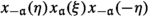, $\mathfrak {a}\in \Phi$, $\xi \in I$, $\eta \in R$. Some results in this direction are contained in the paper by Sinchuk and Smolensky [65]. As a more remote goal one could think of generalisations to birelative subgroups, see [33].

• Finally, there is a broader area of partial bounded generation, bounded generation in terms of other sets of generators, etc. When bounded generation in terms of X does not hold for the group G itself, one could ask, whether the width

  $$\begin{aligned} w_X(Y)=\sup l_X(g),\quad g\in Y, \end{aligned}$$

  is bounded, for certain subsets $Y\subseteq G$. For instance, the results by Stepanov and others that we mentioned in Sect. 3.9, imply that $w_{\textrm{E}}(C)$ is [uniformly] bounded for the set C of commutators in any Chevalley group of rank $\geqslant$ over an arbitrary commutative ring. Recently, the third author and Raimund Preusser established partial results in the same spirit for the set of $m^{\textrm{th}}$ powers. It is natural to expect that some form of this claim holds for arbitrary words, which would (in particular!) infer a negative answer to the problem of finite verbal width.

References

Abért, M., Lubotzky, A., Pyber, L.: Bounded generation and linear groups. Internat. J. Algebra Comput. 13(4), 401–413 (2003)
Adian, S.I., Mennicke, J.: Bounded generation of \({{\rm SL}}(n,{ Z})\). Internat. J. Algebra Comput. 2(4), 357–365 (1992)
Arlinghaus, F.A., Vaserstein, L.N., You, H.: Commutators in pseudo-orthogonal groups. J. Austral. Math. Soc. Ser. A 59(3), 353–365 (1995)
Aschenbrenner, M., Khélif, A., Naziazeno, E., Scanlon, T.: The logical complexity of finitely generated commutative rings. Int. Math. Res. Not. IMRN 2020(1), 112–166 (2020)
Avni, N., Lubotzky, A., Meiri, C.: First order rigidity of non-uniform higher rank arithmetic groups. Invent. Math. 217(1), 219–240 (2019)
Avni, N., Meiri, C.: Words have bounded width in \({\rm SL}(n,{\mathbb{Z} })\). Compositio Math. 155(7), 1245–1258 (2019)
Bass, H., Milnor, J., Serre, J.-P.: Solution of the congruence subgroup problem for \({\rm SL}_n (n\geqslant 3)\) and \({\rm Sp}_{2n} (n\geqslant 2)\). Inst. Hautes Études Sci. Publ. Math. 33, 59–137 (1967)
Behr, H.: Arithmetic groups over function fields. I: A complete characterization of finitely presented arithmetic subgroups of reductive algebraic groups. J. Reine Angew. Math. 495, 79–118 (1998)
Carter, D., Keller, G.: Bounded elementary generation of \({{\rm SL}}_n({{\mathscr {O}}})\). Amer. J. Math. 105(3), 673–687 (1983)
Carter, D., Keller, G.: Elementary expressions for unimodular matrices. Commun. Algebra 12(3–4), 379–389 (1984)
Carter, D., Keller, G.E.: Bounded elementary expressions in \({{\rm SL}}(2,{{\mathscr {O}}})\). Preprint, University of Virginia, 1–11 (1985)
Carter, D., Keller, G.E., Paige, E.: Bounded expressions in \({{\rm SL}}(2,{{\mathscr {O}}})\). Preprint, University of Virginia, 1–21 (1985)
Carter, R.W.: Simple Groups of Lie Type. Pure and Applied Mathematics, vol. 28. Wiley, London (1972)
Carter, R.W., Chen, Y.: Automorphisms of affine Kac–Moody groups and related Chevalley groups over rings. J. Algebra 155(1), 44–94 (1993)
Chang, C.C., Keisler, H.J.: Model Theory. 2nd edn. Studies in Logic and the Foundations of Mathematics, vol. 73. North Holland, Amsterdam (1977)
Cohn, P.M.: On the structure of the \({{\rm GL}}_2\) of a ring. Inst. Hautes Études Sci. Publ. Math. 30, 5–53 (1966)
Cooke, G.E.: A weakening of the Euclidean property for integral domains and applications to algebraic number theory. I. J. Reine Angew. Math. 282, 133–156 (1976)
Cooke, G.E.: A weakening of the Euclidean property for integral domains and applications to algebraic number theory. II. J. Reine Angew. Math. 283(284), 71–85 (1976)
Cooke, G., Weinberger, P.J.: On the construction of division chains in algebraic number rings, with applications to \({{\rm SL}}_2\). Commun. Algebra 3, 481–524 (1975)
Corvaja, P., Demeio, J., Rapinchuk, A., Ren, J., Zannier, U.: Bounded generation by semi-simple elements: quantitative results (2022). arXiv:2203.00755
Corvaja, P., Rapinchuk, A.S., Ren, J., Zannier, U.M.: Non-virtually abelian anisotropic linear groups are not boundedly generated. Invent. Math. 227(1), 1–26 (2022)
Demeyer, J.: Recursively enumerable sets of polynomials over a finite field are Diophantine. Invent. Math. 170(3), 655–670 (2007)
Dennis, R.K., Vaserstein, L.N.: On a question of M. Newman on the number of commutators. J. Algebra 118(1), 150–161 (1988)
Dennis, R.K., Vaserstein, L.N.: Commutators in linear groups. \(K\)-Theory 2(6), 761–767 (1989)
Ellers, E.W., Gordeev, N.: On the conjectures of J. Thompson and O. Ore. Trans. Amer. Math. Soc. 350(9), 3657–3671 (1998)
Erovenko, I.V.: \({{\rm SL}}_n(F[x])\) is not boundedly generated by elementary matrices: explicit proof. Electron. J. Linear Algebra 11, 162–167 (2004)
Erovenko, I.V., Rapinchuk, A.S.: Bounded generation of \(S\)-arithmetic subgroups of isotropic orthogonal groups over number fields. J. Number Theory 119(1), 28–48 (2008)
Ershov, M., Jaikin-Zapirain, A., Kassabov, M.: Property \((T)\) for Groups Graded by Root Systems. Memoirs of the American Mathematical Society, vol. 249(1186). American Mathematical Society, Providence (2017)
Estes, D., Ohm, J.: Stable range in commutative rings. J. Algebra 7, 343–362 (1967)
Garland, H.: The arithmetic theory of loop groups. Inst. Hautes Études Sci. Publ. Math. 52, 5–136 (1980)
Gvozdevsky, P.: Improved \({K}_1\)-stability for the embedding \(D_5\) into \(E_6\). Commun. Algebra 48(11), 4922–4931 (2020)
Gvozdevsky, P.: Bounded reduction of orthogonal matrices over polynomial rings. J. Algebra 602, 300–321 (2022)
Hazrat, R., Stepanov, A., Vavilov, N., Zhang, Z.: Commutator width in Chevalley groups. Note Mat. 33(1), 139–170 (2013)
Hodges, W.: Model Theory. Encyclopedia of Mathematics and its Applications, vol. 42. Cambridge University Press, Cambridge (1993)
Jordan, B.W., Zaytman, Y.: On the bounded generation of arithmetic \({{\rm SL}}_2\). Proc. Natl. Acad. Sci. USA 116(38), 18880–18882 (2019)
Kac, V.G.: Infinite-Dimensional Lie Algebras, 3rd edn. Cambridge University Press, Cambridge (1990)
Kharlampovich, O., Myasnikov, A.: What does a group algebra know about a free group. Ann. Pure Appl. Logic 169(6), 523–547 (2018)
Kharlampovich, O., Myasnikov, A., Sohrabi, M.: Rich groups, weak second-order logic, and applications. In: Kharlampovich, O., Sklinos, R. (eds.) Groups and Model Theory, pp. 127–193. de Gruyter, Berlin (2021)
Lenstra, H.W., Jr.: On Artin’s conjecture and Euclid’s algorithm in global fields. Invent. Math. 42, 201–224 (1977)
Liebeck, M.W., O’Brien, E.A., Shalev, A., Tiep, P.H.: The Ore conjecture. J. Eur. Math. Soc. (JEMS) 12(4), 939–1008 (2010)
Liebeck, M.W., O’Brien, E.A., Shalev, A., Tiep, P.H.: Commutators in finite quasisimple groups. Bull. London Math. Soc. 43(6), 1079–1092 (2011)
Liehl, B.: On the group \({{\rm SL}}_2\) over orders of arithmetic type. J. Reine Angew. Math. 323, 153–171 (1981)
Loukanidis, D., Murty, V.K.: Bounded generation for \({{\rm SL}}_n\) (\(n\geqslant 2\)) and \({\rm Sp}_{n}\) (\(n\geqslant 1\)) (1994). Preprint
Luzgarev, A.Yu., Stavrova, A.A.: The elementary subgroup of an isotropic reductive group is perfect. St. Petersburg Math. J. 23(5), 881–890 (2012)
Magurn, B.A.: Algebraic Introduction to \(K\)-Theory. Encyclopedia of Mathematics and its Applications, vol. 87. Cambridge University Press, Cambridege (2002)
Matsumoto, H.: Sur les sous-groupes arithmétiques des groupes semi-simples déployés. Ann. Sci. Éc. Norm. Sup. 2, 1–62 (1969)
Milnor, J.: Introduction to Algebraic \(K\)-Theory. Annals of Mathematics Studies, vol. 72. Princeton University Press, Princeton (1971)
Morgan, A.V., Rapinchuk, A.S., Sury, B.: Bounded generation of \({{\rm SL}}_2\) over rings of \(S\)-integers with infinitely many units. Algebra Number Theory 12(8), 1949–1974 (2018)
Morris, D.W.: Bounded generation of \({{\rm SL}}(n,A)\) (after D. Carter, G. Keller, and E. Paige). New York J. Math. 13, 383–421 (2007)
Murty, V.K.: Bounded and finite generation of arithmetic groups. In: Dilcher, K. (ed.) Number Theory (Halifax, NS, 1994). CMS Conference Proceedings, vol. 15, pp. 249–261. American Mathematical Society, Providence (1995)
Nica, B.: On bounded elementary generation for \({{\rm SL}}_n\) over polynomial rings. Israel J. Math. 225(1), 403–410 (2018)
Nies, A.: Separating classes of groups by first-order sentences. Internat. J. Algebra Comput. 13(3), 287–302 (2003)
Oger, F., Sabbagh, G.: Quasi-finitely axiomatizable nilpotent groups. J. Group Theory 9(1), 95–106 (2006)
O’Meara, O.T.: On the finite generation of linear groups over Hasse domains. J. Reine Angew. Math. 217, 79–108 (1965)
Peterson, D.H., Kac, V.G.: Infinite flag varieties and conjugacy theorems. Proc. Nat. Acad. Sci. USA 80(6), 1778–1782 (1983)
Platonov, V.P., Rapinchuk, A.S.: Abstract properties of \(S\)-arithmetic groups and the congruence problem. Russ. Acad. Sci. Izv. Math. 40(3), 455–476 (1993)
Plotkin, E.B.: Surjective stabilization for \(K_1\)-functor for some exceptional Chevalley groups. J. Soviet Math. 64(1), 751–766 (1993)
Plotkin, E.: On the stability of the \({\mathscr {K}}_1\)-functor for Chevalley groups of type \({ E}_7\). J. Algebra 210(1), 67–85 (1998)
Queen, C.: Some arithmetic properties of subrings of function fields over finite fields. Arch. Math. (Basel) 26, 51–56 (1975)
Rapinchuk, A.S.: The congruence subgroup problem for arithmetic groups of finite width. Soviet Math. Dokl. 42(2), 664–668 (1991)
Rapinchuk, A.S.: Representations of groups of finite width. Soviet Math. Dokl. 42(3), 816–820 (1991)
Roquette, P.: Class field theory in characteristic \(p\), its origin and development. In: Miyake, K. (ed.) Class Field Theory-its Centenary and Prospect (Tokyo, 1998). Advanced Studies in Pure Mathematics, vol. 30, pp. 549–631. Mathematical Society of Japan, Tokyo (2001)
Rosen, M.: Number Theory in Function Fields. Graduate Texts in Mathematics, vol. 210. Springer, New York (2002)
Segal, D., Tent, K.: Defining \(R\) and \(G(R)\), J. Europ. Math. Soc. https://doi.org/10.4171/JEMS/1255. arXiv:2004.13407
Sinchuk, S., Smolensky, A.: Decompositions of congruence subgroups of Chevalley groups. Internat. J. Algebra Comput. 28(6), 935–958 (2018)
Sivatski, A., Stepanov, A.: On the word length of commutators in \({\rm GL}_n(R)\). \({\mathscr {K}}\)-Theory 17(4), 295–302 (1999)
Smolensky, A.: Commutator width of Chevalley groups over rings of stable rank \(1\). J. Group Theory 22(1), 83–101 (2019)
Smolensky, A., Sury, B., Vavilov, N.: Gauss decomposition for Chevalley groups, revisited. Internat. J. Group Theory 1(1), 3–16 (2011)
Sohrabi, M., Myasnikov, A.G.: Bi-interpretability with \({ Z}\) and models of the complete elementary theories of \(SL_n({\mathscr {O}})\), \(T_n({\mathscr {O}})\) and \({\rm GL}_n({\mathscr {O}})\), \(n\geqslant 3\) (2020). arXiv:2004.03585
StackExchange discussion. https://math.stackexchange.com/questions/2690954/laurent-series-of-root-of-polynomials
Stein, M.R.: Generators, relations, and coverings of Chevalley groups over commutative rings. Amer. J. Math. 93, 965–1004 (1971)
Stein, M.R.: Surjective stability in dimension 0 for \(K_2\) and related functors. Trans. Amer. Math. Soc. 178, 165–191 (1973)
Stein, M.R.: Stability theorems for \({\mathscr {K}}_1\), \({\mathscr {K}}_2\) and related functors modeled on Chevalley groups. Japan J. Math. (N.S.) 4(1), 77–108 (1978)
Steinberg, R.: Générateurs, relations et revêtements de groupes algébriques. In: Colloq. Théorie des Groupes Algébriques (Bruxelles, 1962), pp. 113–127. Librairie Universitaire, Louvain (1962)
Steinberg, R.: Lectures on Chevalley Groups. University Lecture Series, vol. 66. American Mathematical Society, Providence (2016)
Stepanov, A.: Structure of Chevalley groups over rings via universal localization. J. Algebra 450, 522–548 (2016)
Stepanov, A., Vavilov, N.: On the length of commutators in Chevalley groups. Israel J. Math. 185, 253–276 (2011)
Tavgen, O.I.: Bounded generation of Chevalley groups over rings of algebraic \(S\)-integers. Math. USSR-Izv. 36(1), 101–128 (1991)
Thompson, R.C.: Commutators in special and general linear groups. Trans. Amer. Math. Soc. 101, 16–33 (1961)
Tits, J.: Uniqueness and presentation of Kac–Moody groups over fields. J. Algebra 105(2), 542–573 (1987)
Trost, A.A.: Bounded generation by root elements for Chevalley groups defined over rings of integers of function fields with an application in strong boundedness (2021). arXiv:2108.12254
Trost, A.A.: Elementary bounded generation for \({{\rm SL}}_n\) for global function fields and \(n\geqslant 3\) (2022). arXiv:2206.13958
van der Kallen, W.: \({{\rm SL}}_3({\mathbb{C} }[X])\) does not have bounded word length. In: Dennis, R.K. (ed.) Algebraic K-theory, Part I (Oberwolfach 1980). Lecture Notes Mathematics, vol. 966, pp. 357–361. Springer, Berlin (1982)
Vaserstein, L.N.: Bounded reduction of invertible matrices over polynomial rings by addition operations. Preprint, Pennsylvania State University (2006). http://www.personal.psu.edu/lxv1/pm2.pdf
Vaserstein, L.N.: Polynomial parametrization for the solution of Diophantine equations and arithmetic groups. Ann. Math. 171(2), 979–1009 (2010)
Vaserstein, L.N., Wheland, E.: Commutators and companion matrices over rings of stable rank \(1\). Linear Algebra Appl. 142, 263–277 (1990)
Vavilov, N.: Structure of Chevalley groups over commutative rings. In: Yamaguti, K., Kawamoto, N. (eds.) Nonassociative Algebras and Related Topics (Hiroshima, 1990), pp. 219–335. World Scientific Publishing, River Edge (1991)
Vavilov, N., Plotkin, E.: Chevalley groups over commutative rings. I: Elementary calculations. Acta Appl. Math. 45(1), 73–113 (1996)
Vavilov, N.A., Smolensky, A.V., Sury, B.: Unitriangular factorizations of Chevalley groups. J. Math. Sci. (N.Y.) 183(5), 584–599 (2012)
Vsemirnov, M.: Short unitriangular factorizations of \({{\rm SL}}_2({\mathbb{Z} }[1/p])\). Q. J. Math. 65(1), 279–290 (2014)
Acknowledgements
Very special thanks go to Inna Capdeboscq. This paper started jointly with her as a discussion of the bounded commutator width of various classes of Kac–Moody groups over finite fields, and for a long time it was supposed to be a work of four authors. Our sincere thanks go to Nikolai Gordeev, Olga Kharlampovich, Jun Morita, Alexei Myasnikov, Denis Osipov, Alexei Stepanov, and Igor Zhukov for useful discussions regarding various aspects of this work. We thank the referees for careful reading and meticulous remarks.
Author information
Authors and Affiliations
Corresponding author
Additional information
In memory of Irina Suprunenko, our dear friend and colleague.
Publisher's Note
Springer Nature remains neutral with regard to jurisdictional claims in published maps and institutional affiliations.
Research of Boris Kunyavskiĭ and Eugene Plotkin was supported by the ISF Grants 1623/16 and 1994/20. Nikolai Vavilov thanks the “Basis” Foundation Grant N. 20-7-1-27-1 “Higher Symbols in Algebraic K-Theory”
Rights and permissions
Springer Nature or its licensor (e.g. a society or other partner) holds exclusive rights to this article under a publishing agreement with the author(s) or other rightsholder(s); author self-archiving of the accepted manuscript version of this article is solely governed by the terms of such publishing agreement and applicable law.
About this article
Cite this article
Kunyavskiĭ, B., Plotkin, E. & Vavilov, N. Bounded generation and commutator width of Chevalley groups: function case. European Journal of Mathematics 9, 53 (2023). https://doi.org/10.1007/s40879-023-00627-y
Received:
Revised:
Accepted:
Published:
DOI: https://doi.org/10.1007/s40879-023-00627-y