
Abstract
The aim is to describe two homogeneous affine open sets in some projective spaces. The sets are well known, their groups of automorphisms contain simple exceptional groups of types \(E_6\) or \(E_7\), although the total groups of automorphisms are infinite-dimensional and both the sets are flexible. We prove existence of automorphisms not belonging to the connected components of unity, construct extended Weyl groups including these non-tame automorphisms. Our methods are based on classical combinatorics associated with 27 lines on non-singular cubic surfaces and with 56 exceptional curves on Del Pezzo surfaces of degree 2. Some traditional applications of Jordan algebras are used.
1 Introduction: a model example
Assume the ground field K is algebraically closed and its characteristic is not equal to 2 or 3.
Definition 1.1
An affine open set in the projective space \({\mathbb {P}}^N\) is a complement of a hypersurface.
If the hypersurface is defined by a homogeneous equation  , then we denote it by the symbol [f], so its complementary affine set is
  .
.
Definition 1.2
([1]) An irreducible non-singular affine variety of dimension greater than 1 is flexible if the tangent space at any point of the variety is generated by the fields of velocity for actions of one-parameter additive subgroups of the automorphism group of the variety.
The authors of [1] have demonstrated that such a variety has an infinitely dimensional and m-transitive group of automorphisms for every natural m.
A preliminary remark about the study of examples. Certainly, there are a lot of flexible affine sets where some classical simple linear groups (or direct products of such groups) act transitively. For instance, in the projectivizations of the entry spaces of variable square (resp. symmetric, skew) matrices, open sets which are complements to the zeros of determinant (resp. discriminant, Pfaffian) are flexible, but our further attention will be paid mainly to two exceptional groups \(E_6,E_7\), their special homogeneous spaces, the first of which is the complement of a cubic hypersurface in \({\mathbb {P}}^{26}\), the second one is the complement of a quartic hypersurface in \({\mathbb {P}}^{55}\). Nevertheless the case of Pfaffian as an introductory thing will be considered in more detail below, in Example 1.3.
The corresponding cubic form of 27 variables and quartic form of 56 variables are well known, the cubic form (at least for the case of characteristic 2 of the ground field) was written down by Camille Jordan in 1870 (see [13, 3rd line at the top, p. 317]). We indicate Jordan as a predecessor of study of the cubic form, because nobody mentions him in that context. Both the forms were studied by use of combinatorics of some objects of algebraic geometry, they are 27 lines on a cubic surface and 56 exceptional curves on Del Pezzo surface of degree 2 or 28 bitangents of a plane quartic curve. For example see Remark 5.9 where a generalized Cayley–Salmon bifid transformation is described. Moreover, there are tight and well-known connections of \(E_6,E_7\) with (Pascual) Jordan algebras. We will use them together with the mentioned algebro-geometric combinatorics in our proofs and constructions, especially in elementary proofs of flexibility (Proposition 3.7, Theorem 4.3), in descriptions of non-tame automorphisms (Definitions 3.9, 4.4, Theorems 3.11, 4.5). These involutive automorphisms are also well known, but as it seems nobody considered them from the point of view of non-tameness. Non-tameness of an automorphism means that it does not belong to the connected component of the identity automorphism, connectedness is considered in ind-topology. A description of the topology and other basic definitions of the theory of infinite-dimensional groups were introduced in the opening part of the article [19] by Shafarevich. Moreover our techniques allow to include these involutions in extended Weyl groups, see Propositions 3.12, 5.10 and subsequent Remarks 3.13, 5.11.
Example 1.3
Here we consider the Pfaffian determinant as a good introductory sample.
(a) Let U be a  matrix, assume that it is skew and zero-axial, let \(u_{ij}, 1\leqslant i<j\leqslant 2n\), be its entries disposed over the principal diagonal. The determinant of U is the square of a polynomial of order n of the entries,
  . The last identity determines the Pfaffian up to a sign, therefore the Pfaffian is normalized by the condition that the primitive monomial
  of
of  is taken with coefficient \((+\,1)\). Equivalently the Pfaffian of U is defined by the equality

the sum is taken over all presentations of  as a disjoint union of n pairs,
  , ...,
  , and
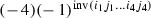
, and  is the number of inversions in permutation
  . Note that the evenness of the number does not depend on the order of the pairs. Totally the Pfaffian has \((2n-1)!!\) terms.
(b) For small n the signs at primitive monomials of general Pfaffian  can be described as follows. Let us take a convex plane 2n-polygon with vertices marked by numbers \(1,2,\dots ,2n\) clockwise arranged around an oval. The primitive monomial
  , \(i<j\), \(k<l\), ..., \(p<q\), can be represented as the union of segments
  having ends among the mentioned vertices. Its sign is plus if the number of mutual intersections of the segments is even, and the sign is minus if the number is odd.
An illustration of the simplest case \(n=2\) is the following 3-termed expansion of

Three monomials taken from  , \(n=3\), are pictured below:

Case \(n=4\), one example of monomial with the plus sign:

A simple corollary of these pictures is that the circular permutation \((1,2,\dots , 2n-1,2n)\) of indices of variables \(u_{ij}\) (and the iterations of the permutation) induces a substitution of the variables preserving the Pfaffian of skew matrix U, that is the linear substitution

where the addition modulo 2n is applied, the Pfaffian is unaltered by the action of rotation R.
(c) The number of independent entries in U is equal to  , so a non-zero skew matrix determines a point in \({\mathbb {P}}^N\), where
  . Actions \(U\mapsto A^{\texttt {T}}UA\) with non-degenerate
  matrices A preserve the space of skew matrices and preserve their Pfaffians (up to a non-zero multiplier). This action of
  is transitive on the set of non-degenerate skew
  matrices. Among the matrices
  , there is a sufficiently large number of one-parameter additive subgroups defined by elementary unipotent matrices, therefore the open affine set
  is flexible.
An automorphism is tame if it belongs to the connected component of the identity automorphism, connectedness is considered from the point of view of ind-topology. Below we prove existence of non-tame automorphism of this affine set for the case \(n>2\).
(d) If the matrix elements \(u_{ij}\) are considered as variables, then the Pfaffian is a homogeneous form of n-th order of the variables. One can take the matrix gradient of the Pfaffian function, that is

The above partial derivative \(s_{ij}\) equals the Pfaffian (taken with sign \((-1)^{i+j+1}\)) of  skew matrix \(U_{ij}\) produced by deleting two rows and two columns of U marked by numbers i, j.
The following two properties of the gradient take place:

These identities are consequences of the corresponding properties of ordinary determinants applied to skew  matrices. It follows that the map
  is an involutive automorphism of the open affine set
  . The Picard group of the affine open set
  (see Definition 1.1), where f is an irreducible form of degree d, is isomorphic to \({\mathbb {Z}}_d\), but elements of the connected component of the identity induce trivial actions on the finite Picard group because any element of such a component can be deformed continuously to the identity transformation along the component. The gradient transformation being defined by forms of degree \(n-1\) acts on the group
  (isomorphic to \({\mathbb {Z}}_n\)) as the multiplication by \((-1)\). So the assertion about non-tameness of the gradient transformation is proved. The above gradient construction and the proof constitute a model of some our future considerations, e.g., Theorems 3.11, 4.5.
(e) A few words about an extended Weyl group for this example. The simple linear group  of type \(A_{2n-1}\) acts on \({\mathbb {P}}^N\), preserves the hypersurface
  and its complement. A maximal (and
  -dimensional) torus \({\mathbb {T}}\) in the group consists of elements whose representatives in
  are diagonal matrices
  , \(\lambda _i\in K^*\). The Weyl group is the normalizer of \({\mathbb {T}}\), there is a natural set of coset representatives (modulo \({\mathbb {T}}\)) in the normalizer. These representatives are permutations of indices \(1,2,\dots ,2n\), the permutations induce corresponding substitutions of variables \(u_{ij}\), these substitutions can be considered as projective transformations preserving
  . So we have automorphisms of the open affine set
  which can be identified with elements of the Weyl group. One can extend this group adding the above gradient transformation (as an additional generator). It is not hard to see that this transformation normalizes \({\mathbb {T}}\).
(f) Finally, about a combinatorics and its connection with the Coxeter–Dynkin constructions. For a semisimple group G, roots are vectors in some Euclidean (or hyperbolic) space. A projective root is a root considered up to proportionality, to speak plainly, projective root is the pair  , where e is a root. There is a partial operation of addition for projective roots: sum of
  and \(\{f, -\,f\}\) is defined and equal to
  if one of sums
  is a root g or
  . The projective roots of the algebraic group constitute a graph \(\mathrm{\Gamma }(G)\): two roots with defined addition between them are adjacent in \(\mathrm{\Gamma }(G)\). Certainly, the Weyl group W(G) of G acts naturally on the graph. In this example we consider the action of \(W(A_{2n-1})\) on \(\mathrm{\Gamma }(A_{2n-1})\).
For the case of Pfaffian one can consider the so-called double  -sets consisting of
  distinct variables belonging to the set
  , such that there exists their ordering \(x_1,\dots , x_{2n-2}, y_1,\dots , y_{2n-2}\) and the following properties hold: every product
  , \(1\leqslant i,j\leqslant 2n-2\), is not a sub-monomial of any non-zero monomial from the expansion of
  , but every product
  , \(1\leqslant i,j\leqslant 2n-2, i\ne j\), is a part of a non-zero monomial. One can construct a graph \(\mathrm{\Gamma }\) whose vertices are double
  -sets, two vertices are adjacent if the symmetric difference of these double
  -sets is again a double
  -set. Certainly, the Weyl group \(W(A_{2n-1})\) acts on the graph, more precisely the above mentioned permutations (see (e)) act. Moreover graphs \(\mathrm{\Gamma }\) and \(\mathrm{\Gamma }(A_{2n-1})\) are isomorphic, the isomorphism is \(W(A_{2n-1})\)-equivariant. Below a short explanation is given.
Every double  -set can be marked by the symbol
  . For example

The total number of double  -sets is
  , it coincides with the number of projective roots for \(A_{2n-1}\). Two double
  -sets
-sets  and
and  are adjacent if
  and
and  have exactly one common element. In such a case,
  . Now, a one-to-one \(W(A_{2n-1})\)-equivariant correspondence between two graphs is obvious: the transposition
  (more precisely, the projective root determined by the transposition) corresponds to the double
  -set
-set  . Below a subgraph corresponding to the Dynkin diagram for \(A_{2n-1}\) is shown. It is

Basic projective roots correspond to the subgraph vertices. Generation of other projective roots with the help of partial addition and generation of other double  -sets with the help of partial symmetric differences go in parallel paths.
2 Cubic form \(F_3\) of 27 variables
The set of 27 variables will be subdivided into three parts, that is, \(v_i\), \(1\leqslant i \leqslant 6\),  , \(1\leqslant j \leqslant 6\), and , \(1\leqslant p,q\leqslant 6\), \(p<q\). The variables constitute an ordered set (or a variable vector) which is denoted by \(\mathbf{{a}}\),

where the meaning of 6-vectors \(\overline{v},\overline{w} \) or of 15-vector \(\overline{u}\) is clear. Moreover, the big letter U will be used for the  skew matrix whose elements over the principal diagonal are
  . Sometimes we will use additional ordered sets \(\mathbf{{b}},\mathbf{{c}}\) of either parallel variables or some other quantities,
The inner product \((\mathbf{{a}},\mathbf{{b}})\) of two vectors \(\mathbf{{a}},\mathbf{{b}}\) is defined by

cubic form \(F_3\) of 27 variables  is defined by

where the first summand is

the second one is the Pfaffian determinant of U. The detailed expansion is

The form contains 45 monomial terms.
Now let us recall the notion of the gradient vector and its linearization (see also Definition 3.9 where another name for the gradient transformation is given, and historic explications in Remarks 3.10).
Definition 2.1
For the form \(F_3(\mathbf{{a}})\), its gradient \(\nabla _\mathbf{{a}} F_3(\mathbf{{a}})\) is the vector \(\mathbf{{c}}\) whose coordinates are partial derivatives, that is

We will write \(\mathbf{{a}}^{\#}\) instead of \(\nabla _\mathbf{{a}} F_3(\mathbf{{a}})\).
The bilinearization of quadratic polynomials taken as the coordinates of the gradient produces formulas for a symmetric multiplication  , that is

Lemma 2.2
The following identities take place:

Proof
They are modifications of similar formulas from texts by Brown [3], Freudenthal [6,7,8], McCrimmon [16], and Springer–Veldkamp [20]. \(\square \)
Corollary 2.3
Let \(\mathrm{\Pi }\) be the “kernel” of the sharp operation, that is

If \(\mathbf{{c}}\in \mathrm{\Pi }\) and \(\mathbf{{a}},\mathbf{{b}} \) are arbitrary 27-vectors, then

Proof
These consequences are obvious. \(\square \)
The form \(F_3\) (as well as some other cubic forms like the determinant of  matrix, the Pfafian of
  skew matrix or cubic determinant of
  matrix) satisfies the following properties:
-
(i)
It does not contain monomials with cubes or squares of variables.
-
(ii)
For any couple of distinct variables there exists at most one non-zero monomial containing the product of these two variables.
For a cubic form f of n variables satisfying properties (i), (ii), it is reasonable to construct a square  symmetric incidence matrix
  whose rows and columns are marked by the variables, the element standing in the x-row and y-column equals r if rxyz is a monomial from the expansion of f (if such a monomial does not exist then \(r=0\)).
For our form \(F_3\), the entries of the  matrix
  belong to
  . The principal
  submatrix of
  corresponding to the last 15 rows and last 15 columns is
  . The matrix
  is shown in Appendix.
Remark 2.4
More generally, for any cubic form f of n variables (maybe without properties (i), (ii)),  is the matrix of multiplied by 2 quadratic form equal to the sum of n first partial derivatives of f. Maybe the Hessian matrix
  with xy-elements \(\partial ^2 f/\partial x \partial y\) is more informative than
  , but we will not use such matrices.
Remark 2.5
If one omits the signs, then the incidence matrix of 27 lines of a non-singular cubic surface arises. If its rows and columns are ordered as variables in \(\mathbf{{a}}\), then  with entries taken without signs coincides with the incidence matrix shown in Henderson [11, p. 24].
Definition 2.6
For two ordered sets of cardinality n,  and \(\mathbf{{y}}=(y_1,\dots ,y_n) \) such that \(\{ x_1,\dots ,x_n\} ,\{ y_1,\dots ,y_n\}\subset \mathbf{{a}} \) (the set \(\mathbf{{a}}\) is taken unordered in two last inclusions) the incidence
  submatrix \(m(\mathbf {x},\mathbf {y})\) of the matrix
  has n rows marked by elements of the ordered set \(\mathbf{{x}}\) (the order of rows is defined by the order in \(\mathbf{{x}}\)), columns marked by elements of the ordered set \(\mathbf{{y}}\), every entry of \(m(\mathbf {x},\mathbf {y})\) coincides with the corresponding entry of
  . Submatrices of type \(m(\mathbf {x},\mathbf {x})\) are called principal submatrices of
  , although they are produced by interchange of some rows and columns of standard principal submatrices.
Remark 2.7
Non-zero 45 monomials rxyz of \(F_3(\mathbf{{a}})\) correspond to triangles, i.e., to tritangent planes of the cubic surface. Any triangle determines a principal  submatrix (see Definition 2.6)
  (where \(\mathbf{{t}}=(x,y,z)\)) of
  with zero diagonal and non-zero number r,
  , out the diagonal.
Definition 2.8
The double six is a collection of 12 distinct variables \(x_1,\dots ,x_6, y_1,\dots , y_6 \) taken from the above 27 variables such that there are orderings, say , \(\mathbf{{y}}=(y_1,\dots ,y_n)\), producing  vanishing principal submatrices \(m(\mathbf {x},\mathbf {x})\), \(m(\mathbf {y},\mathbf {y})\) (see Definition 2.6), submatrix \(m(\mathbf {x},\mathbf {y})\) with zero principal diagonal (that is
  if \({1\leqslant i\leqslant 6}\)), but every element of \(m(\mathbf {x},\mathbf {y})\) out the principal diagonal is not zero (that is
  ), cf. [11, p. 16].
Sometimes, for the double six we will use the notation
Any simultaneous permutation of indices of variables x, y from a double six produces a double six, which will be identified with initial one. We will choose (together with Henderson [11, p. 23]) one representative from each collection of permutationally equivalent double sixes.
Remark 2.9
There are 36 distinct double sixes, see [11, p. 23]. They correspond to projective roots of \(E_6\) (see Example 1.3 (f)). Existence of a one-to-one correspondence is obvious, because there are 72 roots for \(E_6\), but the correspondence established below preserves some geometric interrelations among the set of roots and combinatorial connections between the double sixes, the correspondence is \(W(E_6)\)-equivariant.
Definition 2.10
The graph \(\mathrm{\Gamma } (E_6)\) with a partial operation on the set of its vertices is a particular case of the graph defined in Example 1.3 (f) for any semisimple group. \(W(E_6)\) acts on \(\mathrm{\Gamma } (E_6)\).
Definition 2.11
The graph \(\mathrm{\Gamma }(DS)\), whose vertices are double sixes with a partial operation on the set of vertices is defined as follows (also cf. Example 1.3 (f)): Two double sixes are adjacent if the symmetric difference of these double sixes can be presented as a double six, that is if the symmetric difference contains 12 variables, and these variables can be ordered as in Definition 2.8. The operation of symmetric difference is partial, it is denoted by the standard symbol \(\triangle \).
Theorem 2.12
There exists an isomorphism between graphs \(\mathrm{\Gamma } (E_6)\) and \(\mathrm{\Gamma }(DS)\). Moreover, there exists an action of \(W(E_6)\) on \(\mathrm{\Gamma }(DS)\) such that the isomorphism is \(W(E_6)\)-equivariant.
Proof
Let us begin with the list of double sixes. At the left hand sides, some of our notations for double sixes are written down, at the right hand sides, Henderson’s notations [11] are reproduced.

where i, j, \(a< b<c<d\),  , and
, and  .
.
Further,

where \(i<j<k\), \(a<b<c\),  .
.
Symmetric differences between the above double sixes are the following. If \(i<j<k\), then

If \(i< j<k\), \(a< b< c\),  , then

The subgraph generated by six double sixes
is a \(E_6\)-like thing
One can identify \(e_1,\dots ,e_6\) with basic positive roots of \(E_6\) arising from the Coxeter–Dynkin diagram. All other 30 double sixes are expressible via the basic \(e_1,\dots ,e_6\) with the help of symmetric difference, all 30 non-basic projective roots have parallel expressions in the terms of basic projective roots.
Indeed, for  we see

Further, if \(2\leqslant i<j<k\leqslant 6\), then

At last,
The double six at the left hand side corresponds to the maximal (with respect to \(e_1,\dots , e_6\)) root
where the addition operation is applied to positive basic vector roots \(e_1,\dots ,e_6\), but an expression of the double six with the help of symmetric differences connecting the basic six double sixes needs some accuracy. Indeed, this commutative binary operation is partial (that is not defined for every pair), not necessary associative, because after change of brackets the indefiniteness arises sometimes.

So we see a complete parallelism between the projective roots, their partial sums and double sixes with their partial symmetric differences.
Briefly about a Weyl-equivariance. For a non-singular cubic surface, the Picard group tensorially multiplied by \({\mathbb {Q}}\) and endowed with the inner hyperbolic product induced by the intersection number is the place of roots. \(W(E_6)\) acts on the Picard group. All the combinatorial connections in both the graphs and the partial operations are \(W(E_6)\)-equivariant. See [14, Chapter IV].\(\square \)
Remark 2.13
For a further application in Proposition 3.13, it is necessary to add some details on an action of \(W(E_6)\) (more precisely, actions of some coset-representatives modulo a maximal torus in its normalizer) on  .
.
Generally, the Weyl group of a semisimple linear algebraic group is the quotient group of the normalizer of a maximal torus by the torus. We consider the group of linear transformations preserving the cubic form \(F_3\) and its toric subgroup \({\mathbb {T}}\) consisting of linear substitutions expressible as multiplications of variables from the set  of 27 variables by non-zero constants and preserving (up to a multiplier) the cubic form \(F_3\). Any element of such a torus is completely determined by the action of the element on variables \(v_i\), the element multiplies \(v_i\) by \(\lambda _i\in K^*\), action of the element on other variables is enforced:

It is obvious that these transformations preserve \(F_3\), and the maximal torus \({\mathbb {T}}\) is projectively 6-dimensional. Let \({\mathbb {N}}\) be the normalizer of \({\mathbb {T}}\) in the group of linear transformations projectively preserving \(F_3\). Moreover, we will use the sign changing subgroup \(S{\mathbb {T}}\) of \({\mathbb {T}}\) consisting of the above elements with \(\lambda _i\in \{+1,-1\}\), and sign changing subgroup \(S{\mathbb {N}}\) of the normalizer \({\mathbb {N}}\).

It is clear that \(S{\mathbb {T}}\) is an invariant subgroup of \(S{\mathbb {N}}\), that \(S{\mathbb {T}}\) is an elementary Abelian 2-group isomorphic to \({\mathbb {Z}}_2^6\). It is possible to generate \(S{\mathbb {N}}\) by some involutive elements corresponding to double sixes.
Every double six s determines a transformation  such that \(T_s\) preserves the set of variables from s (up to signs of these variables), interchanges double sixes (more precisely, the sets of variables taken without signs), \(T_s^2\in S{\mathbb {T}}, T_s^4=1\).
Explicit description of \(T_s\) for double sixes s is as follows. \(T_{\langle 123456\rangle }\) is defined by formulas

Transformations \(T_{\langle pq\rangle }\), \(1\leqslant p<q\leqslant 6\), are defined by

where we assume that \(1\leqslant i\leqslant 6\), \( i\ne p, i\ne q\),  , \(u_{qi}=u_{iq}\), and all other variables are fixed by \(T_{\langle pq\rangle }\).
Now, as for involution (modulo the torus)  corresponding to
  . Assume that \(i<j<k\), \(a<b<c\),
  . Defining formulas for
  are
are

where equality  is assumed for cases where
  , . It is not hard to verify the Weyl-group properties of the transformations, that is involutiveness modulo the subgroup \(S{\mathbb {T}}\) of the above transformations. Moreover, products
  ,
,  ,
,  ,
,  are also involutive modulo \(S{\mathbb {T}}\), and the third powers of products ,
  ,
,  ,
,  ,
,  , belong to \(S{\mathbb {T}}\): the product of two transformations corresponding to two double sixes connected by edge in \(\mathrm{\Gamma }(DS)\) is an element of the third order modulo \(S{\mathbb {T}}\).
So we see that  .
.
Now it is clear that the above transformations \(T_s\) act on the set of double sixes, these transformations preserve the graph structure of \(\mathrm{\Gamma }(DS)\), \(W(E_6)\)-actions on the set of projective roots and on the set of double sixes are bilaterally matched.
Remark 2.14
If \({\Lambda }\in {\mathbb {T}} \) is the general toric element mentioned in the above remark, the element defined by numbers \(\lambda _1, \dots ,\lambda _6\) and  , then
Remark 2.15
As a preface to the next sections, one can say about another well-known construction of \(F_3\), where instead of Pfaffian, ordinary determinants of three  matrices are used. If these matrices X, Y, Z are respectively

then

If \(F_3\) is given in such a form, and for a matrix A, \((A)_{ij}\) denotes its ij entry, \(A^*\) denotes its adjoint, then new three  matrices \(X',Y',Z'\) defining the gradient vector \(\mathbf{{a}}^{\#}\) have entries defined as follows:
Actions

of non-degenerate  matrices A preserve \(F_3\) up to non-zero multipliers. For example, simultaneous conjugations by unipotent matrices of the form

where or or  , produce actions of one-parameter additive group with parameter \(\tau \).
3 Description of essentially the same cubic form by means of the split Albert Jordan algebra: flexibility, non-tameness
First of all, it is necessary to define the Zorn vector-matrix algebra. Another name for the algebra is split octonions.
A short definition of split octonions is given in McCrimmon’s book [16, p. 66], but below, in Definition 4.1, we will need a variation of such a definition, therefore some details (presented in [16, p. 158]) are written here.
Definition 3.1
The Zorn vector-matrix algebra consists of  matrices with scalar entries \(\alpha , \beta \in K\) on the principal diagonal and vector entries
  , \(\mathbf{{y}}=(y_1, y_2, y_3)\in K^3\) off the diagonal:

The componentwise operation of addition is natural in  . The multiplication is defined by

where ordinary dot and cross vector products are used, that is

Some K-valued functions on  are defined with the help of conjugation (adjunction),

The conjugation is linear and multiplicatively anti-isomorphic, that is

The mentioned functions are  and
and  are
are

Let \(\tau \) be a non-zero element of the ground field K. We say that an element Z of the Zorn algebra is \(\tau \)-basic, if one of eight field elements \(\alpha ,\beta , x_1,x_2,x_3, y_1, y_2, y_3 \) equals \(\tau \), but all other seven elements are zeros. Note that the function  vanishes on the set of \(\tau \)-basic elements.
A description of Albert’s exceptional 27-dimensional split Jordan algebra is given below. The Zorn algebra and the conjugation in it will be used, especially, the word “Hermitian” means Hermitian with respect to Zorn’s conjugation.
Definition 3.2
The Albert algebra is the algebra of  Hermitian matrices with entries in the Zorn algebra. The Albert algebra is endowed with the product
  , where AB is the ordinary matrix product. More precisely, Hermitian
  matrices have scalar entries
  on the principal diagonal and Zorn’s entries \(Z, Z', Z'', {\overline{Z }}, {\overline{Z'}}, {\overline{Z''}} \) disposed as one can see below,
Another standard notation for such a matrix is

Multiplication is the symmetrization of an accurate multiplication in the algebra of  matrices (with substitutions of scalars \(\lambda \in K\) instead of \(\lambda E_2\) in the entries arising in the principal diagonal), that is

where

The norm cubic form promised in the title of the section is defined by

where  and
and  are described in Definition 3.1.
Remark 3.3
Another description of the cubic norm is as follows:

where
Lemma 3.4
There exists a substitution of variables (taken with some signs) transferring \(F_3\) to N.
Proof
It is sufficient to compare Remarks 3.3 and 3.5.\(\square \)
Remark 3.5
(particularly formula (3)) Certainly, a substitution from Lemma 3.4 is not unique because of existence of some elementary automorphisms of both the forms.
Remark 3.6
According to the description of multiplication in Definition 3.2, right multiplication by the element of the form  (see notation (5)), where one component of the triplet \(( V, V', V'')\) is \(\tau \)-basic according to the end of Definition 3.1 and two other components are zeros, produces an action of one-parameter additive group (with parameter \(\tau \)) on the Albert algebra, the action preserves the norm cubic form. Taking corresponding vector fields on the Albert algebra, we obtain 24 linearly independent vectors at the unit point
  (see notation (5)).
Proposition 3.7
The complement of the cubic hypersurface \([F_3]\) in \({\mathbb {P}}^{26}\) is flexible.
Proof
The homogeneity follows from the opportunity of multiplication by elements with non-zero norm in the Albert algebra. Indeed, in this algebra every element with non-zero norm is invertible, so one can move every element to e. It is sufficient to show that there are 26 (or 27 if we consider the cone in \({\mathbb {A}}^{27}\) over our projective set) linearly independent in point e locally nilpotent vector fields. According to Remark 3.6, we already have 24 such fields. In Remark 2.15, formula (4), we have seen three other fields. Linear independence in point e of these 27 vector fields is evident.\(\square \)
Remark 3.8
One can obtain Proposition 3.7 as a corollary of [1, Theorem 5.6], but our consideration of a special case of this theorem is comparatively elementary.
Definition 3.9
Freudenthal’s quadratic transformation of 26-dimensional projective space is the 27-dimensional sharp transformation \(\mathbf{{a}}\mapsto \mathbf{{a}}^{\#}\) from Sect. 2, Definition 2.1.
Remark 3.10
Note that the sharp transformation was discovered by Freudenthal in the context of the Albert (non-split) Jordan algebra. See [9, 10, pp. 196–197, 2.6–2.12, formula (4.7)]). Moreover, Freudenthal studied the bilinearization of the transformation, later named as cross-product  or sharp product
  , [9, 10, pp. 199–200, formula (7.1)]. See also [20, pp. 75–76, 80–81], where the fundamental set of this quadratic birational transformation is described.
According to Jacobson [12, p. 232], for an element X of the Albert algebra (see Definition 3.2) the transformation is given by

Theorem 3.11
The Freudenthal transformation is a non-tame automorphism of the affine set  .
.
Proof
A universal reasoning was presented by consideration of the Pfaffian example in Example 1.3 (c). It fits for our case.\(\square \)
Proposition 3.12
The Freudenthal transformation normalizes the maximal torus.
Proof
It follows from immediate verification using explicit formulas for the action of torus (they are presented in Remarks 2.13, 2.14) and formulas for the quadratic (sharp) transformation (see identities (2)).\(\square \)
Remark 3.13
The quadratic transformation taken together with involutions described in Remark 2.13 generate a subgroup \({\widetilde{\mathbb {N}}}\) in the group of automorphisms of the affine set, the quotient group \({\widetilde{\mathbb {N}}}/{\mathbb {T}}\) is finite and may be considered as an extended Weyl group. Note that the number of elements of the extended Weyl group is equal to \(2\vert W(E_6)\vert \).
4 A quartic form of 56 variables consisting of 1036 monomials
A variant of Zorn’s construction. The idea is taken from [3, p. 87], opening paragraphs of Sect. 3. We consider a variant of Zorn’s construction for the case where a cross product is commutative.
Definition 4.1
Let B be any commutative (but not necessary associative or alternative) n-dimensional algebra over the basic field K, assume that multiplication in the algebra is noted as cross-product,  , and that B is endowed with an inner product
  with values in K. The new vector space \({ Z }(B)\) of dimension
  endowed with a multiplication-like binary operation (but not necessary commutative or associative), a quadratic form f and a biquadratic form q are defined as follows.
\({ Z }(B)\) consists of  matrices with scalar entries \(\alpha , \beta \in K\) on the principal diagonal and entries \(\mathbf{{a}}\in B, \mathbf{{b}}\in B\) off the diagonal:

In \({ Z }(B)\), the componentwise operations of addition or multiplication by a scalar are natural. The quadratic form f is defined by

The multiplication is defined by

that is the operation is similar to multiplication in the Zorn algebra.
There are three involutive linear transformations of \({ Z }(B)\), they are \({\texttt {R}}, {\texttt {S}}\) and \({\texttt {adj}}\).
-
(i)
\({\texttt {R}}\) is the reflection with respect to the matrix center,
$$\begin{aligned} \left( \begin{array}{cc} \alpha &{} \mathbf{{a}} \\ \mathbf{{b}}&{} \beta \end{array} \right) ^{{} \texttt {R}}=\left( \begin{array}{cc} \beta &{} \mathbf{{b}} \\ \mathbf{{a}}&{} \alpha \end{array} \right) , \end{aligned}$$it preserves the binary operation of multiplication,
 ,
, -
(ii)
\({\texttt {S}}\) is the transposition with respect to the secondary diagonal:
$$\begin{aligned} \left( \begin{array}{cc} \alpha &{} \mathbf{{a}} \\ \mathbf{{b}}&{} \beta \end{array} \right) ^{{} \texttt {S}}=\left( \begin{array}{cc} \beta &{} \mathbf{{a}} \\ \mathbf{{b}}&{} \alpha \end{array} \right) , \end{aligned}$$it is a multiplicative anti-isomorphism, that is
 .
. -
(iii)
\({\texttt {adj}}\) is the formation of adjoint
 matrix,
 ,
, .
. matrix,
The biquadratic form q is defined by the chain of the following three equalities:
Forms \(q_1,q_2\) are without good invariant properties, but their linear combination q is a good invariant. A more detailed description of \(q_1,q_2,q\) is

so

Definition 4.2
It is a specialization of Definition 4.1. Let us take a split Albert algebra A with the inner product induced by the bilinearization quadratic of the quadratic form
see Definitions 3.2, 3.1, where the multiplication in the Albert algebra and the function  are defined. Notation \({ Z }(A)\) will be used for the 56-dimensional vector space taken together with all additional structures from Definition 4.1 applied to the case \(B=A\).
Theorem 4.3
The complement of the quartic hypersurface  in \({\mathbb {P}}^{55}\) is flexible.
Proof
Results and ideas of Robert Brown presented in [3] will be used in the proof. First of all, he proved that the set is homogeneous [3, Section 7, Theorem 3, pp. 96–97]. Further, we take some special cases of transformations indicated in [3, pp. 95–96]. Also, the sharp operation \(\mathbf{{a}}\mapsto \mathbf{{a}}^{\#}\) defined with the help of the cubic norm N will be applied. Certainly, properties mentioned in Lemma 2.2 and its Corollary 2.3 hold true. Let an element \(\mathbf{{c}}\) of the Albert algebra be such that \(\mathbf{{c}}\ne 0\),  , \(N(\mathbf{{c}})=0\), that is
  (see Corollary 2.3). One of special cases of Brown’s transformations is

that is

Using the identities of the mentioned Lemma 2.2, it is not hard to see that

Two summands of the last identity may be rewritten as

The consequence of the above calculations is the equality \(q(Z') =q(Z)\).
If we substitute \(t\mathbf{{c}}\) instead of \(\mathbf{{c}}\) in the formulas for transformation, then we obtain an action of additive group. Any basic element \(\mathbf{{c}}\) belongs to \(\mathrm{\Pi }\), so we see the existence of 27 vector fields defining locally nilpotent derivations and linearly independent in point \(\mathbf{{e}}\) with coordinates \(\alpha =1, \beta =1, \mathbf{{a}}=\mathbf{{0}}, \mathbf{{b}}=\mathbf{{0}}\). Other 27 one-parameter unipotent actions may be produced by the conjugation \({\texttt {R}}\) (see Definition 4.1) applied to above cases of Brown’s transformations. \(27+27=54\), but we need 55 (or 56 for cone) actions of the additive group.
Additional couple of transformations could be found among our above transformations extended with the help of the so-called contragredient transformation. In Springer–Veldkamp [20, p. 180], for any linear transformation T of the Albert algebra, it is defined its contragredient (with respect to the inner product  ) transformation \({\widetilde{T}}\) by the equality
It was proved there (see Theorem 7.3.1) that if T preserves the cubic norm N, then \({\widetilde{T}}\) preserves N and moreover

hence the transformation
preserves the quartic form q. For example, the toric transformation from Remark 2.14 and its inverse are mutually contragredient. Now one can take a couple of the additive group actions from the proof of Proposition 3.7 or, more economically, from Remark 2.15 [see three-parameter matrix (4)]. The theorem is proved.\(\square \)
Definition 4.4
Brown’s cubic transformation of 55-dimensional projective space is the projectivization of the gradient of quartic form q. A description of this gradient was given by Brown, see [3, Section 3, formula (7), p. 87 and Lemma 9]. A rewriting of Lemma 9 loc.cit. is

where \(f(Z)=\alpha \beta -(\mathbf{{a}},\mathbf{{b}}) \).
Theorem 4.5
Brown’s cubic transformation is a non-tame automorphism of affine set complementary to  in the 55-dimensional projective space.
Proof
We refer to Brown’s study of this transformation in [3, Sections 3–4, pp. 87–95]. Note that [3, Lemma 11, p. 89] contains in particular two assertions (f), (g). In (f) Brown proves that the transformation is involutive, in (g) he establishes the invariance of q with respect to the transformation. As for the proof of non-tameness, then one can refer to our method from preliminary Example 1.3 (d).\(\square \)
5 New variables for the quartic form
Definition 5.1
Instead of variable coordinates for \(\mathbf{{a}},\mathbf{{b}}\) introduced in opening lines of Sect. 2, and variables \(\alpha \), \(\beta \) used together with variable vectors \(\mathbf{{a}},\mathbf{{b}}\) of the preceding sections, here we introduce new 56 coordinates \(X_{kl}, Y_{kl}\), \(1\leqslant k,l\leqslant 8\), by the following formulas:

Some further descriptions of the behavior of the form q earlier defined in (6) are more symmetric in the terms of new coordinates. Moreover, notation X (resp. Y) will be used for the skew-symmetric  matrix with entries \(X_{ij}\) (resp. \(Y_{ij}\)) over the principal diagonal.
These new coordinates were used by Cooperstein [4], but our quartic form is equal to Cooperstein’s one taken with minus. Instead of q(Z), we will write \(F_4(X,Y)\). We identify \(X_{ij}\) (resp. \(Y_{ij}\)) and  (resp.
  ), so the order of elements in the indices for new variables is not important for us.
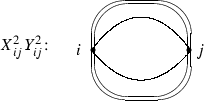
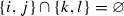
For a show of participation of variable \(X_{ij}\) in some monomials, we will use a segment (vertical or horizontal) whose ends are marked by letters i, j and also an arc with marked ends. For  we will use a thickened segment or arc.


Remark 5.2
The whole quartic form q is equal (according to [4, pp. 363–364]) to

where

G is the collection of distinct 70 four-subsets  of
of  , \(i{<}j{<}k{<}l\). The parentheses are small Pfaffians considered in Example 1.3 (a).
The total number of monomials in \(F_4\) is 1036, but it is possible to see it after a reduction of similar terms. Accurate Cooperstein’s calculations show the following description of expansion for \(F_4\):
-
(i)
There are 28 monomials
arising from \(d(X,Y)^2\), they have coefficient 1. The sum of these monomials is denoted below by the symbol \(d_1(X,Y)\).
-
(ii)
If \(i<j,k<l\),
 , then the primitive monomial
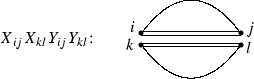
has coefficient \((-2)\) in \(F_4\). The number of monomials of such a form is 210. Their sum is denoted as
 .
. -
(iii)
Any of the primitive monomials

where \(i<j<k\) have coefficient 2. The number of monomials of such a form is 168. Notation for their sum is \(2d_3(X,Y)\).
-
(iv)
There are 210 primitive monomials of the form
$$\begin{aligned} X_{i_1j_1}X_{i_2j_2}X_{i_3j_3}X_{i_4j_4},\qquad Y_{i_1j_1}Y_{i_2j_2}Y_{i_3j_3}Y_{i_4j_4} \end{aligned}$$arising from two Pfaffians. In \(F_4\), such a primitive monomial has coefficient
 as we have seen in Example 1.3, especially in pictures from Example 1.3 (b).
 -
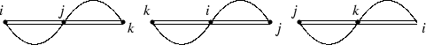
(v)
The below square circuit with four distinct vertices a, b, c, d presents a primitive monomial
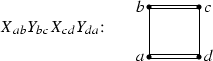
taken in \(F_4\) with coefficient \(4(-\,1)^{\sigma (abcd)}\), where \(\sigma (abcd)\) is the number of ordered pairs (p, q) with property \(p>q\) among four pairs (a, b), (b, c), (c, d), (d, a). The coefficient is invariant with respect to the circular permutations of numbers a, b, c, d or the change of their order to the inverse one.

 , then the primitive monomial
 .
.

 as we have seen in Example
A simple corollary of these pictures: the simultaneous circular permutation \( (1,2,\dots , 7,8)\) of indices of 56 variables \(X_{ij},Y_{ij}\) (and the iterations of the permutation) preserves every family (i)–(v), image of every monomial has the same coefficient as its preimage. In other words, substitution of variables induced by the permutation preserves the quartic form \(F_4\). Indeed, for types (i)–(iii) the assertion is trivial, for type (iv) it was proved at the end of Remark 1.3 (b), (1), for type (v) it is necessary to prove that
where “\(+\)” means addition modulo 8. If all the numbers are less than 8, then the congruence is obvious, if one of the numbers is 8, then one can suppose that \(d=8\), but in the last case the proof of the congruence is easy. So the linear transformation

preserves the quartic form \(F_4\), it is similar to rotation R from (1).
Definition 5.3
The quarter of sum of monomials of types (iv), (v), taken with the above signs will be denoted by the symbol D(X, Y) and we will call it Dickson’s form (see [5, pp. 66–67]).
So, the quartic form can be written as
A geometric meaning of monomials from Dickson’s form D(X, Y) is described in the following proposition.
Proposition 5.4
There exists a one-to-one correspondence between 56 variables \(X_{ij}, Y_{ij}\) and 56 exceptional curves on a non-singular Del Pezzo surface of degree 2 such that if x, y, z, w are four distinct variables and \(E_x,E_y,E_z,E_w\) are the corresponding exceptional curves, then the product xyzw has a non-zero coefficient (i.e., \(+\,1\) or \(-\,1\)) in D(X, Y) if and only if curves \(E_x,E_y,E_z,E_w\) constitute a tetrad on the surface (tetrad is a quadruple of \((-\,1)\) curves such that the intersection number of any two distinct curves equals 1).
Proof
The Del Pezzo surface S is a result of blow-up \(\mathrm{\Sigma }\) of a set of seven points \(\{P_1,P_2,\dots ,P_7\}\subset {\mathbb {P}}^2\). The exceptional curves are
-
\(L_{i}=\mathrm{\Sigma }^{-1}(P_i)\), \(i=1,\dots ,7\),
-
\(C_i\), the proper \(\mathrm{\Sigma }\)-preimage of a cubic with a double point \(P_i\) containing all other
 ,
, -
\(M_{ij}\), the proper \(\mathrm{\Sigma }\)-preimage of a line through
 ,
, -
\( Q_{ij}\), the proper \(\mathrm{\Sigma }\)-preimage of a conic containing
 .
.
 ,
, ,
, .
.The total number of enumerated curves is \(7+7+21+21=56\).
The correspondence between variables and \((-\,1)\) curves is as follows:
The tetrads are
where  ,
,

where  ,
,  ,
,
where  ,
,  . We omit illustrating pictures of quadruples (or triplets) of plane curves, where any two curves of such a set have a free (i.e., out of \(\{P_1,P_2,\dots ,P_7\}\)) point of intersection. \(\square \)
Remark 5.5
A simple corollary is existence of exactly 630 tetrads on Del Pezzo surface of degree 2. Indeed, there are 630 monomials in Dickson’s form. Further, it is clear that the proposition presents an analog of correspondence between the monomials of cubic form and tritangent planes of a non-singular cubic surface (see Remark 2.7). Moreover, the anticanonical map of Del Pezzo surface of degree 2 maps the surface onto the projective plane, it maps the 56 exceptional curves to 28 bitangents of the plane quartic curve which is the branch locus of the anticanonical map. The 630 tetrads are mapped onto 315 tetrads of bitangents of the quartic curve. These 315 tetrads are mentioned in a table from [17, no 262, p. 232], see also [17, pp. 227, 233, 387, 388] or [18, pp. 278, 285]. Salmon writes that Cayley composed the table, moreover, in the German translation, Fiedler writes in remarks (pp. 462–463) about existence of Cayley’s manuscript devoted to the bitangents. Salmon characterizes the quadruples as tetrads of bitangents such that the eight points of contact are on a conic. There is a distribution of the set of tetrads in two subsets, one subset contains 105 tetrads of type 12.34.56.78 (there is a small picture of four disjoint segments similar to our pictures for monomials of the Pfaffian), the other subset contains 210 tetrads of type 12.23.34.41 [there is a small picture of a quadrangle similar to our pictures for monomials of type (v)]. The distribution corresponds to our presentation of Dickson’s form as the sum of two subsets of monomials of types (iv), (v). There exists a more combinatorial description of these 315 tetrads of bitangents. Any bitangent with indices p, q (corresponding to  ) presents an odd theta characteristic marked (according to [2, no 205, pp. 305–306] or [17, pp. 387–388]) by a
  matrix whose entries are taken from \({\mathbb {Z}}_2\) (oddness means that the inner product of two rows equals 1 modulo 2), the sum of four odd theta characteristics for any tetrad of bitangents is equal to zero
  matrix.
It is necessary to add that the first partial derivatives of Dickson’s form contain 45 monomials, these derivatives are equivalent to the cubic form \(F_3\) (see [5]), this fact resembles some properties of determinants and Pfaffians, see Example 1.3 (d).
Definition 5.6
(Steiner sets and pairs of opposite Steiner sets) Figure 1 below shows two kinds of Steiner sets (compare a classical definition in [15, p. 354]). They are  and
and  , where

Both the classical analogs of these types are given in [15, p. 357].

(a) The upper part of \(\langle p, q\rangle \). (b) The upper part of \(\langle ijkl, rstu\rangle \).

(a) The lower part of \(\langle p, q\rangle \). (b) The lower part of \(\langle ijkl, rstu\rangle \).
More formally,

We call  and \(S(y:p,q)\) opposite, and also
  and
and  opposite. In Figs. 1 and 2, the opposite sets are disposed vertically. The above pairs of opposite Steiner systems are denoted by symbols \(\langle pq\rangle \) and
  . Certainly,

and permutations into the quadruples  do not change the corresponding pair.
The vertices of graph \(\mathrm{\Gamma }(S^*)\) of Steiner pairs are pairs of opposite Steiner systems, two pairs are connected by an edge if the symmetric difference of pairs considered as sets of variables is again a set of variables belonging to a pair of opposite Steiner systems. The symmetric difference is a partial operation on the set of vertices of the graph.
We will compare this graph with the graph \(\mathrm{\Gamma } (E_7)\) having a partial operation on the set of its vertices, the operation is defined in Example 1.3 (f) for any semisimple group. Note that \(W(E_7)\) acts naturally on \(\mathrm{\Gamma } (E_7)\).
Remark 5.7
There are 63 pairs of opposite Steiner sets, 28 pairs of type \(\langle pq\rangle \) and 35 pairs of type  . The number 63 coincides with the number of projective roots for the exceptional group \(E_7\), this coincidence is not occasional as we will see below.
Theorem 5.8
There exists an isomorphism between graphs \(\mathrm{\Gamma } (E_7)\) and \(\mathrm{\Gamma }(S^*)\). Moreover, there exists an action of \(W(E_7)\) on \(\mathrm{\Gamma }(S^*)\) such that the isomorphism is \(W(E_7)\)-equivariant.
Proof
There are three types of pairs of adjacent vertices in \(\mathrm{\Gamma }(S^*)\). The first type consists of vertices \((\langle pq\rangle ,\langle qr\rangle )\), \(r\ne p\), \(r\ne q \), other pairs of adjacent vertices are ( ), where
  ,
,  , the third kind of adjacency is (
 ). The symmetric differences of such adjacent vertices are

The subgraph of \(\mathrm{\Gamma }(S^*)\) generated by following seven pairs of opposite Steiner systems:

is

and it coincides with Dynkin diagram for \(E_7\). One can map \(e_1,\dots ,e_7\) to basic projective roots of \(E_7\) connected by such a diagram. All other 56 double sixes are expressible via the basic \(e_1,\dots ,e_7\) with the help of symmetric difference. These expressions are parallel to presentations of non-basic projective roots with the help of partial addition. The rest of the proof goes as the proof of Theorem 2.12. We omit this part.\(\square \)
Remark 5.9
This remark is similar to Remark 2.13. We describe explicitly the action of \(W(E_7)\) (more precisely, actions of some representative of this group in the normalizer of a maximal torus) on  .
.
We consider the group of linear transformations preserving projectively the quartic form \(F_4\) and its toric subgroup \({\mathbb {T}}\) consisting of linear substitutions expressible as multiplications of variables from the set  of 56 variables by non-zero constants. Any element of such a torus is completely determined by the action of the element on seven variables
(here we use simultaneously old and new variables). Let us take six non-zero numbers \(\lambda _i\in K^*\), \(i=1,\dots ,6\), and a number \(\mu \in K^*\). Let \(\theta \in K^*\) be defined as in Remarks 2.13, 2.14, that is  . If one uses notations from Definitions 4.1, 4.2, then the toric action on Z(A) is defined by

where \({\Lambda } \) is taken from Remark 2.14, it preserves q (and \(F_4\) after a change of variables). So we have defined a maximal (7-dimensional) torus \({\mathbb {T}}\) in the group of projective transformations preserving the quartic form. Let \({\mathbb {N}}\) be the normalizer of \({\mathbb {T}}\) in the group of linear transformations preserving projectively \(F_4\). As well as in Remark 2.13, here we will use the sign changing subgroup \(S{\mathbb {T}}\) of \({\mathbb {T}}\) consisting of the above elements with \(\mu , \lambda _i\in \{+\,1,-\,1\}\), and the sign changing subgroup \(S{\mathbb {N}}\) of the normalizer \({\mathbb {N}}\).

\(S{\mathbb {T}}\) is an invariant subgroup of \(S{\mathbb {N}},S{\mathbb {T}}\) is an elementary abelian 2-group isomorphic to \({\mathbb {Z}}_2^7\). It is possible to generate \(S{\mathbb {N}}\) by some involutive (modulo the torus) elements corresponding to Steiner pairs.
Every Steiner pair s determines a transformation  such that \(T_{s}\) preserves the set of variables from s (up to signs of variables), interchanges Steiner pairs (more precisely, the sets of its variables taken up to sign),
  , \(T_{sp}^4=1\).
Explicit description of \(T_{s}\) is as follows. By use of notations from Definitions 4.2, 4.1, the transformation \(T_{\langle 78\rangle }\) is defined by

that is up to signs in the upper row, it coincides with reflection \({\texttt {R}}\).
Transformations \(T_{\langle pq\rangle }\), where \(1\leqslant p<q\leqslant 6\), are contragredient extensions of corresponding transformations from Remark 2.13. If \(T_s\) is a transformation from this Remark, \({\widetilde{T_s}}\) is its conragradient transformation (see the proof of Theorem 4.3 and [20, p. 180]), \(\theta _s\) is the norm multiplicator of \(T_s\), i.e.,
then the extended transformation for \(T_s\) is
If s is a double six \(\langle pq\rangle \) where \(1\leqslant p< q\leqslant 6\), then for the Steiner pair s marked by the same symbol \(\langle pq\rangle \), the transformation \(T_{\langle pq\rangle }\) is the contragrediently extended transformation for the double six.
The transformation \(T_{\langle i7\rangle }\) (or \(T_{\langle i8\rangle }\)) may be produced by a sequence of conjugations by rotation R mentioned in the final lines of Remark 5.2 [see formula (7)].
What is left is to describe transformations  . They are extended bifid transformations.
Below an action of the extended bifid transformation \(g=T_{\langle 1234\vert 5678\rangle }\) on the variables is described. Latin bifidus means double-sided, Fiedler used zweiseitig instead of bifid. In the situation of 28 bitangents, ordinary bifid transformations were described by Salmon (with a reference to Cayley), see [17, no 261, p. 232] or [18, no 262, p. 264]. As well as in explications by Salmon and Cayley, we take a special natural order  of eight numbers in our consideration of
  . The classics hoped that their explications of this special case are sufficiently general, but for our case it is necessary to say that a composition of analogs of three below
  matrices with sign entries for every
  case is not a simple task, bifid transformations associated with other
  can be produced by sequential conjugations of the
  sample by transformations of the form \(T_{\langle ab\rangle }\) associated with Steiner \(\langle ab\rangle \) pairs.
If  ,
,  , then \(g^*(X_{ij})=\gamma _{ij}X_{ij}\), \(g^*(Y_{ij})=\gamma _{ij}Y_{ij}\), where \(\gamma _{ij}\in \{-\,1,+\,1 \}\), the signs of \(\gamma _{ij}\) are given in the matrix below
If  , \(i\ne j\),
  , then \(g^*(X_{ij})=\epsilon _{ij}Y_{IJ}\),
  , similarly, if
  , \(i\ne j\),
  , then \(g^*(X_{ij})=\delta _{ij}Y_{IJ}\),
  , where \(\epsilon _{ij}, \delta _{ij}\in \{-1,+1 \}\), the signs of \(\epsilon _{ij}\), \(\delta _{ij}\) are given in the matrices below
More explicitely,

We omit verifications of Weyl-group properties of the transformations marked by the Steiner pairs, that is
-
involutiveness modulo the subgroup \(S{\mathbb {T}}\) of the above transformations,
-
involutiveness modulo \(S{\mathbb {T}}\) of products of two transformations associated with Steiner pairs not adjacent in \(\mathrm{\Gamma }(S^*)\),
-
the third order modulo \(S{\mathbb {T}}\) of products of two transformations corresponding to Steiner pairs adjacent in \(\mathrm{\Gamma }(S^*)\).
So we see that  . The above transformations \(T_{s}\) act on the set of Steiner pairs, these transformations preserve the structure of the graph \(\mathrm{\Gamma }(S^*)\), actions of \(W(E_7)\) on the set of projective roots of \(E_7\) and on the set of Steiner pairs are bilaterally matched.
Proposition 5.10
Brown’s cubic transformation defined in Definition 4.4 normalizes the maximal torus.
Proof
It follows from immediate verification using explicit formulas for the action of torus (they are presented in Remarks 5.9, 2.14) and formulas for the cubic transformation from Definition 4.4. More precisely, if \({\Lambda }\in {\mathbb {T}}\) is a toric element (see Remark 2.14), whose action is described is Remark 5.9, \(\nabla \) is Brown’s transformation, then it is obvious that \( \nabla {\Lambda }={\Lambda }^{-1}\nabla \).\(\square \)
Remark 5.11
The cubic transformation taken together with involutions described in Remark 5.9 generate a subgroup \({\widetilde{\mathbb {N}}}\) in the group of automorphisms of the affine set, the quotient group \({\widetilde{\mathbb {N}}}/{\mathbb {T}}\) can be considered as an extended Weyl group.
References
Arzhantsev, I., Flenner, H., Kaliman, S., Kutzschebauch, F., Zaidenberg, M.: Flexible varieties and automorphism groups. Duke Math. J. 162(4), 767–823 (2013)
Baker, H.F.: Abel’s Theorem and the Allied Theory. Cambridge University Press, Cambridge (1897)
Brown, R.B.: Groups of type \(E_7\). J. Reine Angew. Math. 236, 79–102 (1969)
Cooperstein, B.N.: The fifty-six-dimensional module for \(E_7\): I. A four form for \(E_7\). J. Algebra 173(2), 361–389 (1995)
Dickson, L.E.: The configurations of the 27 lines on a cubic surface and the 28 bitangents to a quartic curve. Bull. Amer. Math. Soc. 8(2), 63–70 (1901)
Freudenthal, H.: Oktaven. Ausnahmegruppen und Oktavengeometrie. Mathematisch Instituut der Rijksuniversiteit te Utrecht, Utrecht (1951)
Freudenthal, H.: Oktaven, Ausnahmegruppen und Oktavengeometrie. In: Springer, T.A., van Dalen, D. (eds.) Hans Freudenthal Selecta, pp. 214–269. European Mathematical Society (EMS), Zürich (2009)
Freudenthal, H.: Oktaven, Ausnahmegruppen und Oktavengeometrie (an extended Russian translation by B.A. Rosenfeld). Matematika 1(1), 117–153 (1957)
Freudenthal, H.: Zur ebenen Oktavengeometrie. Nederl. Akad. Wetensch. Proc. Ser. A 56, 195–200 (1953)
Freudenthal, H.: Zur ebenen Oktavengeometrie. In: Springer, T.A., van Dalen, D. (eds.) Hans Freudenthal Selecta, pp. 288–293. European Mathematical Society (EMS), Zürich (2009)
Henderson, A.: The Twenty-Seven Lines Upon the Cubic Surface. Ph.D. Thesis, University of Chicago (1915)
Jacobson, N.: Structure and Representations of Jordan Algebras. American Mathematical Society Colloquium Publications, vol. 39. American Mathematical Society, Providence (1968)
Jordan, C.: Traité des Substitutions Algébriques. Gauthier-Villars, Paris (1870)
Manin, Yu.I.: Cubic Forms. Nauka, Moscow (1972); English translation by M. Hazewinlel, North-Holland Mathematical Library, vol. 4. North-Holland, Amsterdam (1986)
Miller, G.A., Blichfeldt, H.F., Dickson, L.E.: Theory and Applications of Finite Groups. Wiley, New York (1916)
McCrimmon, K.: A Taste of Jordan Algebras. Universitext. Springer, New York (2004)
Salmon, G.: A Treatise on the Higher Plane Curves, 3rd edn. Hodges, Foster, Dublin (1879)
Salmon, G.: Analytische Geometrie der Höheren ebenen Curven (German translation by W. Fiedler). Teubner, Leipzig (1873)
Shafarevich, I.R.: On some infinite-dimensional groups. II. Math. USSR-Izv. 18(1), 185–194 (1982)
Springer, T.A., Veldkamp, F.D.: Octonions, Jordan Algebras and Exceptional Groups. Springer Monographs in Mathematics. Springer, Berlin (2000)
Acknowledgements
First of all the author would like to express his gratitude to Ernest Vinberg, who attracted the attention of listeners to the subject during his lectures at the Moscow conference “Lie algebras, Algebraic Groups and Theory of Invariants” (January 30–February 4, 2017). His lecture from February, 4 was devoted to exceptional groups and the cubic form \(F_3\). The author also wishes to thank Ivan Cheltsov who encouraged to contribute to the collection dedicated to William Edge. The author is truly grateful to an anonymous referee for his/her efforts, remarks and comments.
Author information
Authors and Affiliations
Corresponding author
Additional information
In memory of William Edge
Appendix: Matrix \({\mathbb {M}}(F_3)\)
Appendix: Matrix \({\mathbb {M}}(F_3)\)

Rights and permissions
About this article

Cite this article
Gizatullin, M. Two examples of affine homogeneous varieties. European Journal of Mathematics 4, 1035–1064 (2018). https://doi.org/10.1007/s40879-018-0228-y
Received:
Revised:
Accepted:
Published:
Issue Date:
DOI: https://doi.org/10.1007/s40879-018-0228-y