Traffic Anomaly Detection Model Using K-Means and Active Learning Method

Abstract

As the digital world becomes the main complement to the physical world, establishing a solid line of defense against cyber attacks becomes critical and arduous. The intrusion detection systems (IDSs) based on the supervised learning method have achieved excellent performance, which requires a large amount of labeled data in the training phase. However, attacks occur much less frequently than normal behaviors, and it is difficult to obtain accurate labels. In addition, IDSs based on supervised learning cannot identify unknown attacks. At the same time, the problem that detection accuracy varies greatly with different applications is very significant in traditional unsupervised learning methods. Therefore, it is necessary to perform high-precision anomaly detection on unlabeled samples. This paper proposes a traffic anomaly detection model using K-means and Active Learning Method (ALM), which is mainly composed of a feature extraction module and an anomaly detection module. Firstly, the Pearson correlation coefficient and Light Gradient Boosting Machine (LightGBM) are used in the feature extraction module to select important features. Secondly, K-means divides the characteristic-processed traffic into normal or abnormal categories. Finally, the results of K-means are diffused through ALM, and new classification results are obtained after defuzzification, thereby improving the accuracy of anomaly detection. The latest CICDDoS2019 data set is used in the experiment. Experimental results show that the detection accuracy of the proposed model is above 90%, and the F1 score is above 95%, regardless of whether it is a binary classification of a single attack or a mixed classification of multiple attacks. Compared with three unsupervised learning methods K-means, Auto-encoder and short-term memory (LSTM) and three supervised learning methods Naive Bayes (NB), Support Vector Machine (SVM), Decision Tree (DT), the proposed model has higher classification accuracy and better generalization effect. This article is very helpful for exploring the application of unsupervised learning methods in network intrusion detection systems based on the characteristics of the data itself.

1 Introduction

Network applications and smart devices occupy people's daily lives, accompanied by a large amount of Internet access. With the continuous development of information technology, cyber attacks have become more variable and unpredictable. Therefore, network anomaly detection has aroused great interest of researchers. Some intrusion detection systems are specifically designed to identify attacks and issue alerts [1, 2]. However, there are still many problems in the complex network environment. For decades, supervised learning based on machine learning is one of the most popular methods, which requires a large number of labeled samples to train the model. However, the cost of obtaining explicit tags is high, which requires manual tagging by network experts. In addition, it is difficult for a model trained with labeled data to recognize new attacks before they appear, which requires the detection model to be sensitive enough to detect unknown attacks. Therefore, there is an urgent need for a detection system that does not require labeled data. In order to break through this limitation, this paper adopts the method of unsupervised learning.

There are three main anomaly detection methods: supervised learning method, semi-supervised learning method and unsupervised learning method [3]. As a general rule, data needs to be pre-labeled in pre-training for supervised and semi-supervised learning methods [4, 5]. At the same time, with the advantage of automatic learning from network traffic and allowing for bypassing heavy learning, unsupervised learning methods have become an important area[6]. In recent studies, the number of applications of machine learning (ML) and artificial intelligence (AI) technologies that have achieved excellent performance and versatility has greatly increased [7, 8]. However, most of this type of research focuses on supervised learning. In addition, ML and AL methods have always relied on feature engineering sets based on human analysis, which requires time-consuming and laborious professional analysis.

Generally speaking, among unsupervised learning methods, K-means is more popular than other unsupervised methods and provides more insights about complex data. One of the reasons is the implicit assumption of K-means, that is, abnormal samples are far fewer than normal samples [1], which is largely consistent with the actual situation of network traffic. Another reason is that K-means can handle noisy, incomplete and sampled data. In addition, the number of parameters involved in K-means is limited, and there is no need to spend a lot of effort to adjust the parameters. However, for different applications and data types, its performance will vary greatly. In order to overcome this problem, a fuzzy theory was chosen, that is, an Active Learning Method (ALM) to optimize the results of K-means. Fuzzy theory takes into account the uncertainty of data and classification in clustering, and is more suitable for situations where there is no clear boundary for clustering in practical applications. In addition, the ALM will consider the density and shape of the data, and blur the results of K-means, thereby bringing more accurate classification and reducing noise or outliers. In this way, abnormality detection can be performed well.

The contributions of this paper can be summarized as follows:

• (1) A network anomaly detection model using K-means and ALM is proposed, and ALM is applied to the field of network traffic with large feature dimensions and large data volume. This model not only can obtain good detection performance under a single attack type, but also can obtain good detection performance in anomaly detection scenarios with multiple mixed attack types.

• (2) Through ALM, starting from the data itself, considering the density and shape of the application data, a more natural degree of membership can be obtained, and thus better detection results can be obtained. It improves the detection results obtained using the K-means method on the CICDDoS2019 data set, and achieves better performance in accuracy, recall and F1 scores.

• (3) Enhancing the ability to eliminate noise and outliers through ALM, which will interfere with the classification process and lead to poor detection accuracy.

The rest of this article is structured as follows. Some related work is arranged in Sect. 2. In Sect. 3, we introduce the basic background of ALM, which is necessary for our work. Section 4 describes the specific steps and principles of the proposed model. In Sect. 5, the advantages of this method are verified through experiments. Finally, conclusions are provided in Sect. 6.

2 Related Works

As we all know, with the rapid development of information technology, network intrusion detection is playing an increasingly important role in network security [9]. In particular, network traffic analysis will seriously affect the detection of certain abnormal behaviors. This is mainly because network traffic records the entire network behavior and contains a lot of information [10]. It is widely accepted that the first step in anomaly detection is to extract valid information and valid features from the source data, which will affect the time of traffic behavior detection and the accuracy of anomaly detection [11]. Similarly, this paper uses Pearson correlation coefficient and Light Gradient Boosting Machine (LightGBM) to perform feature selection, and selects the most concise non-redundant feature subset for subsequent anomaly detection.

In recent decades, there have been many network anomaly detection systems based on supervised [3, 12,13,14,15] and semi-supervised [16] learning methods. Support Vector Machine (SVM) is a supervised learning method worth mentioning, which can detect and process large data in real time [12]. Due to the popularity of distributed systems, the anomaly detection system is no longer limited to a single SVM. Jun et al. used the gradient descent algorithm with Spark to train the SVM classifier to improve the speed of model training [13]. Another excellent supervised learning technique is Naive Bayes (NB), which has a basic assumption that the conditional independence of data features, which is usually not the case for intrusion detection data features [3]. And Panda et al.[14] achieved 96.5% accuracy in the two-classified data set through the NB classifier. In addition, it has recently become popular to combine ML and AI methods with traditional supervision methods. The research by Kazi et al. [15] proposed an artificial neural network (ANN) based on machine learning to perform wrapper-based feature selection first, and it showed an accuracy of 94.02%. Yin et al. [16] proposed a recurrent neural network (RNN-IDS) for intrusion detection is proposed and compared it with machine learning methods such as J48, ANN, random forest, and SVM. Experimental results showed that RNN-IDS was superior to traditional machine learning classification methods in terms of two-class and multi-class performance. The literature [17] proposed a new method of intrusion detection based on semantic recoding and deep learning, namely SRDLM, by analyzing and recoding the differences of abnormal traffic in multiple semantic dimensions. Compared with traditional ML methods, its average performance was improved by more than 8%.

The typical technique used in the semi-supervised learning method is only to build a model for the category corresponding to the normal sample, and use the model to identify the attack. It usually applies detection in scenarios where there is no historical accident or attack data [18]. In [19], four ML models were used for detection, which were feedforward neural networks, autoencoders, deep belief networks, and long and short-term memory networks; it includes supervised and semi-supervised ML methods. The results showed that the classification effect of the deep feedforward neural network was significant, and the detection rate was higher than that of the autoencoder and the deep belief network.

However, all of these methods mentioned above require labeling data, which is expensive, because the corresponding professionals must carefully check the traffic data and determine whether the specific pattern is an attack or a normal sample [20]. Likewise, none of them provide effective solutions for identifying new abnormal behaviors. This is why there is an increasing demand for network intrusion detection systems (NIDSs) based on unsupervised learning.

Choi et al. [20] used an unsupervised learning algorithm auto-encoder to monitor and analyze network traffic, and its accuracy was better than previous cluster analysis algorithms that reached 80% accuracy. Vartouni et al. [21] applied unsupervised machine learning algorithms based on anomaly detection in these Web application firewalls to protect servers from HTTP traffic. It used a deep neural network, namely Stacked Auto-Encoder, for feature learning, and then used an isolation forest as a classifier. In order to detect abnormal traffic in Web applications and extract advanced features from massive data, Moradi et al. [22] combined deep neural networks and parallel feature fusion. Among them, stacked autoencoders and deep belief networks were used for feature extraction and learning, and a SVM, isolation forest, and elliptical envelope were used as subsequent classifiers. The literature [23] proposed a long short-term memory (LSTM)-Gauss-Nbayes method for outlier detection in industrial Internet of Things. It used long and short-term memory neural networks to build models on normal time series, and then applied Gaussian Naive Bayes models to make false predictions and used them to detect outliers. It took the advantages of LSTM and Gaussian Naive Bayes model, and had high detection accuracy.

In fact, most of these unsupervised machine learning solutions are aimed at specific problems and may be difficult to promote, and their generalization ability is not strong. In the work by Syarif et al. [24], a NIDS based on cluster analysis was developed. They studied the performance of various clustering algorithms, such as K-means [25], K-medoids [26], expectation–maximization(EM) clustering [27], and distance-based outlier detection [28]. The results showed that the distance-based outlier detection algorithm was better than other algorithms with an accuracy of 80.15%, while the model based on the supervised learning algorithm shows high performance, with an accuracy of about 90% [19]. Syarif et al. hypothesized that abnormal behaviors are far less than normal behaviors, which was largely consistent with the actual situation of network traffic. However, their method does not consider how to set the threshold to distinguish between normal and abnormal. Therefore, fuzzy theory has been widely used in unsupervised methods [29,30,31], which was first proposed by Zadeh [32]. It gave a better division method than the hard boundary, and used the degree of membership to indicate the degree to which a point belongs to a certain class, which was more in line with the actual situation.

Considering that the normal and suspicious behaviors of computer networks were difficult to determine, because the boundaries between them cannot be well-defined, fuzzy rough C-means were applied to cluster analysis in [29]. The model combined fuzzy set theory and rough set theory to detect network intrusions, with an accuracy rate of 82.46%. Sharma et al. [30] proposed an intrusion detection system based on density maximization of fuzzy C-means clustering to improve clustering efficiency. In addition, Hamamoto et al. [31] put forward a network anomaly detection system combining genetic algorithm and fuzzy logic, with an accuracy rate of 96.53%. Previous studies have generally confirmed that fuzzy theory significantly improves the performance of a single algorithm. Based on the theory of fuzzification theory and unsupervised learning, this paper proposes a network anomaly detection model using K-means combined with ALM, where SALM is a fuzzy theory.

3 Active Learning Method

This section will briefly introduce the basic concepts of ALM employed in our proposed model. A more detailed description can be found in [33,34,35]. The ALM theory was first proposed by Saeed Bagheri Shouraki et al. and was implemented in hardware[36]. This idea comes from the human brain. Humans have an excellent ability to easily process complex information. Where the most prominent norm of the brain is to extract and use pure qualitative knowledge, a true soft computing method is needed to approach the true brain capabilities[37]. It defines the information obtained from the outside world as multiple single-input single-output systems, then extracts and saves knowledge by fuzzing the input information, and finally combines multiple systems to form an inference system, as shown in Fig. 1. Later, in the literature [38], ALM is expressed in mathematics and precise expressions. First, project the data onto multiple X–Y axis planes, and each plane is defined as a subsystem. Secondly, assuming that each subsystem is a single-input single-output system, then each plane will get a key curve, which describes the change curve of the output value Y with the input value X. Considering the actual process of human brain processing information, there will be a fuzzification process before the key curve is obtained, and the whole process is executed by the Ink-drop-spread (IDS) unit [39]. Finally, all the subsystems are combined, and the key curves are weighted and combined to obtain an inference system and a set of inference rules, and then make predictions.

Fig. 1

ALM breaks a Multiple-Inputs-Single-Output (MISO) system into several Single–Input–Single–Output (SISO) subsystems. Each SISO subsystem is then model by an IDS plane. Then an inference engine aggregates the behavior of the subsystems to obtain the final output[43]

The IDS Unit is a two-dimensional data plane, which extracts two types of information, Narrow path and Spread, as shown in Fig. 2. The Narrow path describes how the output varies with the input features and the Spread shows the importance and the effectiveness of this IDS Unit [39].

Fig. 2

Narrow path and spread of an IDS plane [41]

In each IDS unit, a three-dimensional fuzzy membership function (called ink drop) is applied to each data point as the diffusion information in each plane. Subsequently, all the diffusion information generated at each point is aggregated to generate a smooth pattern, thereby enhancing the impact of each data point. It is generally believed that each data not only affects its exact point, but also affects neighboring points, but it has a low degree of confidence ^[2]. Let $d(x,y)$ represent the darkness at the IDS plane coordinate. The ink drop point $p({x}_{i},{y}_{i})$ related to data diffusion can be expressed as Eq. (1):

$$\Delta d\left( {x_{i} + m,y_{i} + n} \right){\text{ }} = f\left( {m,n} \right), - Ir \le m,n \le Ir,$$

(1)

where $\Delta d$ represents the change in darkness at coordinates $\left({x}_{i}+m, {y}_{i}+n\right)$. $Ir$ and $f$ are applied to describe the shape of the ink drop, which denotes the radius and function of the ink drop, respectively. The function $f$ can be a Gaussian or any convex function and it has a characteristic that the amplitude decreases as it moves away from the center [40].

The formula for extracting the Narrow path is described in Eq. (2) [41].

$$\varphi \left(x\right)=\left\{t\in Y\right| \sum_{y= {y}_{\mathrm{min}}}^{t}d\left(x,y\right)\approx \sum_{y=t}^{y= {y}_{\mathrm{max}}}d\left(x,y\right)\},$$

(2)

where ${y}_{\mathrm{max}}= \underset{y\in Y}{\mathrm{max}}y.$

After performing diffusion processing on each two-dimensional data plane, use the fuzzy inference system to integrate them to form a set of inference rules, and finally make predictions. Figure 3 describes the inference process in which the Narrow path and Spread values are used for fuzzy inference to generate a rule set. The combination of each IDS Unit is showed in Eq. (3), and ${\beta }_{ik}$ represents the confidence of the Narrow path ${\varphi }_{ik}.$

Fig. 3

Structure of 2-input 1-output ALM [43]

$$\begin{array}{c}y\left(x\right)={\beta }_{i1} {\varphi }_{11}+\dots +{\beta }_{ik}{\varphi }_{ik}+\dots +{\beta }_{n{l}_{n}}{\varphi }_{n{l}_{n}.}\end{array}$$

(3)

The ALM method has achieved good results in previous applications, but considering that when the human brain processes information, each subsystem is not independent, and the characteristic information will affect each other. It is more suitable for the actual situation to regard all the characteristic information as a whole. Javadian [42] initially combined the ALM algorithm with the DBSCAN clustering method in 2017. In reference [43], he no longer regards each input feature and output as a single-input single-output subsystem, but a system containing all the features. Therefore, in his rule, there is no step of combining N subsystems formed by N features into an inference system. He transformed it into building a system with N-dimensional features; at the same time, the membership function of the diffusion in the IDS unit also became N-dimensional. This kind of rule is better because only one feature was considered before, and mutual influence was not considered. And it takes time to determine the weights in the inference system. He confirmed in the literature [43] that this change of the fuzzification process in the inference process also achieved good results, as shown in Fig. 4. Figure 4a is the result of K-means clustering algorithm. It did not cluster the data set correctly, nor did it detect noise and outliers. Figure 4b is the result of fuzzification of K-means results using ALM. It can be seen that the ALM algorithm can correct the data points of wrong clustering and detect the abnormal points and noisy data points at the same time. Figure 4c and d show the results of Fuzzy C-means (FCM) and the Possibilistic C-means (PCM) algorithms, respectively. Both algorithms allocate some points from the right cluster to the left cluster, and vice versa. They also have problems detecting noise and outliers. FCM’s "sum of membership equals one" rule leads to false noise detection. Unlike ALM considering the shape and density of clusters to assign membership degrees, FCM and PCM use the distance function from the cluster center as the membership function.

Fig. 4

An example to demonstrate above three claims [43]

But in the experiment done by Javadian, the feature dimension is not very large, and the data set is relatively small. This article also adopted the same idea as him, and applied it to a network traffic data set with a large amount of data and a larger feature dimension. And before use, the features are processed in more detail to make it a more suitable model. The ALM algorithm is a fuzzy algorithm, which assumes that an object can belong to different sets but have different degrees of membership. But in traditional theories, the attribution of an object has a clear boundary, and it either belongs to or does not belong to a unique category. Due to the robustness of fuzzy sets, they are widely used in clustering. In many practical situations, fuzzy clustering is more natural than hard clustering. Because it considers the uncertainty of data and clusters, it is more suitable for practical applications, where there is no clear boundary between clusters. In fact, the ALM algorithm is a post-processing of the results of the clustering algorithm, through which we can make good use of the advantages of both the clustering algorithm and the fuzzy clustering. The ALM makes up for the shortcomings of clustering algorithm that only determines the degree of membership based on the distance from the center point. Considering that all data points in a cluster have an impact on the membership degree of each precise point in the cluster, ALM assigns membership degrees to each data object according to the shape of the cluster, the number of data in the cluster, and the density distribution of the cluster. It takes into account the characteristics of the data itself, and improves the prediction accuracy from the data processing.

The application of ALM in clustering has three advantages:

• (1) Obtaining a more natural membership degree. The obtained membership matrix is based on the shape and density of each data point, rather than simply based on the distance from the center point, which is the main advantage of the ALM.

• (2) Improving the quality of clustering. As a post-processing of the clustering algorithm, the ALM improves the quality of the clustering results in most cases.

• (3) Ability to eliminate noise and outliers. The ALM algorithm itself has this function, and some clustering algorithms have the problems of noise and outlier data points, but the ALM algorithm can reduce the impact of these data points, because the factors considered by ALM are not limited to distance.

4 Model and Methods

4.1 Anomaly Detection Framework

This model is dedicated to attaching a superior detection result with a small amount of labeled data. In order to complete the experimental demonstration and explanation, the whole process is divided into two stages. As show in Fig. 5, there are Feature Extraction module and Anomaly Detection module.

Fig. 5

Intrusion Detection System combining K-means and ALM

The Feature Extraction Module aims to convert the original data into a matrix and seek for significant feature spaces. Considering that the quality of feature selection directly affects the effect of network traffic abnormality determination, it is essential to find an effective feature set, but it should not be too large, which will cause the detection time to be too long. In addition, there are some unsuitable data in the original data that cannot be processed by the K-means method, and they will also be processed in this module. Then, the main anomaly detection process of our model begins.

The anomaly detection module mainly includes K-means, Fuzzy modeling and Defuzzification process. The features output by the Feature Extraction process will be sent to K-means for basic division. The pre-processed traffic will be divided into two classes, namely normal traffic and abnormal traffic. Subsequently, each data of each cluster will be fuzzified by Fuzzy modeling. Finally, defuzzification is used to obtain a detection result that is different from the K-means stage.

It is worth mentioning that, referring to Javadian, considering the mutual influence of various features and detection efficiency, the ALM algorithm in this article uses N-dimensional membership functions for diffusion, and then removes the step of establishing inference rules. Only the IDS idea in the ALM algorithm is used to perform Fuzzy modeling, which is mainly used to fuzzify the cluster. Ink Drop Spread assumes that each data point has a fuzzy membership function for points other than itself, which is defined as an “ink drop”. Then all the ink drops of the same data point are overlapped and normalized to obtain the points of the membership degree of the data belonging to the cluster, so as to achieve the fuzzy effect.

4.2 Feature Extraction

At this stage, the filter method and embedded method are combined for feature extraction. The filter method scores various features based on correlation analysis, and then sets a threshold to select features. This article chooses to analyze the variance of the features themselves and the correlation between the features. The former has a threshold of 0 and the latter has a threshold of 0.65. The embedded method selects several features or excludes several features at a time according to the objective function (usually the prediction effect score). In this article, the training is mainly carried out by LightGBM. The detailed steps are given below. The whole data preprocessing is divided into four steps. Through these four steps, a feature set with the largest amount of information but sufficiently concise can be obtained.

Step 1:

Single feature analysis. This step mainly removes the features with variance 0. Common sense implies that the smaller the variance of the data, the more stable the feature distribution. Not to mention that the variance of a feature is close to 0. This means that the value of this feature is almost the same for normal flow and abnormal flow, which shows that this feature is not helpful for distinguishing abnormalities.

$$\begin{array}{c}variance=\frac{\sum_{i=1}^{n}{\left({X}_{i}-\overline{X }\right)}^{2}}{n} .\end{array}$$

(4)

Step 2:

Correlation analysis of characteristics. In step 1, the variance of a single feature is analyzed, and then in this step, the relationship between the features is explored through the Pearson correlation coefficient. It measures the strength and direction of the linear relationship between two variables X and Y, which can be define as

$$\begin{array}{c}{\rho }_{X,Y}=\frac{\sum (X-\overline{X })(Y-\overline{Y })}{\sqrt{\sum {(X-\overline{X })}^{2}{(Y-\overline{Y })}^{2}}},\end{array}$$

(5)

where $\overline{X }= \frac{1}{T}\sum_{t=1}^{T}{X}_{t}$ and $\overline{Y }= \frac{1}{T}\sum_{t=1}^{T}{Y}_{t}$.

The value of ${\rho }_{X,Y}$ is between − 1 and 1. When the value of $X$ increases (decreases), the value of $Y$ decreases (increases), which shows that the two vectors of $X$ and $Y$ are negatively correlated. In this case, and the value of ${\rho }_{X,Y}$ is between -1.0 and 0.0. On the contrary, when the value of Y increases(decreases) as the value of X increases(decreases), the value of ${\rho }_{X,Y}$ is between 0 and 1.0.

After analyzing the correlation between every two features, a matrix can be obtained, as shown in the Eq. (6). This matrix only represents the case where there are only four features A, B, C, and D. In this article, redundant features with correlation coefficients above 0.65 are deleted, considering that they have a strong correlation with another feature.

$$\begin{array}{c}M=\left[\begin{array}{cccc}{\rho }_{\mathrm{A},\mathrm{A}}& {\rho }_{\mathrm{A},\mathrm{B}}& {\rho }_{\mathrm{A},\mathrm{C}}& {\rho }_{\mathrm{A},\mathrm{D}}\\ {\rho }_{\mathrm{B},\mathrm{A}}& {\rho }_{\mathrm{B},\mathrm{B}}& {\rho }_{\mathrm{B},\mathrm{C}}& {\rho }_{\mathrm{B},\mathrm{D}}\\ {\rho }_{\mathrm{C},\mathrm{A}}& {\rho }_{\mathrm{C},\mathrm{B}}& {\rho }_{\mathrm{C},\mathrm{C}}& {\rho }_{\mathrm{C},\mathrm{D}}\\ {\rho }_{\mathrm{DA}}& {\rho }_{\mathrm{D},\mathrm{B}}& {\rho }_{\mathrm{D},\mathrm{C}}& {\rho }_{\mathrm{D},\mathrm{D}}\end{array}\right].\end{array}$$

(6)

Step 3:

Feature importance analysis. After the first two steps of processing, only some redundant features are removed from the feature set. In order to improve the efficiency of anomaly detection, we consider using the embedding method to filter the features again, but this requires analyzing the relationship between the label and the feature to proceed. In this article, this step is used as a post-processing. This step analyzes the relationship between features and labels only after the labels have been obtained through multiple rounds of training, so as to save the feature set with the most information to improve the detection efficiency. In this step, the LightGBM is used to obtain the feature importance. LightGBM is a distributed gradient boosting framework based on decision tree algorithm. In a single decision tree model, this process is actually looking for a certain feature as a suitable segmentation point during the model building process. Then, the number of times that the feature is selected as a segmentation feature can be used as an indicator of the importance of the feature. Similarly, the importance of a feature in LightGBM is sorted according to the number of times it is used as a partition attribute in all trees. After the importance score between each feature and the label is obtained, the feature with a score of 0 is deleted.

Step 4:

Feature coding. This step mainly deals with data in a special format, because some data in a special format cannot be run in K-means. First, map non-numeric features to numeric data, including the last label column. Then, there are infinite values in some columns, and replace them with the average value corresponding to the column.

After the above four steps of processing, the original data can be reduced in dimensionality, which greatly reduces the number of features. At the same time, the amount of data are greatly reduced with the reduction of features. Therefore, this not only guarantees the validity of the data, but also improves the speed and efficiency of detection.

4.3 Anomaly Detection

After extracting the information behavior characteristics of different network flows, it is necessary to use powerful methods to perform the actual detection process.

In this module, K-means is used to divide the feature-processed data into two categories. Then in the Fuzzy modeling stage, the IDS idea in ALM is used to fuzzify each data in the category, and the membership degree of each data point belonging to each category is obtained. After defuzzification, a classification result different from K-means is obtained, and the detection accuracy is also improved.

In the process of Fuzzy modeling, it is necessary to select a function that satisfies the rule that the farther from the center point, the smaller the value of the function. This paper selects Gaussian functions that meet the above rules, as shown in Fig. 6. The steps of anomaly detection are shown in Fig. 7. Specific steps are as follows. At the same time, the Flame data set is used as a test sample to show the effect of certain steps.

Fig. 6

An ink drop pattern with pyramid shape

Fig. 7

The flowchart of anomaly detection

Step 1: Clustering:

The first step is to use the K-means algorithm for clustering, and the number of clustering categories is designated as 2, namely, normal traffic flow and abnormal traffic flow. As shown in Fig. 8, using K-means to divide Flame data into two categories: red dots and blue dots.

Fig. 8

The classification result of the Flame data set using the K-means

Step 2: Scaling:

Considering that the value range of various characteristics of network traffic will affect the clustering result, this step will scale the value range of each dimension of the data to 0 ~ 1. Another advantage of this is that the diffusion radius of the ink drop in the subsequent spreading process is also applicable to all feature dimensions.

$$\begin{array}{c}{x}_{i}^{^{\prime}}= \frac{{x}_{i}-{x}_{\mathrm{min}}}{{x}_{\mathrm{max}}-{x}_{\mathrm{min}}}.\end{array}$$

(7)

Step 3: Spreading:

In this step, all data points of each cluster are diffused on the original data set. The spread function in this article chooses a Gaussian function that conforms to the normal distribution. The diffusion density of the ink drop at the data point varies with the standard deviation ($\sigma$), and the function definition is shown in Eq. (8). In this article, the value of $\sigma$ is 0.1. In Fig. 9, the blue dots are spread on the red dots by Eq. (8).

$$\begin{array}{c}{d}_{i}\left({x}_{1},\dots ,{x}_{n}\right)=\frac{1}{\sqrt{2\pi {\sigma }^{2}}}{e}^{-\frac{{\sum }_{t=1}^{n}\left({x}_{t}-{p}_{t,i}\right)}{2{\sigma }^{2}}},\end{array}$$

(8)

where n represents the dimension of the data set, ${p}_{j}=({p}_{1,i},\dots ,{p}_{n,i})$ denotes the diffused data point, and ${d}_{i}$ indicates the ink drop function of the ith point belonging to a certain class at a certain point.

Fig. 9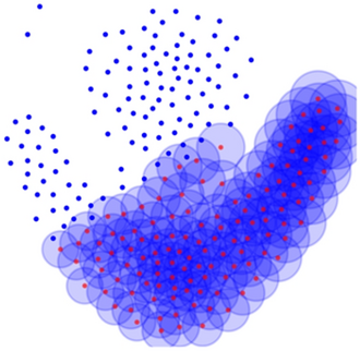

The process diagram of the blue class using Eq. (8) for diffusion and in order to reflect the diffusion process, the size of each point is reduced

Step 4: Overlapping the Ink Drops:

In this step, the degree of membership of the points belonging to this class can be obtained, which is calculated by aggregating the spread values of the data points of this class at this point. Considering that the degree of membership needs to be in the range of 0 to 1, so in order to ensure that all degrees of membership are within this range, the results obtained need to be processed. The simplest method is to calculate the average value of the membership function, as shown in Eq. (9). The overlapping effect of blue and red ink drops after diffusion are showed in Fig. 10.

Fig. 10

Diagram of the process of overlapping blue and red ink drops using Eq. (9)

${m}_{ij}({x}_{1},\dots {x}_{n})=\frac{1}{{N}_{i}}{\sum }_{j=1}^{{N}_{j}}{d}_{i}^{j}({x}_{1},\dots {x}_{n})$, and

$$\begin{array}{c}{m}_{ij}\left({x}_{1},\dots {x}_{n}\right)=1 if\, {m}_{ij}\left({x}_{1},\dots {x}_{n}\right)\ge 1\end{array}$$

(9)

where ${d}_{i}^{j}$ represents the ink drop function of the ith data point of class j, and ${N}_{j}$ represents the total number of data points of class j.

Step 5: Obtaining Fuzzy Membership:

This step is to put the membership degree of each data point obtained in step 4 into the position of the corresponding class in the matrix. The column i in the matrix represents the ith category, as shown in Eq. (10). After the above steps, the membership of the ith category can be filled into the ith column of the matrix.

$$\begin{array}{c}T= {\left[\begin{array}{cc}{m}_{11}& {m}_{12}\\ \vdots & \vdots \\ {m}_{N1}& {m}_{N2}\end{array}\right]}_{N\times 2}\end{array}$$

(10)

where N denotes the total number of data points.

Step 6: Iterating and Spreading Another Class:

In the next iteration, the same procedure is used to calculate the degree of membership belonging to another category, so as to obtain the data of another column in the matrix, thereby obtaining a complete membership matrix T.

Step 7: Defuzzification:

After diffusion, defuzzification is performed to obtain a new boundary between the normal class and the abnormal class. The defuzzification can be performed by taking the index i of the maximum value of each row of the membership function, as shown in Eq. (11). Figure 11 shows the classification of the Flame data set after defuzzification.

Fig. 11

The classification result after defuzzification using Eq. (11)

$$\begin{array}{c}{L}_{i}=\underset{\begin{array}{c}k=1,\dots ,K\\ i=1,\dots ,N\end{array}}{arg\mathrm{max}}\left({m}_{i,k}\right)\end{array}$$

(11)

The final classification results of some points may be different from the clustering results of the first step, which means that some points that belong to the normal traffic in the first step become abnormal at the end, and vice versa. This is because the ALM considers the influence of the shape and density of each point on the surrounding points, thereby improving the clustering results and therefore also improving the detection effect.

Since K-means has the characteristics of fast convergence speed, few parameters, and excellent performance in imbalanced classes, especially when dealing with data with high feature dimensions, it has the characteristics of strong model generalization ability and fast training speed. Although it is sensitive to outliers and noise points, it can be improved by combining the ALM algorithm. The K-means algorithm can better adapt to the high-dimensional feature vector of the network traffic, while ALM can perform fast calculations based on the matrix, so as to achieve accurate and efficient anomaly detection of the network traffic. Algorithm 1 describes the process of fuzzy modeling, and its main idea comes from IDS in ALM.

5 Experiment and Analysis

5.1 Experiment Dataset

In order to verify the anomaly detection method proposed in this paper, it is necessary to select appropriate network flow data. Although there are some public network security test datasets: DAPRA1998, UNSW_NB15, NSL-KDD, etc., there are many shortcomings and problems such as incomplete traffic, data anonymization, and outdated attack scenarios. Therefore, this article does not use these internationally known data sets to simulate the performance of the proposed algorithm.

The CICDDoS2019 dataset [44] is used in this paper to evaluate our proposed classifier, which makes up for the shortcomings and limitations of the previous datasets. It is a new data set generated by the Canadian Cyber Security Institute, which aims to design a real-time detector at low computational cost. The researchers analyze the new types of attacks that can be achieved at the application layer based on TCP/UDP protocol, and proposed a new classification of exploit attacks and reflection attacks, as shown in Fig. 10 below. The data set contains a total of 50,063,112 records, including 50,006,249 DDoS attacks and 56,863 normal samples. DDoS attacks include DNS, LDAP, MSSQL, NetBIOS, NTP, SNMP, SSDP, SYN, TFTP, UDP, UDP-LAG, and WebDDoS categories. More than 80 features were extracted from the data set using CICFLOWMeter tools. The details of the data set used in our experiments are shown in Table 1.

Table 1 CIDDDoS2019 dataset used in testing

5.2 Performance Indicators of Classification Model

For the detection classification model, it is necessary to use different evaluation index values to evaluate the performance of the model. This paper selects the confusion matrix of the classifier to evaluate the detection performance of the proposed model, as shown in Table 2.

Table 2 Confusion matrix

Specific evaluation indicators include:

• (1) True Positive: The number of normal network flows classified as normal by the model, represented by TP.

• (2) False Negative: The number of normal network flows classified as attack by the model, represented by FN.

• (3) False Positive: The number of attack network flows classified as normal by the model, represented in FP.

• (4) True Negative: The number of attack network flows classified as attack by the model, represented as TN.

Various indicators such as accuracy, precision, F1 score, recall, and False Positive Rate (FPR) are used to evaluate the proposed framework, which is defined in Eqs. (12)–(16).

$$\begin{array}{c}{\mathrm{Accuracy}}=\frac{\mathrm{TP}+\mathrm{TN}}{\mathrm{TP}+\mathrm{TN}+\mathrm{FP}+\mathrm{FN}}\end{array}$$

(12)

$$\begin{array}{c}{\mathrm{Precision}}=\frac{\mathrm{TP}}{\mathrm{TP}+\mathrm{FP}}\end{array}$$

(13)

$$\begin{array}{c}\mathrm{Recall}=\frac{\mathrm{TP}}{\mathrm{TP}+\mathrm{FN}}\end{array}$$

(14)

$$\begin{array}{c}{\text{F}}{1}-{\text{s}}{\text{c}}{\text{o}}{\text{r}}{\text{e}}=\frac{2\mathrm{TP}}{2\mathrm{TP}+\mathrm{FP}+\mathrm{FN}}\end{array}$$

(15)

$$\begin{array}{c}{\mathrm{FPR}}=\frac{\mathrm{FP}}{\mathrm{FP}+\mathrm{TN}}\end{array}$$

(16)

5.3 Experiment Result

In order to test the effectiveness of the proposed model, two experiments are designed. The first experiment detects each type of attack separately, and there are 11 types of attacks in total. The second experiment mixed multiple types of attack traffic to simulate the real traffic environment that may occur.

In the first experiment, considering that the proposed algorithm is based on the combination of K-means algorithm and ALM, the performance of this algorithm and K-means method is compared in the experiment. It is also compared with two other unsupervised learning methods, Auto-encoder and LSTM. In addition, we compare it with the supervised learning methods that have been shown in [45], such as: NB, SVM, and Decision Tree (DT).

The dataset of the second experiment is randomly generated, and there are a total of 4 data sets. Each data set is mixed with 11 kinds of attacks, and the proportion of each attack in the data set is randomly generated according to a normal distribution, as shown in Table 3. For example, in Dataset 1, DNS attack traffic accounts for 8.43% of all attack traffic, LDAP accounts for 8.46%, and so on. Similarly, a comparative experiment is also carried out, and the models used are: SVM, DT, and NB.

Table 3 Proportion of each attack data in the 4 mixed datasets

In the feature extraction module, the correlation between features can be represented by heat maps. The heat map in Fig. 12 shows the correlation between certain features of one of the data sets. The heat map uses the color of the corresponding location rectangle to represent the value. The darker the color, the greater the value. Among them, red indicates that the correlation between the features is + 1, and orange represents that it exceeds + 0.8, and both values reveal that there is a strong correlation between the features. Therefore, if the corresponding grid between a pair of features is red and orange, only one of them is kept.

Fig. 12

A heat map showing the correlation between features

Figure 13 shows the relative contribution ranking of features obtained by LightGBM. The figure shows the top 12 most important features and shows the importance of each feature. Among them, the characteristic value with the highest contribution rate is Source Port, reaching 35%; the second is Flow Bytes, with a contribution rate of 18%. And the contribution value of the twelfth feature Fwd PSH Flags is close to 0, so all subsequent features are removed. After the above processing, more than 40 feature sets will be processed into a feature set containing only 11 features.

Fig. 13

The importance of features derived from 10 rounds of LightGBM training

Figure 14 shows the process diagram of anomaly detection in the data set. Figure 14a is the result of using K-means to classify the data set, which is divided into 2 categories. Figure 14b is a picture after ALM fuzzies the K-means result (only one type of diffusion process is shown), and finally Fig. 14c is obtained after defuzzification. It can be seen that after processing, the distribution of blue and red points has changed.

Fig. 14

Anomaly detection process diagram on a data set

The comparison between the proposed model and three unsupervised methods: K-means, Auto-encoder and LSTM is shown in Figs. 15, 16, and 17. Figure 15 shows the performance of the model under a single type of attack, which is mainly evaluated by four indicators: (a) Accuracy, (b) F1 score, (c) Recall, and (d) FPR. The proposed model trained on the datasets gives an accuracy value in the range of 86.75–99.97%, while the accuracy values given by K-means, Auto-encoder and LSTM are in the range of 68.21–98.66%, 28.04–98.84%, 6.92–99.59%, respectively. On the F1 score indicator, the minimum value of ALM is 0.929, K-means is, Auto-encoder and LSTM are 0.811, 0.137, 0.068, respectively. Similar results are observed when the statistical tests are performed for Recall and FPR. This shows that the proposed algorithm is more stable than the three unsupervised methods of K-means, Auto-encoder and LSTM, and has a higher detection rate and lower false alarm rate in a statistical sense.

Fig. 15

Performance evaluation for the CIDDDoS2019 dataset. a Accuracy, b F1 score, c Recall, d FPR

Fig. 16

Comparison with the K-means on a Accuracy, b F1 Score, c Recall and d FRP on 4 datasets mixed with multiple attacks

Fig. 17

Comparison with the three unsupervised methods on a Accuracy, b F1 Score, c Recall and d FPRon 4 datasets mixed with multiple attacks

Figure 16 shows the performance comparison between the proposed model and K-means under a mixture of multiple attack types. It can be seen from the figure that K-means and the proposed model are relatively stable on the four datasets. The accuracy of K-means is above 89%, the F1 score is above 0.945, and the accuracy of the proposed model is above 90.2%, the F1 score is above 0.949; orange indicates that the algorithm has higher Accuracy, F1 score and Recall indicators than K-means, as shown in Fig. 16a, b, c. In addition, the false alarm rate of K-means is less than 0.64%, and the false alarm rate of the proposed model is less than 0.0128%; blue indicates that K-means is higher than the proposed algorithm in FPR index, as shown in Fig. 16d. The performance of the two is evenly matched, but the proposed model is better, especially in FPR, which has very important significance in practical applications.

The performances of the proposed method with another two unsupervised method under a mixture of multiple attack types are compared as presented in Fig. 17. Figure 17a shows the difference of Accuray. It can be seen that the performance of the proposed algorithm has been relatively stable, floating at 90%; while Auto-encoder and LSTM performed well on some data sets, and sometimes performed worse. The maximum value of the two algorithms on this index is 83.9%, which is smaller than the minimum value of the proposed algorithm. On the F1 score indicator, the proposed algorithm fluctuates around 0.99; while Auto-encoder fluctuates within the range of 0.255–0.867, the minimum value of LSTM is 0.572 and the maximum value does not exceed 0.91. Figure 17c shows the difference in Recall index for each method. The green part indicates that the performance of LSTM is better than that of Auto-encoder; similarly, the blue part indicates that the performance of the algorithm is better than that of LSTM. The results in Figs. 16 and 17 show that compared with the three unsupervised learning methods, the proposed model performs better on all four data sets.

The performance comparison between the proposed model and other literature models is shown in Figs. 18 and 19. Figure 18 shows the performance comparison between the proposed model and the SVM, DT and NB models in the case of a single type of attack. It can be seen that on the UDP and SYN datasets, the precision of the four models is almost the same, all of which are above 95%. However, the performance gaps between UDPLag, MSSQL, NetBIOS, and LDAP datasets are large, especially on UDPLag. On the UDPLag dataset, the precision of other models is 0, while the model proposed in this paper reaches 97.83%. On the MSSQL, NetBIOS and LDAP datasets, the precision of the proposed model is above 99.67%, and other comparison models are above 20.5%. Similar results can be observed for Recall and F1 score. The results suggest that the proposed model perform well on all 7 datasets, and it is a suitable model to consider in practical applications.

Fig. 18

Comparison with the three supervised methods on a Precision, b Recall and c F1 Score with six types attack

Fig. 19

Comparison with the three supervised methods on a Accuracy, b F1 Score, c Recall and d Recall on 4 datasets mixed with multiple attacks

Figure 19 shows the comparative results of the proposed model and the SVM, DT and NB models under a mixture of multiple attack types. In Accuracy and F1 score indicators, NB, DT and the proposed model are relatively stable; while in Recall and FPR, the NB model is unstable. The SVM model is unstable on all 4 indicators. The accuracy of the SVM model can reach up to 83.12% and the lowest can reach 28.46%. NB, DT and the proposed model are relatively stable in terms of accuracy. The accuracy of the DT model fluctuates around 77%, the accuracy of the NB model fluctuates around 82%, and the proposed model fluctuates around 90%. In terms of FPR indicators, other models have reached a maximum of 85.7%, while the model in this article is stable at about 0.01%. It can be seen from the comparison that the proposed model is more stable and has higher accuracy.

6 Conclusion

At present, in the detection of abnormal network traffic, there are problems such as high detection rate of supervised learning method but lack of labeled data, and the detection rate of unsupervised learning method changes with changes in detection application. In response to these problems, this paper proposes an anomaly detection model using K-means and ALM.

This method starts with analyzing the characteristics of the detection traffic, and uses a variety of methods such as variance and Pearson coefficient and LightGBM. to solve the problem of extracting the important traffic features in the detection network.

Subsequently, through the fuzzy theory of ALM, the classification results of the traditional method K-means are diffused. Therefore, more accurate detection results are obtained.

Finally, a simulation experiment of traffic anomaly detection was carried out on the newly released CICDDoS2019 data set, and compared with other methods under different indicators to testify the performance and effectiveness of the proposed method.

In this paper, starting from the characteristics of the data itself, the ALM fuzzification method is applied to the network traffic with high feature dimension and large amount of data. The classification model combined with ALM and K-Means takes into account the shape, distribution and density of the data itself, and can also enhance the elimination of noise and outliers, thereby improving the classification effect. It provides new ideas for the field of unsupervised methods.

References

Bhuyan, M.H., Bhattacharyya, D.K., Kalita, J.K.: Network anomaly detection: methods, systems and tools. IEEE Commun. Surv. Tutor. 16, 303–336 (2014)
H. Sagha and S.B. Shouraki, et al., Genetic ink drop spread, in 2008 2nd International Symposium on Intelligent Information Technology Application 2 (2008), 603–607.
Arunraj, N., Hable, R., et al.: Comparison of supervised, semi-supervised and unsupervised learning methods in network intrusion detection system (NIDS) application, Anwendungen und Konzepte der. Wirtschaftsinformatik 6, 10–19 (2017)
Al-Yaseen, W.L., Othman, Z.A., Nazri, M.Z.A.: Multi-level hybrid support vector machine and extreme learning machine based on modified K-means for intrusion detection system. Expert Syst. Appl. 67, 296–303 (2017)
Heller, K., Svore, K. et al.: One class support vector machines for detecting anomalous windows registry accesses.In: Proceedings of Workshop on Data Mining for Computer Security (2003)
Dromard, J., Owezarski, P.: Study and evaluation of unsupervised algorithms used in network anomaly detection. In: Proceedings of the Future Technologies Conference, vol. 1070, pp. 397-416 (2019)
Alauthaman, M., Aslam, N., et al.: A P2P Botnet detection scheme based on decision tree and adaptive multilayer neural networks. Neural. Comput. Appl. 29, 991–1004 (2018)
Saritas, M.M., Yasar, A.: Performance analysis of ANN and naive Bayes classification algorithm for data classification. Int. J. Intell. Syst. Appl. Eng. 7, 88–91 (2019)
Moustafa, N., Hu, J., Slay, J.: A holistic review of network Anomaly detection systems: a comprehensive survey. J. Netw. Comput. Appl. 128, 33–55 (2019)
Plonka, D.: FlowScan: a network traffic flow reporting and visualization tool, In: Proceedings of the USENIX 14th System Administration Conference LISA XIV, pp. 305–317 (2000)
Almomani, O.: A feature selection model for network intrusion detection system based on PSO GWO, FFA and GA algorithms. Symmetry 12, 1046 (2020)
Ambwani, T.: Multi class support vector machine implementation to intrusion detection. In: Proceedings of the International Joint Conference on Neural Networks vol. 3, pp. 2300–2305 (2003)
Yang, J., Deng, J., et al.: Improved traffic detection with support vector machine based on restricted Boltzmann machine. Soft. Comput. 21, 3101–3112 (2017)
Panda, M., Abraham, A., Patra, M.R.: Discriminative multinomial naive bayes for network intrusion detection, In: 2010 6th International Conference on Information Assurance and Security, pp. 5–10 (2010)
Taher, K.A., Jisan, B.M.Y., Rahman, M.M.: Network intrusion detection using supervised machine learning technique with feature selection. In: 2019 International Conference on Robotics, Electrical and Signal Processing Techniques, pp. 643–646 (2019)
Yin, C., Zhu, Y., et al.: A deep learning approach for intrusion detection using recurrent neural networks. IEEE Access 5, 21954–21961 (2017)
Wu, Z., Wang, J., et al.: A network intrusion detection method based on semantic re-encoding and deep learning. J. Netw. Comput. Appl. 164, 102688 (2020)
Arunraj, N., Hable, R., et al.: Comparison of supervised, semi-supervised and unsupervised learning methods in network intrusion detection system application, Anwendungen und Konzepte der. Wirtschaftsinformatik 6, 10–19 (2017)
Gamage, S., Samarabandu, J.: Deep learning methods in network intrusion detection: A survey and an objective comparison. J. Netw. Comput. Appl. 169, 102767 (2020)
Choi, H., Kim, M., et al.: Unsupervised learning approach for network intrusion detection system using autoencoders. J. Supercomput. 75, 5597–5621 (2019)
Vartouni, A.M., Kashi, S.S., Teshnehlab, M.: An anomaly detection method to detect web attacks using stacked auto-encoder, In: 2018 6th Iranian Joint Congress on Fuzzy and Intelligent Systems, (2018)
Vartouni, A.M., Teshnehlab, M., Kashi, S.S.: Leveraging deep neural networks for anomaly-based web application firewall. IET Inf. Secur. 13, 352–361 (2019)
Wu, D., Jiang, Z., et al.: LSTM learning with Bayesian and Gaussian processing for anomaly detection in industrial IoT. IEEE Trans. Industr. Inf. 16, 5244–5253 (2020)
Syarif, I., Bennett, A.P., Wills, G.: Unsupervised clustering approach for network anomaly detection, In: Networked Digital Technologies, Springer, Berlin, pp. 135–145 (2012)
MacQueen J.: Some methods for classification and analysis of multivariate observations. In: 15th Berkeley Symposium on Mathematical Statistics and Probability vol. 14, pp. 281–297 (1967)
Velmurugan, T., Santhanam, T.: Computational complexity between K-means and K-medoids clustering algorithms for normal and uniform distributions of data points. J. Comput. Sci. 6, 363 (2010)
Lu, W., Tong, H.: Detecting network anomalies using CUSUM and EM clustering. In: Proceedings of 4th International Symposium on Advances in Computation and Intelligence, Springer, pp. 297–308, (2009)
Knorr, E.M., Ng, R.T.: Finding intensional knowledge of distance-based outliers. Citeseer 99, 211–222 (1999)
Chimphlee, W., Abdullah, A. H.: Anomaly-based intrusion detection using fuzzy rough Clustering. In 2006 International Conference on Hybrid Information Technology, vol. 1, pp. 329–334 (2006)
Sharma, R., Chaurasia, S.: An enhanced approach to fuzzy C-means clustering for anomaly detection, In: Proceedings of 1st International Conference on Smart System, Innovations and Computing, pp. 623–636 (2018)
Hamamoto, A.H., Carvalho, L.F.: Network anomaly detection system using genetic algorithm and fuzzy logic. Expert Syst. Appl. 92, 390–402 (2018)
Zadeh, L.A.: Fuzzy logic. Computer 21, 83–93 (1988)
Murakami, M.: Practicality of modeling systems using the IDS method: Performance investigation and hardware implementation, PhD thesis in Electrical Engineering, Department of information Technology, the University of Electro-Communication (2008)
Firouzi, M., Shouraki, S.B., Afrakoti, I.E.P.: Pattern analysis by active learning method classifier. J. Intell. Fuzzy Syst. 26, 49–62 (2014)
Afrakoti, I., Shouraki, S.B., et al.: Using a memristor crossbar structure to implement a novel adaptive real-time fuzzy modeling algorithm. Fuzzy Sets Syst. 307, 115–128 (2017)
Shouraki, S.B., Honda, N.: Simulation of brain learning process through a novel fuzzy hardware approach, In: Proceedings of the IEEE International Conference on Systems, Man, and Cybernetics, vol. 3, pp. 16–21 (1999)
Merrikh-Bayat, F., Shouraki, S.B., Rohani, A.: Memristor crossbar-based hardware implementation of the IDS method. IEEE Trans. Fuzzy Syst. 19, 1083–1096 (2011)
Shouraki, S.B.: Recursive fuzzy modeling based on fuzzy interpolation, Journal of Advanced. Comput. Intell. 3, 114–125 (1999)
Afrakoti, I.E.P., Shouraki, S.B., Haghighat, B.: An optimal hardware implementation for active learning method based on memristor crossbar structures. IEEE Syst. J. 8, 1190–1199 (2014)
Murakami, M., Honda, N.: A study on the modeling ability of the IDS method: A soft computing technique using pattern-based information processing. Int. J. Approx. Reason. 45, 470–487 (2007)
Murakami, M.W., Honda, A.: basic constructive algorithm for the IDS method, In: Proceedings of the Joint 3rd International Conference on Soft Computing and Intelligent Systems and 7th International Symposium on Advanced Intelligent Systems, pp. 355–360 (2006)
Javadian, M., Shouraki, S.B., Kourabbaslou, S.S.: A novel density-based fuzzy clustering algorithm for low dimensional feature space. Fuzzy Sets Syst. 318, 34–55 (2017)
Javadian, M., Malekzadeh, A., et al.: A clustering fuzzification algorithm based on ALM. Fuzzy Sets Syst. 389, 93–113 (2020)
Sharafaldin, I., Lashkari, DA.H. et al.: Developing realistic distributed denial of service (DDoS) attack dataset and taxonomy, In: Proceedings of the 53rd International Carnahan Conference on Security Technology, pp. 1–8 (2019)
Vuong, T.H., Thi, C.V.N., Ha, Q.T.: N-Tier machine learning-based architecture for DDoS attack detection. Intell. Inform. Database Syst. 12672, 375–385 (2021)
Acknowledgements
The authors would like to thank the reviewers and editors for their valuable discussions and feedback. This work is supported in part by the open fund project of the Hunan Provincial Engineering Research Center of Electric Transportation and Smart Distribution Network (Changsha University of Science & Technology) (No. 3040102-1105008), and in part by the project of "Practical Innovation and Enhancement of Entrepreneurial Ability (No. 6080201-000101204)” for Professional Degree Postgraduates of Changsha University of Science &Technology.
Author information
Authors and Affiliations
Corresponding author
Rights and permissions
About this article
Cite this article
Liao, N., Li, X. Traffic Anomaly Detection Model Using K-Means and Active Learning Method. Int. J. Fuzzy Syst. 24, 2264–2282 (2022). https://doi.org/10.1007/s40815-022-01269-0
Received:
Revised:
Accepted:
Published:
Issue Date:
DOI: https://doi.org/10.1007/s40815-022-01269-0