
Abstract
This paper extends a schedule-based transit assignment model to integrate vehicle sharing systems (VSS) with or without fixed stations permitting one-way rentals. It is assumed that travelers receive information through mobile internet on vehicle location and availability and that they can use a real-time booking service. The proposed model extends the functionality of a scheduled-based transit assignment in two ways: (1) It generates intermodal route choice sets combining transit and non-transit trip legs. This functionality enables an accessibility analysis to identify od-pairs benefiting from VSS. (2) It distributes a given travel demand on the route choice set considering capacity constraints of VSS. This functionality can be applied for an impact analysis of a proposed VSS.
1 Motivation
Urban travel demand models typically cover the transport modes: car driver, car passenger, public transport, bike and walking. In the mode choice and route choice step they usually focus on unimodal trips and neglect intermodal trips. This is appropriate as today nearly all urban and regional trips employ just one mode of transport, if one does not consider the access and egress walk as an additional mode. In Germany the share of intermodal trips like park and ride, bike and ride and kiss and ride only accounts for 1.0–1.5 % of all trips. Following the vision of a connected mobility (Berger 2013) smartphones and mobile internet will facilitate various forms of shared mobility, which may substantially influence future mode choice, route choice and the share of intermodal trips. This also leads to new requirements for macroscopic travel demand models as sharing systems combine characteristics of public transport and private vehicles:
-
Traditional carsharing with a fixed pick up and return station: Station-based carsharing schemes (e.g. Stadtmobil in Germany, Zipcar in the US) work similar to traditional car rentals. They may reduce car ownership and thus influence mode choice. In a travel demand model traditional car sharing can be incorporated as a specific person group with limited car access.
-
Carsharing with or without fixed stations and one-way rentals: Free-floating carsharing schemes (e.g. car2go, DriveNow) without fixed station as well as station-based systems permitting one-way rentals provide more flexibility to the traveler. Travelers can use a car just for one single trip within a trip chain or they can combine public transport and car transport within one journey. Until now it is at least difficult to handle such intermodal trips in the mode and route choice step of a macroscopic travel demand model.
-
Bike sharing with or without fixed stations and one-way rentals: Bike sharing schemes (e.g. Vélib’ in Paris, Call-a-Bike in Germany) can provide alternative choices for short distance trips or for intermodal trips in combination with public transport. Like free-floating carsharing they are yet difficult to integrate in a travel demand model.
-
Carpooling or ride sharing: Here travelers share the same vehicle for one entire trip or a part of a trip. Smartphone-based communication services (e.g. flinc.org) may support spontaneous short term and short distance carpooling. This can increase the occupancy rate of private cars. Travel demand models with a particular mode for car passenger can integrate carpooling for the entire trip. Partial carpooling requires model extensions.
This paper focuses on a dynamic traffic assignment model integrating vehicle sharing systems (VSS) with or without fixed stations permitting one-way rentals. It is assumed that travelers receive information through mobile internet on vehicle location and availability and that they can use a real-time booking service (e.g. moovel.com). Traditional car sharing, park & ride with private vehicles or carpooling are not addressed in the paper. The influence of vehicle sharing systems on entire trip chains is also not considered. The proposed model extends the functionality of a scheduled-based transit assignment in two ways:
-
It generates intermodal route choice sets combining transit and non-transit trip legs. This functionality enables an accessibility analysis to identify od-pairs benefiting from VSS.
-
It distributes a given travel demand on the route choice set considering capacity constraints of VSS. This functionality can be applied for an impact analysis of a proposed VSS on route choice and sub-mode choice, i.e. the choice between vehicles of the public transport systems and the VSS.
As intermodal trips especially with VSS are rare, traditional household surveys with trip diaries fail to capture a reasonable large number of observations. In a 1 week trip diary in German cities with public bike sharing systems the 4500 surveyed persons reported almost 100,000 trips, but only 44 of these trips used the sharing system. And even in a control group of 450 registered users just 172 trips with the sharing system were reported. This low number of observations makes it difficult to calibrate a mode choice model or an assignment model with an integrated sub-mode choice. Therefore, the paper cannot provide results of a case study with a calibrated model based on real data. However, to estimate the parameters of such a model one would first need an assignment model capable to generate the set of alternative intermodal routes. The proposed method can provide this choice set.
Integrated in a travel demand model the proposed assignment model provides a tool for addressing various questions related to VSS:
-
Urban transport planners: What is the potential of VSS? Can VSS reduce the demand for on-street parking? Are dedicated parking lots for VSS necessary? How will they influence mode choice?
-
Public transport operators: Are VSS a threat to traditional public transport or can they extend the catchment area of public transport? Is it necessary to adapt the existing network?
-
VSS operators: How to design a VSS in terms of fleet size, operating area and fares? What revenues can be expected from a VSS?
The paper is organized as follows: After briefly describing the state of the art we present the underlying data model. Then we give an overview on the proposed model and explain the choice set generation. Using this choice set we present the route choice model distinguishing various approaches to consider capacity constraints of VSS.
2 State of the art
Vehicle sharing systems (VSS) can be integrated in macroscopic or in microscopic travel demand models. In a microscopic approach one would assume that the trips are modeled with their exact itinerary, i.e. with the arrival and departure times of each trip leg. In a macroscopic approach a VSS can be integrated in a frequency-based or in a schedule-based modeling approach. The number of publications on frequency-based and schedule-based transit assignment methods is large, but there are yet few publications on transit assignment including VSS.
Leurent (2013) suggests an extension of a frequency-based transit assignment. He treats the VSS mode as a specific kind of public service which provides station-to-station legs to the traveler. The model can handle one-way rentals with a station-based VSS. The access to a VSS vehicle considers the availability at the access station. The model likewise considers capacity constraints when returning a vehicle at a station. The assignment applies a method of successive averages to determine a state of equilibrium. At the time of publication the model development and testing were still in progress.
Ciari et al. (2013) present a model for estimating travel demand for carsharing using the activity-based microsimulation MATSim. They extend MATSim with an additional mode and apply a utility function which considers two of the fundamental features of a carsharing system: access to carsharing cars and the fare structure. The model assumes that “One agent can pick up the car only at one of the predefined stations, and must bring it back to the same one. Agents always choose the closest station to the starting facility. Agents walk to the pick-up point”. This limits the model application to traditional carsharing, which does not permit one-way rentals. The model which is applied for the Zurich region also assumes that an unlimited number of cars are available at the stations.
Romero et al. (2012) also study a multi-modal network design problem, but combine station-based VSS with the private car instead of transit. They start from the definition of a multi-modal network model for car and VSS, develop a combined mode and route choice model, and finally solve an optimization problem for locating the stations based on desired flows from the assignment.
Finally, numerous papers deal with the optimization of the day-to-day operation of VSS, notably with re-positioning strategies in one-way systems, which is outside the scope of this paper. A good overview of this literature is given in Vogel et al. (2014).
Most of these models deal only with the optimization of the supply side, take demand as exogenous input and model the demand reaction to changes in supply only very cursorily or not at all. One notable exception is (Rahul and Miller-Hooks 2014), who presents a bilevel model for a network design problem. The upper level maximizes the VSS operator’s revenue by varying station locations, fleet size, and initial vehicle deployment whereas the lower level captures the demand reaction by calculating an assignment of the (fixed) total demand to the combined VSS and public transport network. Rahul et al.’s approach differs from our work in several aspects:
-
We are interested primarily in studying network effects (such as changes in accessibility differentiated in time and space) of a VSS with (exogenously) given dimensions, whereas for Rahul the dimensioning of the VSS is the primary objective. Our model therefore only covers the lower level of Rahul, but at a higher level of detail and with more flexibility.
-
Our model can be applied to VSS with different operating regimes (station-based, free-floating, uncapacitated for sketch-level planning), whereas Rahul only treats the station-based case. The assignment method chosen for Rahul’s lower level [Optimal Strategies (Spiess and Florian 1989)] admits only link-additive costs, which limits the range of pricing schemes that can be studied. To overcome this limitation, the assignment method would have to be replaced by a different one, as suggested in the conclusion. In contrast, this work uses a route choice model in which the choice set contains complete od-paths from origin to destination, so that fares of any type can be represented at path level.
3 Data model
The multi-modal network of transport infrastructures and services is represented by means of a graph G = (N, A), where N is the set of nodes and A ⊆ N × N is the set of links, each representing a specific piece of infrastructure. Two subsets of links are distinguished: \(A = A^{T} \cup A^{\text{NT}}\) where \(A^{T}\) are called transit links (on which transit services run) and \(A^{\text{NT}}\) are called non-transit links (for access, egress, and transfers using other modes, including walking). A subset of nodes S ⊆ N, called stops, define locations where passengers can board and/or alight from transit services, e.g. a particular platform or curbside. Transfers within a single stop take zero time. If transfers require non-zero time, then the alighting and boarding stop are distinct nodes.
Demand is defined as the number of (traveler) trips between pairs of nodes. Trips start and end at nodes within a subset \(Z \subset N\), the set of zones. The complete study time period is partitioned into a set of non-overlapping time intervals T. The number of trips from origin zone u to destination zone v which depart during time interval t ∈ T is given by function \(d(u,v,t)\).
Transit services are organized in a set L of lines. A (directional) line ℓ∈L traverses an acyclic path k ℓ on the network, whose support links and nodes are denoted \(A_{\ell } \subseteq A^{T}\) and N ℓ. It serves in one direction an ordered set of stops, its stop sequence, denoted \(S_{\ell } \subseteq S \cap N_{\ell }\). Several lines can share the same nodes and links.
The generic line \(\ell \in L\) is characterized by:
-
a strictly positive running time \(t_{\ell }^{\text{run}} (s)\), for each line segment \(s \in S_{\ell } ,\)
-
a non-negative dwell time \(t_{\ell }^{\text{dwell}} (s)\), at each stop \(s \in S_{\ell }\).
Both running and dwell times are assumed to be deterministic. It would also be possible to make running and dwell times a function of volume. The same is true for capacity constraints in the transit network. Doing so would further increase the realism of the model, as the demand for VSS would be influenced by capacity bottlenecks in the transit network. As the capacity constraints in the VSS network already lead to an iterative solution method, this refinement would not increase the computational burden further. We omit the presentation for clarity, as the refinement does not change the structure of the solution method.
Each line \(\ell \in L\) is served by an ordered set of runs, its run sequence, denoted R ℓ. A run \(r \in R_{\ell }\) is constituted by one vehicle serving all stops of the line in order. We assume that each run \(r \in R_{\ell }\) has well-defined scheduled departure time \(\tau_{r}^{ + } (s)\) and arrival times \(\tau_{r}^{ - } (s)\) at all stops s ∈ S ℓ, at least in the form of a working timetable defined by the operator. Within our data model, only the scheduled departure time \(\tau_{r}^{ + } (s_{1} )\) from the first stop \(s_{1}\) is a specific property of a run, because it implicitly determines all other scheduled arrival and departure times downstream, through the line running and dwell times.
Transit vehicles have a finite capacity which affects passenger comfort and ability to board a given run. Here we choose to ignore congestion and capacity effects for transit services, because they do not affect the way in which transit and VSS are combined in the model, and because we want to avoid confusion with capacity effects in the VSS part of the model, which we do consider.
For access, egress, and transfers, travelers may use modes other than transit. In this paper we only consider exchangeable modes, i.e. walking or VSS. Private vehicles are not considered. The set of non-transit modes is denoted by M. For each link \(a \in A^{\text{NT}}\) and mode \(m \in M\) the link travel time \(t_{m} (a)\) is non-negative. If m is not permitted on a, \(t_{m} (a) = + \infty\). Some modes can be accessed only in specific locations, so-called stations. Beginning the use of mode m at node u (check-in) takes non-negative time \(t_{m}^{ + } (u)\), ending the use (check-out) takes time \(t_{m}^{ - } (u)\), e.g. for unlocking or dropping off a shared vehicle. If mode m is not accessible at node u (e.g. a station-based VSS without a station at node u), then \(t_{m}^{ + } (u) = t_{m}^{ - } (u) = + \infty\). Applying these definitions to a free-floating VSS mode m, essentially all walk-accessible nodes would allow access to VSS mode m. Because this would lead to a combinatorial explosion in connection search, we adopt an alternative model for such modes. Only the nodes in \(S \cup Z\) (stops and zones) allow access. They are called virtual stations of mode m and represent a discretization of the true situation. Later sections explain how connection search and utility calculation compensate for the discretization.
To keep track of available capacity, particularly for free-floating VSS, the total service area is partitioned into a set G of non-overlapping regions. A region is not a traffic analysis zone, but an additional object which similar to a zone is defined by a polygon and which records the number of available vehicles. Each station u is assigned to exactly one region \(g \in G\). The surface area of region g is denoted by a (g). The number of available vehicles of mode m in region g at the beginning of time interval t is denoted as \({\text{veh}}_{m} (g,t)\). While \({\text{veh}}_{m} (g,t)\) is endogenous for later time intervals, the initial distribution \({\text{veh}}_{m} (g,t_{0} )\) is input to the model.
For a journey from an origin to a destination node travelers choose a connection with a discrete departure and arrival time using a particular spatial route. This connection consists of several legs each describing a part of the journey with just one means of transport, i.e. a specific vehicle or walking. A leg is always described by a spatial route. As long as a leg only contains information on the route we call it route leg. After assigning a departure and an arrival time to a route leg we then call it connection leg. The term path refers to a specific sequence of nodes in graph G. If the path represents an entire connection we call it od-path. This leads to the following formal definitions:
A connection from node u to node v is an ordered sequence of connection legs: \({\text{cx}}(u,v) = ({\text{cl}}_{1} (w_{11,} w_{12} ), \ldots ,{\text{cl}}_{k} (w_{k1,} w_{k2} ))\) where \(u = w_{11} ,w_{k2} = v,w_{j2} = w_{j + 1,1} ,{\text{for}}\,j = 1..k - 1\). Each leg has a departure time \(\tau^{ + } ({\text{cl}})\) and an arrival time \(\tau^{ - } ({\text{cl}})\). For successive legs \({\text{cl}}_{i} ,{\text{cl}}_{i + 1}\) of a connection, \(\tau^{ - } ({\text{cl}}_{i} ) \le \tau^{ + } ({\text{cl}}_{i + 1} )\) holds. A connection leg is either a transit leg or a non-transit leg. A transit leg is a triple \({\text{cl}}(u,v) = (r,u,v)\) and covers a transfer free ride using a specific run \(r \in R_{\ell }\) from stop u to stop v, with \(\tau^{ + } ({\text{cl}}) = \tau_{r}^{ + } (u),\tau^{ - } ({\text{cl}}) = \tau_{r}^{ - } (v)\). A non-transit leg from node u to node v is a pair \({\text{cl}}(u,v) = (m,p)\) where \(m \in M\), p is a non-transit path from u to v on \(A^{\text{NT}}\), and \(t_{m}^{ + } (u),t_{m}^{ - } (v),t_{m} (a)\;\forall a \in p\) are all finite. The arrival time of a non-transit connection leg is derived from the departure time, the link travel times along the od-path and the times for check-in and check-out: \(\tau^{ - } ({\text{cl}}) = \tau^{ + } ({\text{cl}}) + \sum\nolimits_{a \in p} {t_{m} (a)} + t_{m}^{ + } (u) + t_{m}^{ - } (v).\)
The fare of connection leg cl is given by non-negative function \(\varPhi ({\text{cl}})\) and the fare for connection cx is given by \(\varPhi ({\text{cx}}) = \sum\nolimits_{cl \in cx} {\varPhi ({\text{cl}})}\). This is a simplification which ignores fare schemes in which tickets may cover multiple legs.
The set of connection legs CL provides the input for generating the choice set of connections. Each connection leg cl is derived from a route leg rl which only describes the spatial course of a connection leg. Different from a connection leg a route leg does not contain a departure and arrival time. Transit and non-transit connections legs are computed in different ways:
-
Transit connection legs can be computed in a preprocessing step. Figure 1 (top) explains the construction of all transit route legs belonging to one line ℓ. Combining each run of line ℓ with the route legs of this line creates the set of connection legs of this line.
Fig. 1 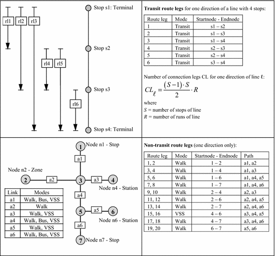
Construction of route legs (transit and non-transit) and transit connection legs of a line
-
Non-transit connection legs can only be determined during the construction of the connection choice set as their departure and arrival time depends on the public transport timetable. The preprocessing step only determines route legs. The set of non-transit route legs for mode walking contains all time-shortest paths between the zone nodes and the stop nodes, the zone nodes and the VSS station nodes and between the stop nodes and the VSS station nodes. The size of the set can be limited by defining a maximum walking time. The set of non-transit route legs for each VSS mode contains all time-shortest paths between the VSS station nodes. Figure 1 (bottom) illustrates the construction of non-transit route legs.

4 Assignment model
4.1 Model overview
The following sections describe a dynamic, multi-modal assignment model in which the VSS part can consist of any number of station-based or free-floating VSS. Combinations of both principles within one VSS are possible, i.e. within a core area a VSS may operate free-floating, whereas throughout the rest of the service area access is limited to stations. Travelers obtain information about vehicle availability and routing to the nearest available vehicle or free dock for check-out by querying a real-time booking service. They also reserve the nearest available vehicle. This set of assumed characteristics implies that walk access time to/from the VSS vehicle and availability of a vehicle for check-in and a dock for check-out are stochastic variables only at query time. Once the passenger chooses a route, it can be executed deterministically, i.e. without risk of failure or delay in the VSS part.
Access times and vehicle availability depend not only on the capacity of the VSS, but also on the demand for it, which leads to a capacity-constrained assignment model. The proposed solution method involves fixed-point iteration. The first subsection below explains choice set generation (connection search), assuming that access times are known. Then we describe the generalized cost calculation and the route choice model, which uses balancing factors in order to satisfy capacity constraints. It also defines how access times and balancing factors are updated for the next iteration based on assigned traveler volumes.
4.2 Choice set generation
For generating the set CX of all potential connections we extend the time-dependent, multi-path algorithm described by (Friedrich and Wekeck 2004). This algorithm builds a connection tree, which may contain several od-paths (connections) from the origin to every destination node. Figure 2 outlines the structure of the connection tree. The root of the tree is the centroid node of the origin zone and the only outgoing branch represents a walk access from the origin to the nearest public transport stop. If there are more stops or VSS stations in the vicinity of the origin node additional walk legs are added. Once all legs of one level are inserted the depth of the tree is increased to the next level. Here again all suitable legs are inserted according to the rules described below. The width of the final connection tree depends mainly on the service frequency of the lines. The use of entire connection legs as tree edges simplifies the tree’s structure to a great extent and limits its depth to a low number which primarily depends on the number of transfers.

Structure of the connection tree
Constructing the connection tree requires the definition of a search impedance \(I({\text{cx}})\) for a connection cx:
where \(t^{\text{tt}}\) is the travel time of the connection, \(n^{\text{trans}}\) the number of transfers between public transport vehicle, \(n^{\text{VSS}}\) the number of legs using VSS and \(\varPhi\) the fare. \(\alpha^{\text{tt}}\), \(\alpha^{\text{trans}}\), \(\alpha^{\text{VSS}}\) and \(\alpha^{\text{cost}}\) are global user-defined parameters. This search impedance function is similar to the utility function used in the subsequent route choice step. While the utility reflects the perception of the travelers, the impedance is used to generate an appropriate choice set. This can justify a somewhat different function and different parameter values.
Starting from the origin node \(u_{0}\), a branch & bound strategy is employed. At each node the connection tree is branched by adding legs connecting the current node to successor nodes. Node specific values for the maximum travel time \(t^{\text{tt}}\) and the maximum number of transfers \(n^{\text{trans}}\) serve as an upper bound. The arrival time determines a lower bound for the earliest departure time of a subsequent leg. In this way only potentially suitable legs are inserted thus limiting the width of the tree. Given a connection leg from the current tree level, all possible successors are considered. Let \({\text{cl}}^{*} (u,v)\) be the currently processed connection leg starting at network node \(u\) and terminating at network node \(v\). Let \({\text{cx}}^{*} (u_{0} ,v)\) be the new connection between the \(u_{0}\) and \(v\) formed by adding \({\text{cl}}^{*} (u,v)\) to connection \({\text{cx}}^{*} (u_{0} ,u)\) arriving at \(u\). Finally, let \({\text{CX}}(u_{0} ,v)\) be the set of all known connections from the origin node to v.
\({\text{cl}}^{*} (u,v)\) is inserted into the tree as an extension of connection \({\text{cx}}^{*} (u_{0} ,u)\), if the following conditions hold:
-
Temporal suitability: The connection leg \({\text{cl}}^{*} (u,v)\) departs from node \(u\) only after the arrival of connection \({\text{cx}}^{*} (u_{0} ,u)\):
-
$$\tau^{ - } ({\text{cx}}^{*} (u_{0} ,u)) \le \tau^{ + } ({\text{cl}}^{*} (u,v))$$(2)
.
-
Sequential test (optional): A VSS connection leg may only be inserted before the first or after the last transit leg.
-
Dominance: There is no known connection \({\text{cx}} \in {\text{CX}}(u_{0} ,v)\) such that
-
\(\tau^{ - } ({\text{cx}}) \ge \tau^{ - } ({\text{cx}}^{*} (u_{0} ,v))\) and \(\tau^{ + } ({\text{cx}}) \le \tau^{ + } ({\text{cx}}^{*} (u_{0} ,v))\) and \(I({\text{cx}}) \le I({\text{cx}}^{*} (u_{0} ,v))\)
-
and \(n^{\text{trans}} ({\text{cx}}) \le n^{\text{trans}} ({\text{cx}}^{*} (u_{0} ,v))\) and \(n^{\text{VSS}} ({\text{cx}}) \le n^{\text{VSS}} ({\text{cx}}^{*} (u_{0} ,v))\).
In other words, if \({\text{cx}}^{*} (u_{0} ,v)\) has the property that for all known connections \({\text{cx}}\) from origin to \(v\), \({\text{cx}}^{*} (u_{0} ,v)\) departs later or arrives earlier or has a lower impedance or a lower number of transfers or uses VSS less frequently than \({\text{cx}}\), \({\text{cx}}^{*} (u_{0} ,v)\) will be inserted.
-
Tolerance constraints: None of the following rules is violated:
$$I({\text{cx}}^{*} (u_{0} ,v)) \le b_{1} \cdot \min_{{{\text{cx}} \in {\text{CX}}(v)}} I({\text{cx}}) + b_{2}$$(3)$$t^{\text{tt}} ({\text{cx}}^{*} (u_{0} ,v)) \le d_{1} \cdot \min_{{{\text{cx}} \in {\text{CX}}(v)}} t^{\text{tt}} ({\text{cx}}) + d_{2}$$(4)$$n^{\text{trans}} ({\text{cx}}^{*} (u_{0} ,v)) \le e_{1} \cdot \min_{{{\text{cx}} \in {\text{CX}}(v)}} n^{\text{trans}} ({\text{cx}}) + e_{2}$$(5)$$n^{\text{trans}} ({\text{cx}}^{*} (u_{0} ,v)) \le {\text{MAXNT}}$$(6)where all \(b_{i}\), \(d_{i}\) and \(e_{i}\) are user-specified global tolerance parameters and \({\text{MAXNT}}\) is the also user-defined bound for the number of transfers within a connection.Loops: Transfers within one transit line are only allowed for lines containing a loop, provided that the passenger can save time by boarding an earlier service trip at the intersection node of the route loop.
A tree level is traversed completely before connection legs of the next level are considered. The procedure terminates when the queues are empty or the maximum number of transfers is reached.
All generated connections are grouped by departure time: \({\text{CX}}(u,v,t) = \left\{ {{\text{cx}} \in {\text{CX}}(u,v)|\tau^{ + } ({\text{cx}}) \in t} \right\}\). Finally, for each time interval t one additional connection with an arbitrary departure time is inserted into CX (u, v, t) which contains only non-transit legs using the shortest non-transit path.
4.3 Utility calculation and route choice
The overall form of the proposed route choice model is standard: For each \(u,v \in Z,t \in T\) a multinomial logit model splits demand d (u, v, t) across the alternatives in the choice set CX (u, v, t), constructed above, based on a utility function defined on CX (u, v, t). Details of the model formulation for transit, including aspects like the similarity between alternatives or optional Box-Cox transformations of travel time components, can be found in (Friedrich and Wekeck 2004) and (Leurent 2013). Although there is reason to expect that Cross-Nested Logit better reflects correlations between alternatives, recent work (van der Gun et al. 2014) indicates that these formulations lead to estimation problems. Here we give a summary and then focus on the treatment of VSS within the model.
The utility of a connection cx with k legs \({\text{cl}}_{1} , \ldots ,{\text{cl}}_{k}\) is given by
where
\(n^{\text{trans}}\) equals the number of transit legs minus one, and \(U({\text{cl}}_{k} )\) is the utility of leg k. Likewise \(n^{\text{VSS}}\) equals the number of connection legs including a VSS.
If \({\text{cl}} = (r,u,v)\) is a transit leg of cx, then
The general formulation for the utility of a non-transit leg \({\text{cl}} = (m,p)\) is given by
where \(\omega_{m}^{{}} (u,t)\) is a non-negative balancing factor which penalizes excess demand for check-outs (available vehicles) at station u during interval t. For station-based VSS the same approach can be used to penalize excess demand for check-ins (available docks). We omit this here for brevity, because it does not alter the structure of the model.
Consider the special case where a walk leg precedes a leg of a free-floating VSS. It connects a zone or a stop to a virtual station. Since these two legs are by construction co-located at the same node u, the access walk time cannot be determined from link attributes. Instead the virtual station represents any potential location of an available VSS vehicle in the vicinity of the zone/stop, and the time for walk access must be calculated as a function of vehicle density. Note that the expected (average) walk time is not a good basis for the utility. If the traveler plans a trip which contains a VSS leg prior to a transit leg, then she will include a safety margin in order to reach the transit stop in time for the transfer. This is better expressed by a higher than average percentile of walk access time, where the exact percentage depends on the risk-averseness of the traveler. For the calculation of the percentile assume that stop/zone u is assigned to region g, and \({\text{veh}}_{m} (g,t)\) is the number of available vehicles in g at t. Consider a small subregion \(g^{\prime} \subset g\) surrounding u. If vehicle locations are distributed independently and uniformly over g, then
Solving (11) for \(a(g^{\prime})\), given \(a(g)\), \(n = {\text{veh}}_{m} (g,t)\), and a probability p, yields.
This is the surface area of a region in which the traveler will find an available vehicle with probability p. If \(g^{\prime}\) is circular, then the maximum walk time for reaching any point in \(g^{\prime}\) is
where \(v_{\text{walk}}\) is the walk speed and \(\gamma\) is a detour factor. For the purpose of connection search and utility calculation we fix a probability \(p^{*}\) as an average safety margin.
The primary results of the assignment are traveler volumes q (cx) for each connection. By tracing each cx through the network, secondary results are derived, including \(q_{m}^{ + } (u,t)\) = number of check-ins at station u in interval t, \(q_{m}^{ - } (u,t)\) = number of check-outs at u in t, and \(\tilde{t}_{m} (t)\) = average duration of a leg of mode m in t.
The model formulation admits different forms of access to VSS and different levels of detail at which capacity constraints can be taken into account.
4.3.1 VSS with unlimited capacity
In the simplest case capacity constraints are ignored completely for mode m. This assumption may be useful in a study of VSS potential, where the objective is to identify the total latent demand for a VSS under optimal conditions and its spatial and temporal distribution. In this case we set \(\omega_{m}^{{}} (u,t) = 0,\forall u,t\).
We do not treat the free-floating case, because with unlimited capacity walk access time to the nearest available vehicle would either be undefined or zero, in which case VSS degenerates to a form of walking.
Assignment in this case terminates after a single iteration, because none of the variables are flow-dependent.
From the assignment result it is possible to derive the required fleet size under optimal conditions as
where \(\left\| t \right\|\) = duration of time interval t.
4.3.2 VSS with system capacity
In this case we assume that the VSS service area consists of a single region g with fleet size \({\text{veh}}_{m} (g,t)\) for mode m, constant over all t. The number of vehicles constrains the total number of check-outs per time interval. We postulate, however, that these check-outs can occur anywhere in the network and that VSS vehicles are perfectly re-positioned between uses. This assumption can be used to derive a theoretical upper bound on the demand, which can be served with a given fleet, as a baseline for assessing the efficiency of re-positioning strategies. The capacity constraint in this case will not affect route choice within the VSS part, but will drive excess demand for VSS to VSS-free alternative routes. In this case all balancing factors for a given time interval t are set to the same constant which is re-evaluated in each iteration: \(\omega_{m}^{{}} (u,t) = \omega_{m} (t),\forall u,t\). Note that route choice within VSS does not change, because the MNL model is sensitive to utility differences, and the utility of each VSS leg is decreased by the same amount.
Furthermore if m is free-floating, we set \(t_{\text{walk}} = t_{\text{walk}} ({\text{veh}}_{m} (g,t),g,p^{*} )\) for each walk leg cl preceding a mode m leg. This corresponds to the assumption that due to finite system capacity walk access will be necessary to reach the nearest available vehicle of m, but due to re-positioning the walk time will only depend on system vehicle density, not on the spatio-temporal distribution of demand.
To satisfy the capacity constraints, balancing factors are updated after each iteration of the assignment. The maximum possible number of check-outs during time interval t equals \({\text{cap}}_{m} (t) = {\text{veh}}_{m} \cdot \frac{\left\| t \right\|}{{\tilde{t}_{m} (t)}}\). If \(\sum\nolimits_{u} {q_{m}^{ + } (u,t) > {\text{cap}}_{m} (t)}\) for a time interval t, Newton’s method is used to find \(\omega_{m}^{*} > 0\) such that \(q_{m}^{ + } (u,t) - {\text{cap}}_{m} (t) = 0\). This value is then used as \(\omega_{m} (t)\) for the next iteration, i.e. the utility of any VSS-using path is decreased to the point where the capacity is exactly exhausted. The iterations of Newton’s method require multiple evaluations of the choice model, but fortunately the computational effort for this is much lower than for the choice set generation which is not repeated.
4.3.3 Station-based VSS with station capacity
In this variant we keep track of available vehicles for each station and time interval. The initial distribution of vehicles \({\text{veh}}_{m} (u,t_{0} )\) is given as input. The assignment model is evaluated in chronological order. From the results for time interval t, update
for all stations u.
We consider the capacity constraint for station u to be satisfied, if for each time interval t: \({\text{veh}}_{m} (u,t) \ge 0\). Note that the condition is only enforced at discrete timepoints, and it is optimistically assumed that check-ins and check-outs in between these balance in a feasible manner. Similar to the case with system capacity, if the constraint is violated for given \(u,t_{i}\), then Newton’s method is used to find values \(\omega_{m}^{*} (u,t_{i} ) > 0\) for which \({\text{veh}}_{m} (u,t) = 0\), perfectly exhausting capacity. This calculation is performed simultaneously for all stations, as diverting passengers from one oversaturated station may drive another station over capacity.
4.3.4 Free-floating VSS with region capacity
In this variant, available vehicles are only tracked at the level of regions. Otherwise the treatment is completely analogous to the station-based case. Given the initial distribution of vehicles to regions, \({\text{veh}}_{m} (g_{j} ,t_{0} )\), vehicle availability is updated according to
Where capacity constraints are violated within a region \(g_{j}\), balancing factors \(\omega_{m}^{{}} (g_{j} ,t_{i} )\) are computed for the region, then assigned identically to each virtual station inside \(g_{j}\).
Access walk time to a virtual station within region \(g_{j}\) is set to \(t_{\text{walk}} ({\text{veh}}_{m} (g_{j} ,t),g_{j} ,p^{*} )\).
4.4 Iteration control
The convergence check at the end of each iteration consists of two conditions:
(17) states that demand for check-outs nowhere exceeds capacity, and (18) states that connection volumes are stable. Unless (17) and (18) are satisfied or a user-defined maximum number of iterations has been reached, the next iteration is executed with updated balancing factors and walk times to virtual stations.
5 Example
Consider the small example in Fig. 3 which illustrates some effects of the model. Zones 1 and 2 are connected by a network with a train and a bus line, and travelers have a choice of two VSS routes as an alternative to the bus leg. Travel times are given in Table 1 (symmetrical). Transfer wait time is 5 min between train and bus. Fares are 5.0 for the train, 0.8 for the bus, 4.0 for VSS. The assignment period runs from 7:00 to 10:00, subdivided into three time intervals of 1 h length each, denoted 7–8, 8–9, 9–10. Demand per time interval from Zone 1 to Zone 2 is 100, 25, 100, respectively, and from Zone 2 to Zone 1 it is 25, 100, 100.

Example network with traveler volumes in a unconstrained and b capacity-constrained case
The utility function is given by
The coefficients are arbitrarily chosen, as no survey data were available to estimate the model. Results therefore illustrate the mechanics of the model and do not reflect actual observations. Figure 3a shows the traveler volumes in each time interval resulting from an unconstrained assignment. A proportion of travelers choose VSS, because it is faster than the bus connection, although the fare is higher. Of those travelers that choose VSS, about two-thirds use the route via V1, because it is shorter than via V3. As demand from Zone 1 to Zone 2 is equal in the first and third time interval the link volumes in this direction are also equal in these time intervals in the unconstrained case.
For a second model run assume that the number of VSS vehicles is limited to 16, of which initially 4 are located at V1, 4 at V2, 8 at V3. The model with station capacities first solves the assignment for interval 7–8, starting without capacity constraint. Assigned volume in this starting solution (identical to Fig. 3a) exceeds capacity at V1, so balancing factors \(\omega\) are iteratively computed to decrease volumes until they just match capacities. At convergence the volumes shown in Fig. 3b for the time interval 7–8 are obtained. It can be seen that the number of check-ins at V1 is reduced from 9.3 to 4.0, which exhausts the capacity. Some of the demand diverts to the VSS route via V3 where check-ins increase slightly from 6.3 to 6.6. The capacity constraint at V3 is not violated, because remaining travelers take the bus. Nevertheless because of the capacity constraint the longer VSS route captures more demand than the shorter route. Based on check-ins/outs during the time interval 7–8, capacities are updated for the assignment of the next time interval 8–9. Example: for V2 the capacity in 8–9 is 4.0 − 3.9 + 10.6 = 10.7. With these capacities the constrained assignment is calculated for time interval 8–9. In this time interval demand from zone 2 to zone 1 is high. VSS usage is limited to 10.7 (essentially those vehicles brought there by travelers from zone 1 during 7–8). Unlike previously at stop B, vehicles near zone 2 are now concentrated at a single VSS station (V2), so the route split in the reverse direction follows the route travel times, the majority of demand being captured by the route via V1. Finally the process is repeated for time interval 9–10, where demand is high in both directions. VSS usage is capacity-constrained at all three VSS stations, but most severely at V2 where only few vehicles arrived during time interval 8–9.
The balancing factors for each station and time interval can be converted back into additional fares and interpreted as congestion shadow prices. In the example these additional fares are 0.90 for V1 in 7–8, 0.43 for V2 in 8–9, and even 1.51 for V2 in 9–10.
6 Conclusion
VSS are trendy. Many people expect VSS to improve urban mobility and contribute to a more sustainable urban transport. Others are more skeptical. They believe that the impact of VSS is overrated or that it may threaten public transport. At the moment the share of trips using VSS is small and has no measureable impact on other modes. In Stuttgart, a German city with 600,000 inhabitants, 500 electric car2go Smart cars, a traditional car sharing scheme with 400 vehicles and 400 public bikes every day approximately 3000–4000 trips are performed with shared vehicles. This number is high enough to notice the vehicles in traffic and while parking. Nevertheless the trips only contribute a share of 0.1–0.2 % of all trips. And more than 80 % of the trips are unimodal, i.e. they are not combined with public transport. As most VSS are privately operated it is often difficult to get comprehensive data on the usage of VSS. Schmöller and Bogenberger (2014) report differences in the usage of free-floating car sharing in Munich compared to reports by Kortum (2012) describing the usage in Austin, Texas. The differences refer to the peak hours and the trip purposes with more rentals for leisure trips in the evening and on weekends in Munich. Nevertheless one can expect a change in use pattern of free-floating carsharing as the systems are still rather new. The changing use pattern and the low number of VSS trips, however, explain why it is difficult to observe VSS trips through a traditional household survey with trip diaries, even if the sample just contains registered VSS users. Without observations it remains difficult to estimate the parameters of a utility function for VSS mode choice or sub-mode choice within an assignment. As a start one may use parameter values observed for public transport, especially in places where surveys indicate that VSS replace public transport trips. Alternatively one could conduct stated choice experiments. As VSS are usually more expensive than public transport it is important to precisely address the impact of the fares.
Despite the low share of VSS and the problems of modeling modes with low shares planners and decision makers will request tools for analyzing and forecasting the impacts of VSS. The presented approach can support this in various ways:
-
It can generate a choice set with transit and non-transit legs. The choice set generation method can also be applied to microscopic models.
-
It can identify od-pairs benefiting from VSS.
-
It can estimate the number of users depending on the number of stations or vehicles.
-
It can approximate the numbers of daily users per vehicle.
-
It can indicate the demand for redistribution resulting from uneven temporal and spatial demand pattern.
-
It can provide insight on the impacts of large-scale VSS.
The model described above was tested for small examples using the PTV Visum software complemented by a Python script. It may serve as a specification for an implementation in a future release. Based on the experience of the schedule-based transit assignment with capacity constraints, which is already implemented in Visum, we expect that the model will be applicable for large-scale applications in urban areas. Different from a dynamic and stochastic highway assignment model only the loading step needs to be repeated in each iteration. As the set of connections does not depend on the network loading one connection search step is sufficient.
References
Berger R (2013) Connected Mobility 2025. http://www.rolandberger.de/media/pdf/Roland_Berger_TaS_Connected_Mobility_E_20130123.pdf. Accessed 18 July 2014
Ciari F, Schuessler N, Axhausen KW (2013). Estimation of carsharing demand using an activity-based microsimulation approach: model discussion and some results. In: International Journal of Sustainable Transportation, No 7, Taylor & Francis, 2013, pp 70–84
Friedrich M, Wekeck S (2004). A schedule-based transit assignment model addressing the passengers’ choice among competing connections. In: Schedule-based dynamic transit modeling: theory and applications. Kluwer Academic Publishers, 2004, pp 159–173
Kortum, K (2012). Free-floating Carsharing Systems: Innovations in Membership Prediction, Mode Share, and Vehicle Allocation Optimization Methodologies, Dissertation, University of Texas at Austin, 2012
Leurent, F (2013). Travel Demand for a One-Way Vehicle Sharing System: a model of traffic assignment to a multimodal network with supply-demand equilibrium. In: Proceedings of the 3rd International Conference on Models and Technologies for Intelligent Transportation Systems 2013. Dresden, 2013
Rahul N, Miller-Hooks E (2014). Equilibrium network design of shared-vehicle systems. In: European Journal of Operational Research 235, pp 47–61
Romero JP, Ibeas A, Moura JL, Benavente J, Alonso B (2012) A Simulation-optimization Approach to Design Efficient Systems of Bike-sharing. In: Proceedings of 15th Meeting of the EURO Working Group on Transportation, September 2012, Paris, Elsevier
Schmöller S, Bogenberger K (2014) Analyzing external factors on the spatial and temporal demand of car sharing systems. Procedia-Soc Behav Sci 111(2014):8–17
Spiess H, Florian M (1989) Optimal strategies: a new assignment model for transit networks. Transp Res Part B 23B(2):83–102
Van der Gun JP, Van Nes R, Van Arem B (2014) Flexible public transport modelling for large urban areas. In: hEART 2014: 3rd Symposium of the European Association for Research in Transportation, Leeds, UK
Vogel P, Ehmke JF, Mattfeld DC (2014). Decision support for tactical resource allocation in bike sharing systems. TU Braunschweig Institute report 2014. https://www.tu-braunschweig.de/Medien-DB/winfo/publications/decision_support_for_tactical_resource_allocation_in_bike_sharing_systems.pdf. Accessed 25 Jul 2014
Author information
Authors and Affiliations
Corresponding author
Rights and permissions
About this article

Cite this article
Friedrich, M., Noekel, K. Modeling intermodal networks with public transport and vehicle sharing systems. EURO J Transp Logist 6, 271–288 (2017). https://doi.org/10.1007/s13676-015-0091-7
Received:
Accepted:
Published:
Issue Date:
DOI: https://doi.org/10.1007/s13676-015-0091-7