
Abstract
Multiple orthogonal polynomials with respect to two weights on the step-line are considered. A connection between different dual spectral matrices, one banded (recursion matrix) and one Hessenberg, respectively, and the Gauss–Borel factorization of the moment matrix is given. It is shown a hidden freedom exhibited by the spectral system related to the multiple orthogonal polynomials. Pearson equations are discussed, a Laguerre–Freud matrix is considered, and differential equations for type I and II multiple orthogonal polynomials, as well as for the corresponding linear forms are given. The Jacobi–Piñeiro multiple orthogonal polynomials of type I and type II are used as an illustrating case and the corresponding differential relations are presented. A permuting Christoffel transformation is discussed, finding the connection between the different families of multiple orthogonal polynomials. The Jacobi–Piñeiro case provides a convenient illustration of these symmetries, giving linear relations between different polynomials with shifted and permuted parameters. We also present the general theory for the perturbation of each weight by a different polynomial or rational function aka called Christoffel and Geronimus transformations. The connections formulas between the type II multiple orthogonal polynomials, the type I linear forms, as well as the vector Stieltjes–Markov vector functions is also presented. We illustrate these findings by analyzing the special case of modification by an even polynomial.
1 Introduction
Multiple orthogonality is a very close topic to that of simultaneous rational approximation (simultaneous Padé aproximants) of systems of Cauchy transforms of measures. The history of simultaneous rational approximation starts in 1873 with the well known article [28] in where Charles Hermite proved the transcendence of Euler’s constant e. Later on, along the years 1934-35, Kurt Mahler delivered in the University of Groningen several lectures [35] where he settled down the foundations of this theory. In the mean time, two Mahler’s students, Coates and Jager, made important contributions in this respect (see [19, 30]).
There are two formulations of multiple orthogonality, the so called type I and type II ones, see [42]. Both are equivalent in the sense of the duality. If we set a problem involving orthogonality conditions regarding several measures (or several weights) we call it a type II problem. Under this view, the fundamental objects are polynomials. The dual objects for these polynomials are linear forms considered in the type I version of multiple orthogonality. Due to the fact that perhaps type II version is more natural, the research interest has been centered in the characterization of this type of systems (cf. [5]).
The Angelescu and the Nikishin [4, 38, 43] are the two main systems of multiple orthogonal polynomials that have been discussed in the literature. Contributions regarding zero distribution, interlacing property and confinement of the zeros, are studied in [21, 25, 27, 31,32,33,34]. Multiple orthogonal polynomials also have different expressions for the Christoffel–Darboux kernel, coming from the different ways of defining them from the recurrence relation [20, 22, 41]. Studying the asymptotic behavior of this kernel is essential in the study of universality classes in random matrix theory due to its connection with eigenvalue distribution. Recent trends of multiple orthogonal polynomials can be seen in [29]. For multiple Gaussian quadratures see [15, 22] and for Laguerre–Freud equations, Darboux transformations and related perturbations see [11,12,13,14, 37]. Laguerre–Freud equations play a key role in the study of the coefficients of the three term recurrence relation satisfied by monic standard orthogonal polynomials [14] and see also [37] for the so called structure relation.
Multiple orthogonal polynomials can be built recursively, once we choose a chain of indexes. In [1] the chain of indexes is given through the generalized Euclidean division, and using the Gauss–Borel factorization of the related matrix of moments we find that the type I and type II orthogonality conditions appear now clearly related through bi-orthogonality conditions.
In [6, 44] multiple orthogonal polynomials with respect to p weights satisfying Pearson’s differential equation are studied, giving a classification of type II multiple orthogonal polynomials that can be represented by a product of commuting Rodrigues type operators.
This paper is devoted to the study of multiple orthogonal polynomials with two weights on the step-line, also known in the literature as 2-orthogonal polynomials in the case of type II (see [36], among others). In the research on the relation between Markov chains beyond birth and death processes and multiple orthogonal polynomials [17, 18] we get, as a byproduct, some results that hold for families of these type I and II simple cases. Moreover, in order to better understand some of these phenomena we turned back to the definition of multiple orthogonality and find, to the best of our knowledge, some unknown facts so far. Given their general character and interest, we decided to collect them in a separate publication. Let us now give an account of the contents of this paper.
First we apply the Gauss–Borel factorization described in [1]. Within this description we introduce, associated to the lower and upper triangular factors of the moment matrix, two matrices J and \({\tilde{J}}\) having the sequences of orthogonal polynomials of type II and type I, respectively, as eigenvectors. The first one is the recursion matrix, which happens to be a banded matrix with four non-vanishing diagonals, the first superdiagonal, the main diagonal and the two first subdiagonals. However, \({\tilde{J}}^\top \) is not a band matrix but an upper Hessenberg matrix so that all its superdiagonals, but for the first one, are zero. Nevertheless, its square \({\tilde{J}}^2\) happens to be equal to the transpose of J and, consequently, is a banded matrix. These relations lead to expressions of the matrix \({\tilde{J}}\) in terms of the four nonzero diagonals of the recursion matrix J. This is described in Sect. 1.2.
In Sect. 1.3 it is shown that for multiple orthogonal polynomials the recursion matrix J, or equivalently the sequence of type II multiple orthogonal polynomials \(\{B^{(n)}\}_{n=0}^\infty \), related to the spectral system \((w_1,w_2,{\text {d}}\mu )\), determines uniquely \(w_1\). However, the second weight \(w_2\) is not uniquely determined. We describe this phenomena as a gauge freedom. It is also shown that the type I linear form associated to the sequence of type II multiple orthogonal polynomials \(\{B^{(n)}\}_{n=0}^\infty \) is also uniquely determined. Examples of this gauge freedom with almost uniform Jacobi matrices are obtained in [18].
In Sect. 2 we assume that the two weights \((w_1,w_2)\) satisfy first order scalar Pearson equations, as it does for instance the Jacobi–Piñeiro. We are able to find in the matrix setting a symmetry for the matrix of moments and derived a Laguerre–Freud matrix, a finite band matrix with only four nonzero diagonals, that accounts for the consequences. These ideas lead to differential equations satisfied by the multiple orthogonal polynomials of type II as well as for the corresponding linear forms of type I.
Then, in Sect. 3 we deal with a nice symmetry easily described in this two-component case. There is a relation between the moment matrices with weights \((w_1,w_2)\) and \((xw_2,w_1)\), that we call permuting Christoffel symmetry. The connection matrix for both multiple orthogonal polynomials of type II and linear forms of type I is remarkably simple in this case. We will apply it to the case of Jacobi–Piñeiro multiple orthogonal polynomials [39, 42], that we take as case study. This provides explicit formulas connecting the polynomials and linear forms with parameters \((\alpha ,\beta ,\gamma )\) and \((\beta ,\alpha +1,\gamma )\). We also present the Christoffel formula when the transformation is the multiplication of both weights by x, with no permutation. Both types of Christoffel transformations are relevant in the understanding of the mentioned uniform Jacobi matrices related to hypergeometric weights see [1]. Then, motivated by the previous examples we analyze the general Christoffel and Geronimus transformations for a system of weights \((w_1,w_2)\), and we end the paper by taking the modification by an even polynomial as a case study of these two type of transformations.
1.1 Two component multiple orthogonal polynomials on the step-line
We present here well basic results regarding multiple orthogonal polynomials, see for example [42]. We follow the Gauss–Borel factorization problem approach of [1]. We consider

and, in terms of a system of a couple of weights \(\mathbf {w} = (w_1,w_2)\), the vector of monomials

we define the following vector of undressed linear forms

Definition 1
For a given measure \(\mu \) with support on \(\Delta \), an interval in \({\mathbb {R}}\), and weights \(w_1\) and \(w_2\) as above, the moment matrix is given by
Definition 2
The Gauss–Borel factorization of the moment matrix g is the problem of finding the solution of
with S, \({\tilde{S}}\) lower unitriangular semi-infinite matrices

and H a semi-infinite diagonal matrix with diagonal entries \(H_l\ne 0\), \(l\in {\mathbb {N}}_0\).
Let us assume that the Gauss–Borel factorization exists, that is, the system \((\mathbf {w},{\text {d}}\mu )\) is perfect. In terms of S and \({\tilde{S}}\) we construct the type II multiple orthogonal polynomials
with \(m \in {\mathbb {N}}_0\), as well as the type I multiple orthogonal polynomials
and
For \(m \in {\mathbb {N}}_0\), the linear forms are
Proposition 1
(Type I and II multiorthogonality relations) In terms of the weight vectors, \(\mathbf {\nu } (2 m) =(m+1,m)\) and \(\mathbf {\nu }(2m+1)=(m+1,m+1)\), \(m \in {\mathbb {N}}_0\), and corresponding multiple orthogonal polynomials
the following type I orthogonality relations
for \(j\in \{0,\ldots , |\mathbf {\nu }|-2\}\), and type II orthogonality relations
are fulfilled.
Defining

the lower unitriangular factors S, \({\tilde{S}}\) can be written in terms of its subdiagonals as follows
with \(S^{[k]},{\tilde{S}}^{[k]}\) diagonal matrices with entries \(S^{[k]}_l, {\tilde{S}}^{[k]}_l\), \(l\in {\mathbb {N}}_0\), respectively. Hence,
so that \(\displaystyle B^{(m)}=x^m+\sum _{i=0}^{m-1}S^{[m-i]}_{i} x^i \) and
Definition 3
Vector of type II multiple orthogonal polynomials and of type I linear forms associated with \((w_1, w_2,{\text {d}}\mu )\) are defined, respectively, by


Proposition 2
(Biorthogonality) The following multiple biorthogonality relations
hold.
1.2 Recurrence relations and the shift matrices
Definition 4
(Shifted matrices) We introduce the following shift matrices

with

From this definition we get the following technical lemma that determines the algebra of the multiple orthogonality studied in this work.
Lemma 1
The shift matrices satisfy
as well as
Moreover, the projection matrices

satisfy
Proposition 3
(Bi-Hankel structure of the moment matrix) The moment matrix fulfills the symmetry condition
Remark 1
Therefore, it satisfies a bi-Hankel condition
and we can write the moment matrix in terms of
as the following vectorial Hankel type matrix

Proposition 4
(Recursion matrix) The matrix
is a Hessenberg matrix of the form

and T is a tetradiagonal matrix.
Theorem 1
(Recursion relations)
-
(i)
The recursion matrix, type II multiple orthogonal polynomials, and corresponding type I multiple orthogonal polynomials and linear forms of type I fulfill the eigenvalue property
$$\begin{aligned} { T } \, B&= x \, B,&{ T } ^\top A_1&= x \, A_1,&{ T } ^\top A_2&= x \, A_2,&{ T } ^\top Q&= x \, Q. \end{aligned}$$(15)Componentwise, this eigenvalue property leads to the recursion relations.
-
(ii)
The lower Hessenberg matrix
$$\begin{aligned} \hat{ { T } }&:=H^{-1} \tilde{ { T } } H,&\text {with }&\tilde{ T }&:={\tilde{S}} \Lambda {\tilde{S}}^{-1}, \end{aligned}$$is such that
$$\begin{aligned} { T } ^\top = \hat{ { T } }^2, \end{aligned}$$(16)and has the following eigenvalue property
$$\begin{aligned} {\hat{T}} \, A_1&= x \, A_2,&{\hat{T}} \, A_2&= A_1. \end{aligned}$$(17)Moreover, if \( { T }_1 : = H^{-1} {\tilde{S}} \Lambda _1 {\tilde{S}}^{-1} H\) and \( { T } _2 : =H^{-1}{\tilde{S}} \Lambda _2 {\tilde{S}}^{-1} H\), then
$$\begin{aligned} { T } _1 \, A _1= x \, A_1,&{ T } _2 \, A _2&= x \, A_2 , \end{aligned}$$(18)as well as,
$$\begin{aligned} { T } _1 \, A _2= \mathbf{0} ,&{ T } _2 \, A _1=\mathbf{0} . \end{aligned}$$
Proof
Equation (16) follows from the representation of T in Proposition 4 and taking into account (11). From
we deduce (17).
To deduce (18) use (12) and the definition of \(A_1\) and \(A_2\) in (9). \(\square \)
Remark 2
-
(i)
Despite \( {\hat{T}} \) is not a banded matrix, its square \(\hat{ { T } }^2\) is a tetradiagonal matrix.
-
(ii)
Consequently, we obtain the spectral equations
$$\begin{aligned} \hat{ { T } }^2 A_1&= x \, A_1,&\hat{ { T } }^2 A_2&= x \, A_2. \end{aligned}$$ -
(iii)
Notice that \(\hat{ { T } }^2= { T } ^\top = { T } _1 + { T } _2 \). Moreover \( { T } _1{ T } _2 = { T } _2{ T } _1 = \mathbf{0} \) so that for any polynomial p(x) we have \(p( { T } ^\top )=p( { T } _1 + { T } _2 )=p( { T } _1 )+p( { T } _2 )\).
Definition 5
(Shift operators) The shift operators \({\mathfrak {a}}_\pm \) acts over the diagonal matrices as follows
Lemma 2
Shift operators have the following properties,
for any diagonal matrix D.
A simple computation leads to:
Proposition 5
The inverse matrix \(S^{-1}\) of a lower unitriangular matrix S expands in terms of subdiagonals as follows
with first few subdiagonals \(S^{[-k]}\) given by
Lemma 3
For the recursion matrix
we have
Proof
We consider
Now, from Proposition 5 we get the desired representation. \(\square \)
Lemma 4
We have the following diagonal expansion
Proof
Observe that
so that
Hence,
and, as \(\hat{ { T } }^2=H \tilde{ { T } }^2 H^{-1}\), we get the announced result. \(\square \)
Theorem 2
For the recursion matrix given in (14) written in terms of its diagonals \( { T } = \Lambda + I b+\Lambda ^\top c+(\Lambda ^\top )^2d\), with b, c, d diagonal matrices from (16), we get
as well as
Proof
Use the previous two lemmas. \(\square \)
Corollary 1
We have
Proof
It follows form \(({{\mathfrak {a}}}_-^2H)d=H\). \(\square \)
Finally, to end this section, we discuss on the Christoffel–Darboux (CD) kernels, see [40] for the standard orthogonality, and corresponding CD formulas in this multiple context. The two partial and complete CD kernels are given by
These kernels satisfy Christoffel–Darboux formulas. Sorokin and Van Iseghem [41] derived a CD formula that can be applied to multiple orthogonal polynomials, see also [20, 22]. In Theorem 1 of [9] a CD formula for the mixed case was proven. Daems–Kuijlaars’ CD formula, that is not in sequence, was derived in [23, 24]. The extension to partials kernels follow the ideas of [9]. The CD formula reads as follows
as well as the partial CD formulas, for \(a\in \{1,2\}\), are
1.3 Hidden symmetry
In this section we explore further the connection of the system of weights \((w_1,w_2,{\text {d}}\mu )\) and the recursion matrix and its sequences of multiple orthogonal polynomials of type II and linear forms of type I.
In particular we discuss on a hidden symmetry already remarked in [22]. For multiple orthogonal polynomials the recursion matrix T, the sequence of type II multiple orthogonal polynomials \(\{B^{(n)}\}_{n=0}^\infty \), and even the sequence of type I linear forms \(\{Q^{(n)}\}_{n=0}^\infty \) do not determine uniquely the spectral system \((w_1,w_2,{\text {d}}\mu )\), as it determines uniquely \(w_1\), for the second weight one has the hidden freedom described below.
Proposition 6
Let \(\Delta \subset {\mathbb {R}}\) be the compact support of two perfect systems, \((w_1, w_2,{\text {d}}\mu )\), with \(\int _\Delta w_1(x) {\text {d}}\mu (x) =1\) and \(({{\hat{w}}}_1,{{\hat{w}}}_2,{\text {d}}\mu )\), with \(\int _\Delta {\hat{w}}_1(x) {\text {d}}\mu (x) =1\), that have the same sequence of type II multiple orthogonal polynomials \(\{B^{(n)}(x)\}_{n=0}^\infty \). Then \( {{\hat{w}}}_1 = w_1\) and there exists \(\alpha ,\beta , \gamma \in {\mathbb {R}}\), \(\alpha ,\beta \not =0\) such that
If \(A^{(m)}_1\), \(A^{(m)}_2\) are the type I multiple orthogonal polynomials, associated with the system \((w_1, w_2,{\text {d}}\mu )\), then the type I multiple orthogonal polynomials, \({\hat{A}}^{(m)}_1,{\hat{A}}^{(m)}_2\) associated with the system \((w_1,{{\hat{w}}}_2,{\text {d}}\mu )\) are given by
and both systems have the same linear associated forms
Proof
For \(B=S X\), the Gauss–Borel factorization (3) leads to
In terms of the projection matrices \( \Pi _1 \) and \(\Pi _2\), we split (26) as follows
Assuming \(\int _\Delta w_1(x) {\text {d}}\mu (x) =1\) and recalling that Sg is an upper triangular matrix we get

and we conclude that given S, the moments \(\int _\Delta x^n w_1 {\text {d}}\mu (x) \) are uniquely determined, and as the Hausdorff moment problem when solvable is determined, we obtain that \( {{\hat{w}}}_1 = w_1\).
Similarly, we get

We can assure that b and \({{\hat{b}}}\) are different from zero, otherwise \((w_1,w_2 , {\text {d}}\mu )\) and \((w_1,{{\hat{w}}}_2 , {\text {d}}\mu )\) would not be perfect systems. Then, we can find \(\alpha ,\beta , \gamma \), where \(\alpha , \beta \not =0 \) such that

Therefore,

which implies

and as the Hausdorff moment problem is determined we get (25).
Now, we consider the sequence of type I linear form associated to the system \((w_1, w_2,{\text {d}}\mu )\)
then it holds, that
Using the biorthogonality of the linear form, that the degree of the polynomial \( A_2^{(m)}\) is less than or equal to the degree of the polynomial \( A_1^{(m)}\), and the uniqueness of the type I polynomials associated to the perfect system \((w_1, {\hat{w}}_2,{\text {d}}\mu )\) we recover that \( {\hat{A}}^{(m)}_1=A^{(m)}_1- \frac{\gamma }{\alpha } A_2^{(m)} \) and \({\hat{A}}^{(m)}_2= -\frac{\beta }{\alpha } A_2^{(m)} \), and also that both systems have the same sequence of type I linear form associated \( {\hat{Q}}^{(m)} = Q^{(m)} \) as we wanted to prove. \(\square \)
2 Pearson equation and differential equations
Notice that the Jacobi–Piñeiro weights, \({\tilde{w}}_a (x)=w_a(x)(1-x)^\gamma \), \(a\in \{1,2\}\), i.e.
fulfill the following Pearson equations
as well as
Let us assume that \({\text {d}}\mu =v(x){\text {d}}x\), denote \({\tilde{w}}_a=w_a v\) with \(v(x) = (1-x)^\gamma \), and consider the following Pearson relations
where for the Jacobi–Piñeiro case we have \(\sigma (x)=x(1-x)\), \(q_1(x)=(\alpha (1 - x) -\gamma x)\), \(q_2(x)=(\beta (1 - x) -\gamma x)\), with \(\sigma \) a polynomial such that \(\sigma {\tilde{w}}_1=\sigma {\tilde{w}}_2=0\) at the boundary \(\partial \Delta \) of the support. If we introduce the notation
the Pearson equations are
On the other hand, to handle derivatives of type II multiple orthogonal polynomials we introduce the matrices

Proposition 7
The derivative of the vector of monomials is
The following identity
is satisfied.
Proof
This relation can be checked directly, from the explicit for of the matrices or by observing that

and the result follows. \(\square \)
On the other hand, to deal with derivatives of type I multiple orthogonal polynomials, we require of the matrices

Lemma 5
We have
Definition 6
Let us introduce
Lemma 6
The following relations are fulfilled
We also have
Theorem 3
If the Pearson equations (28) hold, then the following symmetry for the moment matrix
is fulfilled.
Proof
Observing
we deduce that
Integrating by parts we get
Hence, recalling that \(\sigma (x){\tilde{w}}_1(x)=0\) and \(\sigma (x){\tilde{w}}_2(x)=0\) at the boundaries of the support, we obtain
Then, the Pearson equations (27) lead to
and we conclude that
Finally, recalling that
and that
we obtain (30). \(\square \)
Definition 7
Let us define
Remark 3
-
(i)
The matrices \(\Phi ,\Phi _1\) and \(\Phi _2\) model the derivatives of the multiple orthogonal polynomials as follows
$$\begin{aligned} B'&=\Phi B,&A_1'&=\Phi _1 A_1,&A_2'&=\Phi _2 A_2. \end{aligned}$$Moreover, we have
$$\begin{aligned} \Phi _1 A_2&= \mathbf{0},&\Phi _2 A_1&= \mathbf{0}. \end{aligned}$$ -
(ii)
They also satisfy
$$\begin{aligned} \Phi _1 { T } _2 = { T } _2 \Phi _1=\Phi _2 { T } _1 = { T } _1\Phi _2= \mathbf{0}. \end{aligned}$$ -
(iii)
The matrices \(\Phi \), \(\Phi _1\) and \(\Phi _2\) are strictly lower triangular. The first possibly non zero subdiagonal of \(\Phi \) is the first one and of \(\Phi _1\) and \(\Phi _2\) the second one.
-
(iv)
We also have
$$\begin{aligned}{}[ { T } , \Phi ]&= { I } . \end{aligned}$$ -
(v)
Introducing the lower triangular matrices \(C_1=H^{-1} {\tilde{S}} \, \Pi _1 {\tilde{S}}^{-1} H\) and \(C_2=H^{-1} {\tilde{S}} \, \Pi _2 {\tilde{S}}^{-1} H\), that are projections \(C_1^2=C_1\), \(C_2^2=C_2\), \(C_1C_2=C_2C_1\) and \(C_1+C_2= { I } \), we have
$$\begin{aligned}{}[ { T } _1 , \Phi _1]&=C_1,&[ { T } _1 , \Phi _2]&=C_2,&[ { T } _1 + { T } _2 ,\Phi _1+\Phi _2]= { I} . \end{aligned}$$
Now, using the Gauss–Borel factorization, we are ready to express the symmetry for the moment matrix (30) in the following terms
Theorem 4
We have
Proof
Using the Gauss–Borel factorization \(g=S^{-1} H {\tilde{S}}^{-\top }\) of the moment matrix g we can write (30) as follows
so that
from where we get (31). \(\square \)
Definition 8
We introduce the Laguerre–Freud matrix
Proposition 8
The Laguerre–Freud matrix \(\Psi \) is a banded matrix with \(\deg \sigma -1\) possible non zero superdiagonals and \(2\max (\deg \sigma -1,\deg q_1,\deg q_2)\) possibly non zero subdiagonals.
Proof
This follows from (31). Indeed, the highest non zero superdiagonal of \(\Psi =\sigma ( { T } )\Phi \) is the \((\deg \sigma -1)\)-th one, and the lowest subdiagonal of \(\Psi =-\big ( \Phi _1 \sigma ( { T } _1 ) + \Phi _2 \sigma ( {T} _2 ) +q_1( {T} _1 ) +q_2( {T} _2 ) \big )^\top \) is \(2\max (\deg \sigma -1,\deg q_1,\deg q_2)\)-th one. \(\square \)
Theorem 5
In terms of the Laguerre–Freud matrix we have:
-
(i)
The type I multiple orthogonal polynomials fulfill
$$\begin{aligned} \sigma (x) A_1'(x)+q_1(x) A_1(x)+\Psi ^\top A_1(x)&= \mathbf{0}, \nonumber \\ \sigma (x) A_2'(x)+q_2(x) A_2(x)+\Psi ^\top A_2(x)&= \mathbf{0}. \end{aligned}$$(32) -
(ii)
The linear form \({\tilde{Q}}(x)=A_1(x){\tilde{w}}_1(x)+A_2(x){\tilde{w}}_2(x)=Q(x) v(x)\) is subject to
$$\begin{aligned} \sigma {\tilde{Q}}'(x)+\Psi ^\top {\tilde{Q}}(x)= \mathbf{0}. \end{aligned}$$(33) -
(iii)
The type II orthogonal polynomials satisfy
$$\begin{aligned} (\sigma (x)B(x))'=\Psi B(x). \end{aligned}$$(34)
Proof
From (31) we deduce that \(A_1\) fulfills
For \(A_2\) we proceed analogously. For the linear form we have
where we have used the Pearson equations (28). Then, from (32) the relation (33) for the linear form \( {\tilde{Q}}\) follows. Moreover, for the multiple orthogonal polynomials of type II we get that B is subject to
which completes the proof. \(\square \)
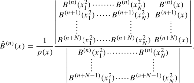
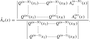
In terms of the determinants

we have:
Proposition 9
For a support \(\Delta =[a,b]\), a quadratic polynomial \(\sigma (x)=-(x-a)(x-b)\), \(\deg q_1=\deg q_2=1\), the Laguerre–Freud matrix has the following nonzero coefficients
Proof
From \(\Psi =\sigma ( { T } )\Phi \) we have that the first superdiagonal of \(\Psi \) is
and from \(\Psi =-\big ( \Phi _1\sigma ( { T } _1 ) + \Phi _2\sigma ( { T } _2 ) +q_1( { T } _1 ) +q_2( { T } _2 ) \big )^\top \) using (29) we get that the second subdiagonal is the transpose of
From (34) we deduce that
so that, as a, b are zeros of \(\sigma \)
Thus, as \(\sigma '(a)=-\sigma '(b)=(b-a)\), we get
These two equations can be written, for \(n\ge 2\) as

Therefore, we get

and the result is proven. \(\square \)
Remark 4
Therefore, the Laguerre–Freud matrix has the following structure

Remark 5
Componentwise Eq. (33) for the linear forms \(\{{\tilde{Q}}^{(k)}(x)\}_{k=0}^\infty \) is
Equation (34) for the type II orthogonal polynomials \(\{B^{(k)}(x)\}_{k=0}^\infty \) reads componentwise as follows
Remark 6
The Jacobi–Piñeiro case corresponds to the particular choice \(a=0\) and \(b=1\) and \(\sigma =x(1-x)\). Moreover, according to [17]
and, consequently,the determinants involved are
Remark 7
In [5, Corollary 2] the authors prove that the type II, multiple orthogonal polynomials that admits a Rodrigues formula representation, satisfies a \(p+1\) order differential equations of type
with explicitly given polynomial coefficients \(\displaystyle q_{k,p+1}\) that could depend on \(\displaystyle n\). In the case of Jacobi–Piñeiro, and for a system of two weight functions \(\displaystyle {\tilde{w}}_1, {\tilde{w}}_2\) we have, as \(p = 2\), a third order differential equation with polynomial coefficients given by,
In the proof the author’s heavily used the Rodrigues type formula representation for these polynomials.
We think that this technique cannot be used to derive the third order differential equations for the vector of type I linear forms. Nevertheless, by duality of the one derived in [5] for the type II multiple orthogonal polynomials of Jacobi–Piñeiro, we think that this can be achieved.
3 Christoffel and Geronimus perturbations: Christoffel formulas
We will start by considering basic simple cases and then we move to more general polynomial perturbations.
Definition 9
(Permuting Christoffel transformation) Let us consider \(\mathbf {w}=(w_1,w_2)\) and the transformed vector of weights \( \mathbf {{\underline{w}}} =(w_2, x \, w_1)\), that is a simple Christoffel transformation of \(w_1\) followed by a permutation of the two weights.
Proposition 10
(Permuting Christoffel transformation and the moment matrix) The moment matrix satisfies
Proof
In fact, we successively have
which completes the proof. \(\square \)
Remark 8
Observe that iterating (35) we get
and bi-Hankel property (13) of the moment matrix is recovered. In this sense the transformation \(\mathbf {w} \rightarrow \mathbf {{\underline{w}}} \) can be understood as a square root of the Christoffel transformation \(\mathbf {w}\rightarrow x\mathbf {w}\).
Let us assume that \(g_{ \mathbf {{\underline{w}}} }\) has a Gauss–Borel factorization
Definition 10
We introduce the connection matrix
Then,
Theorem 6
(Permuting Christoffel transformation) The connection matrix can be written as follows

The following connection formulas hold true
Proof
The Gauss–Borel factorization of (35) leads to
so that
Thus, we deduce that the matrix \(\Omega \) is an unitriangular matrix with only its first subdiagonal different from zero as well as the corresponding subdiagonal coefficients.
Moreover, from definition we get
Now,
Finally,
which ends the proof. \(\square \)
We now discuss similar connection formulas but for the CD kernels.
Proposition 11
For \(n\in {\mathbb {N}}\), the CD kernels (22) satisfy
Proof
Given any semi-infinite vector C or matrix M we will denote by \(C_{[n]}\) or matrix \(M_{[n]}\) the truncations, where we keep only the first n rows or n rows and columns (the indices will run from 0 up to \(n-1\)), respectively. Then, given the band form of \(\Omega \) we find

with \(C^{(n)}\) the corresponding entry of the vector C.
For \(a\in \{1,2\}\), we can write (22) using he following vector notation:
Then, using (37), (38) and (39) we deduce
so that using (41) and back again (42) we obtain the desired result. \(\square \)
Lemma 7
For \(n\in {\mathbb {N}}_0\), we have \(A_1^{(n)}(0)\ne 0\).
Proof
If \(A_1^{(n)}(0)= 0\), from (40) we deduce that \(K_{{\mathbf {w}},1}^{(n)}(x,0)=0\). Attending to (22) we have \(K_1^{(n)}(x,0)=\sum \limits _{m=0}^{n-1}B^{(m)}(x)A_1^{(m)}(0)\), as the sequence \(\{B^{(n)}(x)\}_{n=0}^\infty \) is linearly independent we deduce that \(A_1^{(m)}(0)=0\), for all \(m\in \{0,1,\dots ,n\}\), therefore \(A_1^{(0)}(0)=0\), which is impossible. \(\square \)
Lemma 8
For \(n\in {\mathbb {N}}_0\), the matrix coefficient \(\Omega _{n+1,n}\) of \(\Omega \) is
Proof
In the first relation in Eq. (38) put \(x=0\) and clean up to get the form of the unknown \(\Omega _{n+1,n}\). \(\square \)
Theorem 7
(Christoffel formulas) For \(n\in {\mathbb {N}}_0\), the type I orthogonal polynomials and linear forms fulfill
For \(n\in {\mathbb {N}}_0\), the type II orthogonal polynomials satisfy
For \(n\in {\mathbb {N}}_0\), we find
Proof
We just evaluate (40) and (24) at \(x=0\), use (43) and do some clearing. \(\square \)
Definition 11
The Jacobi–Piñeiro multiple orthogonal polynomials, correspond to the choice \(w_1=x^\alpha \), \(w_2:=x^\beta \) and \({\text {d}}\mu =(1-x)^\gamma \) with \(\alpha ,\beta ,\gamma >-1\) and \(\alpha -\beta \not \in {\mathbb {Z}}\), \(\delta =[0,1]\).
Theorem 8
(Permuting Christoffel transformation for Jacobi–Piñeiro I) The transformation \((\alpha ,\beta )\rightarrow (\beta ,\alpha +1)\) in the Jacobi–Piñeiro case has as connection matrix

The corresponding connection formulas
hold.
In [17] the explicit expressions for the Jacobi–Piñeiro’s \(H_n\) were given as
Then,
Corollary 2
(Permuting Christoffel transformation for Jacobi–Piñeiro II) The connection coefficients are explicitly given by
In terms of which we have the following connection formulas between Jacobi–Piñeiro multiple orthogonal polynomials with permuted parameters
We go back to Remark 8 and consider the basic Christoffel transformation
The following Lemma was first presented in [22, 7, Lemma 2.4], see also [16, Theorem 9]
Lemma 9
(Coussement-Van Assche) For \(n\in {\mathbb {N}}_0\), there are nonzero constants \(C_n\) such that

Proof
Despite this was proven elsewhere [22], for the reader convenience, we give a proof of it. In the one hand, we have that
 . On the other hand for
\(k\in \big \{0,\dots ,\lfloor \frac{n-1}{2}\rfloor \big \}\) we have
. On the other hand for
\(k\in \big \{0,\dots ,\lfloor \frac{n-1}{2}\rfloor \big \}\) we have

and for \(k\in \big \{0,\dots ,\lfloor \frac{n}{2}\rfloor -1\big \}\) we find

These two orthogonality relations are precisely those satisfied by the type II multiple orthogonal polynomials (7), and the result follows. \(\square \)
For the remaining of this section we also assume that the zeros of the type II orthogonal polynomials belong to \(\mathring{\Delta }\), and thtat \(0\not \in \mathring{\Delta }\) as for an AT system, see [42]. Then, we find
Lemma 10
For \(n\in {\mathbb {N}}_0\), the matrix  is nonsingular.
Proof
From previous Lemma 9 we have  , and the matrix
  exists. \(\square \)
Theorem 9
(Christoffel formulas) For \(n\in {\mathbb {N}}_0\), we have the following relations

Moreover, if \(T_{\mathbf {w}}=\Omega \,\omega \) is the LU factorization of the original system then \(T_{\underline{\underline{\mathbf {w}}}}=\omega \, \Omega \).
Proof
Notice that now we have (36) , i.e.
in where the bi-Hankel structure is evident. Therefore, assuming the Gauss–Borel factorization of the perturbed moment matrix, we find that
Hence, for each of the relations, we get that
Then, we see that the matrices
are banded matrices. Indeed, from definition \(\omega \) is Hessenberg, but as \(\omega = H_{\underline{\underline{\mathbf {w}}}}\big ({\tilde{S}}^{}_{{\mathbf {w}}}{\tilde{S}}^{-1}_{\underline{\underline{\mathbf {w}}}}\big )^\top H_{{\mathbf {w}}}^{-1}\) we conclude that only its main diagonal and first superdiagonal are possibly nonzero,

We also deduce, as \(\Omega \) is by definition lower triangular and as \(\Omega =H_{{\mathbf {w}}}\Big ({\tilde{S}}_{\underline{\underline{\mathbf {w}}}}\Lambda ^2{\tilde{S}}^{-1}_{{\mathbf {w}}}\Big )^\top H_{\underline{\underline{\mathbf {w}}}}^{-1}\), that only the main diagonal, the first an second subdiagonals are possibly nonzero,

From (44) we deduce the following connection formulas
and evaluating at 0 and using standard techniques [2, 7, 8] and Lemma 10, we get

that introduced back in(45) leads to

Alternatively, in terms of determinants we get the announced result. \(\square \)
Remark 9
Hence, the transformed recursion matrix is obtained from the LU factorization of the initial recursion matrix by flipping the factors, that is considering the UL factorization.
Remark 10
For the type I orthogonal polynomials the Christoffel formulas read as follows

3.1 General Christoffel transformations
Motivated by the previous examples we now construct a more general Christoffel transformation. Here we follow the ideas in [2, 26]. Let us consider a perturbing monic polynomial \(P\in {\mathbb {R}}[x]\) with \(\deg P=N\), and let consider its decomposition into even and odd parts
so that
and let us define the polynomial
Definition 12
We say that a polynomial is non-symmetric if whenever \(x_0\ne 0\) is a root then \(-x_0\) is not.
Lemma 11
-
(i)
Any monic polynomial \({\tilde{P}}\), can be factorized as \({\tilde{P}}(x)=p(x^2) P(x)\), where \( P=(x-x_1)\cdots (x-x_{ N})\) is a non-symmetric monic polynomial and \(p(x)=(x-r_1^2)\cdots (x-r_{M}^2)\). Thus, \(\{\pm r_1,\dots ,\pm r_M, x_1,\dots x_{ N}\}\) is the zero set for P, and if \({\tilde{N}}=\deg {\tilde{P}}\), we have \({\tilde{N}}=2M+ N\).
-
(ii)
We have that \( P_{{\text {e}}}, P_{{\text {o}}}\ne 0\) and
$$\begin{aligned} {\tilde{P}}_{{\text {e}}}(x)&=p(x) P_{{\text {e}}}(x),&{\tilde{P}}_{{\text {o}}}(x)&=p(x) P_{{\text {o}}}(x). \end{aligned}$$ -
(iii)
If \(x_0\) is a non-zero root of P, then \( P_{{\text {e}}}(x_0)\ne 0\) and \( P_{{\text {o}}}(x_0)\ne 0\).
-
(iv)
\(x_0\) is a root of P(x) if and only if \(x_0^2\) is a root of \( \pi \).
Proof
-
(i)
It follows from the Fundamental Theorem of Algebra.
-
(ii)
If \(x_0\ne 0\) is a root of \({\tilde{P}}\) such that \(-x_0\) is not then Eq. (47) gives
$$\begin{aligned} 2 P_{{\text {e}}}(x_0^2)&= P(-x_0)\ne 0,&2x_0 P_{{\text {o}}}(x_0^2)&=- P(-x_0)\ne 0 \end{aligned}$$and we conclude that \( P_{{\text {e}}}, P_{{\text {o}}}\ne 0\). The second statement follows from the even/odd decomposition (46).
-
(iii)
It follows from (47) and the non-symmetric character of P.
-
(iv)
From (47) we get
$$\begin{aligned} 4P^2_{{\text {e}}} (x^2)&=P^2(x)+P^2(-x)+2P(x)P(-x),\\ 4x^2 P^2_{{\text {o}}} (x^2)&=P^2(x)+P^2(-x)-2P(x)P(-x), \end{aligned}$$so that \(\pi (x^2)= P(x) P(-x)\).
\(\square \)
Then, we define Christoffel perturbation of the vector of weights as follows

Then,
Proposition 12
The moment matrices satisfy
Proof
It follows from \(\Lambda X_1=xX_2\) and \(\Lambda X_2=X_1\) and the expressions of the moment matrices. \(\square \)
Proposition 13
Let us assume that the moment matrices \(g_{\hat{\mathbf {w}}},g_{\mathbf {w}}\) have a Gauss–Borel factorization, i.e.
Then, for the connection matrix
one has the alternative expression
so that is lower unitriangular matrix with only its first \({\tilde{N}}\) subdiagonals possibly nonzero.
Proof
Direct consequence of the Gauss–Borel factorization. \(\square \)
Proposition 14
(Polynomial connection formulas) The following formulas hold
Proof
Use the definitions \(B=S X\), \(A_1=H^{-1} {\tilde{S}} X_1\), \(A_2=H^{-1} {\tilde{S}} X_2\) , \({{\hat{B}}}={{\hat{S}}} X\), \({{\hat{A}}}_1={{\hat{H}}}^{-1} \tilde{{{\hat{S}}}} X_1\), \({{\hat{A}}}_2={{\hat{H}}}^{-1} \tilde{{{\hat{S}}} }X_2\) and the two expressions for \(\Omega \). The following
leads to the desired representations. \(\square \)
Corollary 3
We have the relations
Proof
Solve for \(p(x){{\hat{A}}}_1(x)\) and \(p(x){{\hat{A}}}_2(x)\) the last two equations in Proposition 14. \(\square \)
Remark 11
Notice that \({\tilde{\pi }}=p^2\pi \) is not \(p\pi \).
Definition 13
Let us consider the polynomials
Definition 14
For \(n>{\tilde{N}}\), let us introduce the matrix

Lemma 12
Given any two semi-infinite vectors C, D, we find

with \(C^{(n)},D^{(n)}\), \(n\in {\mathbb {N}}_0\), the corresponding entries of the vectors C and D.
Proof
Given the band form of \(\Omega \) we find for any two semi-infinite vectors C, D that

and the result is proven. \(\square \)
Definition 15
Let us use the notation
Proposition 15
(CD kernels connection formulas) The CD kernels satisfy

Proof
Follows from Corollary 3, Lemma 12 and the definition of the CD kernels. \(\square \)
The set of zeros, \(Z_{p\pi }\), of \(p(z) \pi (z)\) is
From heron we assume that all these zeros are simple. That is, we assume that
In other words, the zeros of p(x) and P(x) are simple and the zeros of p(x) are different from those of P(x).
Definition 16
We introduce the function

Theorem 10
For \(n\ge {\tilde{N}}\), \(\tau _{n} \ne 0\).
Proof
As we have

if we assume that \(\tau _n=0\) we conclude that there exists a non-zero vector
 such that
Hence, replacing the explicit expressions of the kernel polynomials, we conclude
As the type II orthogonal polynomials are linearly independent we get that
Hence, discussing the linear system that appears by considering the equations for \(l\in \{0,1,\dots ,{\tilde{N}}-1\}\) we conclude that if \(\tau _0\ne 0\) then \(\tau _n\ne 0\) for \(n\ge {\tilde{N}}\). Now, we observe that if \(\det (v_1,\dots ,v_{{\tilde{N}}})\) denotes the determinant considered as a multi-linear function of the columns \(v_j\) of the matrix, recalling that for type I polynomials we have \((A_a(x))_{[n]}=(H^{-1} {\tilde{S}})_{[n]}(X_a(x))_{[n]}\) and that \(\det (H^{-1} {\tilde{S}})_{[n]}=\frac{1}{H_0H_1\cdots H_{n-1}}\) we get
with

for N odd and

for N even.
To analyze \(\det \Theta \) let us split the matrix \(\Theta \) into two submatrices \(\Theta _1\), with the first 2M columns, and the submatrix \(\Theta _2\) with the final N columns. Regarding \(\Theta _2\), recall that \(P(x_j)=0\) so that \(P_{{\text {e}}}(x_j^2)=-x_j P_{{\text {o}}}(x_j^2)\), therefore we can write

To study \(\Theta _1\) use (47) as well as
so that for N odd

We make a first transformation by performing column operations, that is we add to the i-th column, \(i\in \{1,\dots ,M\}\), \(r_i\) times the \((M+i)\)-th column::

then we proceed with a second column operation by subtracting in \(\Theta '_1\) to the \((M+i)\)-th column \(\frac{1}{2r_i}\) times the i-th column:

Hence, recalling that \(\pi (x^2)=P(x)P(-x)\) we get
with

Finally, by adding to the \((M+i)\)-th column the i-th column, normalizing, and then in the resulting matrix subtracting to the i-th column the \((M+i)\)-column we get
Now, we observe that
to find that
In order to compute \(\det \Theta '''\) we replace in (52) in the 2M-th column \(r_M\) by x. The determinant of the resulting matrix is an \(({\tilde{N}}-1)\)-th degree polynomial in the x variable with zeros at \(\{\pm r_1,\dots ,\pm r_{M-1},r_M,-x_1,\dots ,-x_N\}\). The leading coefficient of this polynomial is given by \((-1)^{N+1}\det \Theta ^{IV}\) where

To compute \(\det \Theta ^{IV}\), we repeat the previous idea and replace in the M-th column \(r_M\) by x. This is a polynomial of degree \(({\tilde{N}}-2)\) with zeros located at \(\{\pm r_1,\dots ,\pm r_{M-1},x_1,\dots ,x_N\}\) and leading coefficient \((-1)^{M+N}\det \Theta ^V\), with

Hence,
and by induction we get
Then, collecting all these facts, we get
Hence \(\det \Theta \ne 0\) and \(\tau _n\) never cancels for \(n\ge {\tilde{N}}\).
Similar considerations lead to the same expression for the \(\det \Theta \) when N is even. \(\square \)
Remark 12
Notice that

Lemma 13
The following relations hold

Proof
Direct consequence of Corollary 3. \(\square \)
In what follows, for the reader convenience, we use the more condensed notation

Theorem 11
(Christoffel formulas for Christoffel transformations) For \(n\ge {\tilde{N}}\) and \(a\in \{1,2\}\), we have the following Christoffel formulas for the perturbed types I and II multiple orthogonal polynomials

Proof
The type I situation follows from from Lemma 13 and Corollary 3. For the type II polynomials, recalling (51) we can write

In particular, we get

Finally, from (54) we obtain

and we get the announced Christoffel formula. \(\square \)
3.2 General Geronimus transformations
Here we follow the ideas in [3, 10]. In this discussion we set \({\text {d}}\mu (x)={\text {d}}x\). For a polynomial as in (46) we define the Geronimus perturbation \(\check{\mathbf {w}}\) of the vector of weights \(\mathbf {w}\) by the condition

which determines the following Geronimus perturbation of the vector of weights

for some vector function  . Here \(\delta (x-a)\) stands for the Dirac’s delta distribution. Then,
Proposition 16
The moment matrices satisfy
Proof
It follows from \(\Lambda X_1=xX_2\) and \(\Lambda X_2=X_1\) and the expressions of the moment matrices. \(\square \)
Proposition 17
Let us assume that the moment matrices \(g_{\hat{\mathbf {w}}},g_{\mathbf {w}}\) have a Gauss–Borel factorization, i.e.
Then, for the connection matrix
one has the alternative expression
so that is lower unitriangular matrix with only its first N subdiagonals possibly nonzero.
Proof
Direct consequence of the Gauss–Borel factorization. \(\square \)
Proposition 18
(Connection formulas) The following formulas hold
Proof
Use the definitions \(B=S X\), \(A_1=H^{-1} {\tilde{S}} X_1\), \(A_2=H^{-1} {\tilde{S}} X_2\) , \({\check{B}}={{\hat{S}}} X\), \({\check{A}}_1={\check{H}}^{-1} \tilde{{{\hat{S}}}} X_1\), \({\check{A}}_2={\check{H}}^{-1} \tilde{{\check{S}} }X_2\) and the two expressions for \(\Omega \). \(\square \)
Definition 17
(Second kind functions) Let us introduce the Cauchy transforms semi-infinite vectors
Proposition 19
(Connection formulas for Cauchy transforms) The second kind functions are subject to the following relations
Proof
It follows from the definitions of the Cauchy transforms and the connection formulas. The last formula follows from \(Q=\Omega ^\top {\check{Q}}\). \(\square \)
Corollary 4
For \(n\ge \max (\deg pP_{{\text {e}}} , \deg x pP_{{\text {o}}} )\) we have
Proof
It follows from the orthogonality relations satisfied by the Geronimus transformed type II polynomials. \(\square \)
Corollary 5
For \(n\ge \max (\deg {\tilde{P}}_{{\text {e}}} , \deg x {\tilde{P}}_{{\text {o}}} )\) we have

Lemma 14
Given any polynomial \(P\in {\mathbb {R}}[x]\), for \(n>\deg P\) and \(a,b\in \{1,2\}\) we have that
is a bivariate polynomial in x, y, not depending on n, of degree, as polynomial in x, less than \(\deg P\).
Proof
It follows from the orthogonality relations fulfilled by \({\check{B}}\). \(\square \)
Definition 18
(Mixed CD kernels) For \(a,b\in \{1,2\}\), we introduce the mixed CD kernels defined by
which are Cauchy transforms of the CD kernels \(K_1^{(n)},K_2^{(n)}\).
Definition 19
Let us also introduce the notation
Theorem 12
(Connection formulas for mixed CD kernels) For \(n\ge {\tilde{N}}\), the following relations connecting the mixed CD kernels are fulfilled

Proof
Let us consider the kernels
In the one hand, from Proposition 19 we get
Hence, according to Lemma 14, for \(n> \max (\deg {\tilde{P}}_{{\text {e}}},\deg {\tilde{P}}_{{\text {o}}}) \) we get
On the other hand, attending to Lemma 12 for \(a,b\in \{1,2\}\) we have

and Proposition 18 leads to

Hence, we get the following equations

These equations are equivalent to the stated result. \(\square \)
Definition 20
For \(a\in \{1,2\}\), let us define

Remark 13
We have
Lemma 15
For \(a,b\in \{1,2\}\) and \(\zeta \in Z_{\pi p}\) a root of \(\pi (z)p(z)\), see (50), we have:
-
(i)
The following limit holds
$$\begin{aligned} \lim _{z\rightarrow \zeta } \pi (z)p(z){\check{C}}_{a}(z)&=c_{a}(\zeta )(\pi p)'(\zeta )\Omega B(\zeta ), \end{aligned}$$ -
(ii)
For \(n\ge \max (\deg {\tilde{P}}_{{\text {e}}} , \deg x {\tilde{P}}_{{\text {o}}} )\) we have
$$\begin{aligned} ( \Omega W_{a}(\zeta ))^{(n)}&=0. \end{aligned}$$
Proof
-
(i)
Observe that
$$\begin{aligned} {\check{C}}_{1}(z)&=\int _\Delta \frac{{\check{B}}(x)}{z-x}{\check{w}}_1(x){\text {d}}x =\int _\Delta \frac{{\check{B}}(x)}{z-x} \frac{{\tilde{P}}_{{\text {e}}} (x)w_1(x) +{\tilde{P}}_{{\text {o}}} (x)w_2(x) }{\pi (x)p(x)}{\text {d}}x\\&\quad + \sum _{i=1}^Mc_{1}(r_i^2)\frac{{\check{B}}(r_j^2) }{z-r_i^2}+ \sum _{j=1}^Nc_{1}(x_j^2)\frac{{\check{B}}(x_j^2) }{z-x_j^2},\\ {\check{C}}_{2}(z)&=\int _\Delta \frac{{\check{B}}(x)}{z-x}{\check{w}}_2(x){\text {d}}x \\&=\int _\Delta \frac{{\check{B}}(x)}{z-x} \frac{x{\tilde{P}}_{{\text {o}}} (x)w_1(x )+{\tilde{P}}_{{\text {e}}} (x)w_2(x) }{\pi (x)p(x)}{\text {d}}x \sum _{i=1}^Mc_{2}(r_i^2)\frac{{\check{B}}(r_i^2) }{z-r_i^2}\\&\quad + \sum _{j=1}^Nc_{2}(x_j^2)\frac{{\check{B}}(x_j^2) }{z-x_j^2}. \end{aligned}$$Consequently,
$$\begin{aligned} \lim _{z\rightarrow r_i^2} \pi (z) p(z){\check{C}}_{a}(z)&= c_{a}(r_i^2)\Omega B(r_i^2) \prod _{k\ne i }(r_i^2-r_k^2)=c_{1}(r_i^2)\pi (r_i^2)p'(r_i^2)\Omega B(r_i^2) ,\\ \lim _{z\rightarrow x_j^2}\pi (z)p(z) {\check{C}}_{a}(z)&= c_{a}(x_j^2)\Omega B(x_j^2) \prod _{k\ne j }(x_j^2-x_k^2)=c_{1}(x_j^2)\pi '(x_j^2)p(x_j^2)\Omega B(x_j^2) . \end{aligned}$$ -
(ii)
Use Corollary 5 and the previous result.
\(\square \)
Proposition 20
It holds that

Proof
From the previous result we find that
and using Lemma 12 we obtain

Then, gathering all this together, we get

Therefore, we arrive to the conclusion that, as \(x\rightarrow \zeta \in Z_{\pi p}\), we get

Now, recalling the expressions of the CD kernels involved, that is

we obtain

that simplifies to

and the last relation follows immediately. \(\square \)
Definition 21
The analogous tau functions for the Geronimus transformations are defined as

Proposition 21
If \(\tau _n=0\) for some \(n\ge {\tilde{N}}\), then there is a nonzero vector there exists a non-zero vector  such that, for \(n\in {\mathbb {N}}_0\),
Proof
Let us assume that \(\tau _n=0\). Then, as we have

there exists a non-zero vector  such that (59) is satisfied. \(\square \)
Remark 14
The discussion of when \(\tau _n\ne 0\) is still open.
Again, to abbreviate notation we will write

Lemma 16
Let us assume \(\tau _n\ne 0\). Then, the following relations hold

Theorem 13
(Christoffel formulas for Geronimus perturbations) Let us assume \(\tau _n\ne 0\). For \(n\ge {\tilde{N}}\) and \( a\in \{1,2\}\), we have the following Christoffel formulas for the perturbed multiple orthogonal polynomials

Proof
The type II formula is proven with the aid of Proposition 18 and Lemma 16. For the type I we first notice that for \(a\in \{1,2\}\) Eq. (58) can be written as follows

so that

Then, from Lemma 16

and we finally get the Christoffel formula for the type I multiple orthogonal polynomials. \(\square \)
3.3 Vectors of Markov–Stieltjes functions
We consider here how the vector of Markov–Siteltjes functions
behaves under the Christoffel and Geronimus transformations discussed above.
We start with the Christoffel transformation (48). Each of the entries of the vector of Markov–Stieltjes functions transform according to
and
Hence, Christoffel transformations imply the following affine transformations, with polynomials in z variable as coefficients, for the vector of Markov–Stieltjes functions

The Geronimus case, see (55) and (56), leads to

with
and, from the above arguments, we finally arrive to the following affine transformations, with coefficients being rational functions in z, for the vector of Markov–Stieltjes functions

The interested reader can compare these results, technically more difficult, with those for the standard case [45].
3.4 The even perturbation
We study the strong simplification that supposes to take \(P_{{\text {e}}}=1,P_{{\text {o}}}=0\), thus \(P(x)=p(x^2)\) is an even polynomial. In this case the transformation for the vector of weights is very simple
In this case there is a further simplification coming from the bi-Hankel structure of the moment matrix described in (13). This leads to
Hence, we can consider a banded upper triangular matrix \(\omega \) (with N superdiagonals) for both perturbations. For the Christoffel transformations we have
while for the Geronimus perturbation we set
The corresponding connection formulas for the Christoffel transformations are
while for the Geronimus transformations are
so that for the linear forms we find
From our previous experience we see that, in the Christoffel case, Eq. (61) will lead to a expression for the entries of \(\omega \) in terms of the the type II polynomials evaluated at the zeros \(r_i^2\). Moreover, for the Geronimus case a similar reasoning will give the entries of \(\omega \) in terms of the type I linear forms evaluated at zeros \(r_i^2\). These allow for Christoffel formulas with no use of kernel polynomials of any type.
Proposition 22
(Alternative Christoffel formulas for the even perturbation)
-
(i)
For the even Christoffel perturbation we get the following Christoffel formula
-
(ii)
For the even Geronimus transformation we have


Proof
-
(i)
Equation (61) implies that
so that, from (61) we get

and we get the stated Christoffel formula follows.
-
(ii)
From (63) we get
and using (62) we get
and the Christoffel formula follows.


\(\square \)
4 Conclusions and outlook
Multiple orthogonal polynomials in general are difficult to tackle given the existence of different weights. In this paper we have considered the simple case with only two weights, and sequences of multiple orthogonal polynomials in the step-line. Among the results in this paper some of the findings are, that the recursion matrix of the type II multiple orthogonal polynomials do not fix the system of weights, there is a hidden symmetry, the permuting Christoffel transformations and corresponding Christoffel formulas and the discussion of Pearson equations and the corresponding differential equations for the orthogonal polynomials and linear forms.
The major contribution of this paper is doubtless the finding of Christoffel formulas for Christoffel and Geronimus perturbations. We use the discussion of the permuting and basic Christoffel transformations to introduce the general theory for the perturbation of vector of weights by polynomial or rational functions. This was a big challenge and we think that here it is presented a pretty general answer to the question on whether there is a general theory that includes Christoffel and Geronimus transformations.
A number of open questions are raised by these findings. In the general Christoffel situation we proved that tau functions were non zero, and we could divide by them. Do we have a similar statement for the tau functions of the Geronimus case? What happens with the mixed Christoffel–Geronimus transformation, also known as Uvarov transformations, for multiple orthogonal polynomials? Second, how to extend the theory to more than two weights, in where a further decomposition of the perturbing polynomial will be needed? Finally, there is a question of generality. Is there a more general polynomial perturbation of the vector of weights that admits Christoffel formulas?
Data availability
This paper has no associated data.
References
Álvarez-Fernández, C., Prieto, U.F., Mañas, M.: Multiple orthogonal polynomials of mixed type: Gauss–Borel factorization and the multi-component 2D Toda hierarchy. Adv. Math. 227, 1451–1525 (2011)
Álvarez-Fernández, C., Ariznabarreta, G., García-Ardila, J.C., Mañas, M., Marcellán, F.: Christoffel transformations for matrix orthogonal polynomials in the real line and the non-Abelian 2D Toda lattice hierarchy. Int. Math. Res. Not. 2017(5), 1285–1341 (2017). https://doi.org/10.1093/imrn/rnw027
Ariznabarreta, G., García-Ardila, J.C., Mañas, M., Marcellán, F.: Matrix biorthogonal polynomials on the real line: Geronimus transformations. Bull. Math. Sci. 09(02), 1950007 (2019)
Angelescu, A.: Sur deux extensions des fractions continues algébriques. C. R. Math. Acad. Sci. Paris 168, 262–265 (1919)
Aptekarev, A.I., Branquinho, A., Van Assche, W.: Multiple orthogonal polynomials for classical weights. Trans. Am. Math. Soc. 355, 3887–3914 (2003)
Aptekarev, A.I., Marcellán, F., Rocha, I.A.: Semiclassical multiple orthogonal polynomials and the properties of Jacobi–Bessel polynomials. J. Approx. Theory 90(1), 117–146 (1997)
Ariznabarreta, G., García-Ardila, J.C., Mañas, M., Marcellán, F.: Non-Abelian integrable hierarchies: matrix biorthogonal polynomials and perturbations. J. Phys. A: Math. Theor. 51, 205204 (2018). (46pp)
Ariznabarreta, G., García-Ardila, J.C., Mañas, M., Marcellán, F.: Matrix biorthogonal polynomials on the real line: Geronimus transformations. Bull. Math. Sci. 9, 195007 (2019). https://doi.org/10.1142/S1664360719500073 (World Scientific) or https://doi.org/10.1007/s13373-018-0128-y3 (Springer-Verlag)
Ariznabarreta, G., Mañas, M.: A Jacobi type Christoffel–Darboux formula for multiple orthogonal polynomials of mixed type. Linear Algebra Appl. 468, 154–170 (2015)
Ariznabarreta, G., Mañas, M., Toledano, A.: CMV biorthogonal Laurent polynomials: perturbations and Christoffel formulas. Stud. Appl. Math. 140, 333–400 (2018)
Rolanía, D.B., Branquinho, A., Foulquié-Moreno, A.: Dynamics and interpretation of some integrable systems via multiple orthogonal polynomials. J. Math. Anal. Appl. 361, 358–370 (2010)
Rolanía, D.B., García-Ardila, J.C., Manrique, D.: On the Darboux transformations and sequences of p-orthogonal polynomials. Appl. Math. Comput. 382, 125337 (2020). (17 pp)
Rolanía, D.B., García-Ardila, J.C.: Geronimus transformations for sequences of d-orthogonal polynomials. Rev. R. Acad. Cienc. Exactas Fís. Nat. Ser. A Mat. 114, 26 (2020). https://doi.org/10.1007/s13398-019-00765-7
Belmehdi, S., Ronveaux, A.: Laguerre-Freud’s equations for the recurrence coefficients of semi-classical orthogonal polynomials. J. Approx. Theory 76, 351–368 (1994)
Borges, C.F.: On a class of Gauss-like quadrature rules. Numer. Math. 67, 271–288 (1994)
Branquinho, A., Foulquié-Moreno, A., Mañas, M.: Oscillatory banded Hessenberg matrices, multiple orthogonal polynomials and random walks. arXiv:2203.13578
Branquinho, A., Foulquié-Moreno, A., Mañas, M., Álvarez-Fernández, C., Fernández-Díaz, J.E.: Multiple orthogonal polynomials and random walks. arXiv:2103.13715
Branquinho, A., Foulquié-Moreno, A., Mañas, M.: Hypergeometric multiple orthogonal polynomials and random walks. arXiv:2107.00770
Coates, J.: On the algebraic approximation of functions I, II, III. Indag. Math. 28, 421–461 (1966)
Cotrim, L.: Ortogonalidade Múltipla para Sistemas de Multi-Índices QuaseDiagonais. PhD Thesis, Universidade de Coimbra. http://www.mat.uc.pt/~ajplb/Tese_PhD_LCotrim.pdf (2008)
Coussement, E., Coussement, J., Van Assche, W.: Asymptotic zero distribution for a class of multiple orthogonal polynomials. Trans. Am. Math. Soc. 360, 5571–5588 (2008)
Coussement, J., Van Assche, W.: Gaussian quadrature for multiple orthogonal polynomials. J. Comput. Appl. Math. 178, 131–145 (2005)
Daems, E., Kuijlaars, A.B.J.: A Christoffel–Darboux formula for multiple orthogonal polynomials. J. Approx. Theory 130, 188–200 (2004)
Daems, E., Kuijlaars, A.B.J.: Multiple orthogonal polynomials of mixed type and non-intersecting Brownian motions. J. Approx. Theory 146, 91–114 (2007)
Prieto, U.F., Illán, J., López-Lagomasino, G.: Hermite–Padé approximation and simultaneous quadrature formulas. J. Approx. Theory 126, 171–197 (2004)
García-Ardila, J.C., Mañas, M., Marcellán, F.: Christoffel transformation for a matrix of bi-variate measures. Complex Anal. Oper. Theory 13, 3979–4005 (2019)
Haneczok, M., Van Assche, W.: Interlacing properties of zeros of multiple orthogonal polynomials. J. Math. Anal. Appl. 389, 429–438 (2012)
Hermite, C.: Sur la fonction exponentielle. Comptes Rendus de la Académie des Sciences de Paris 77, 18–24, 74–79, 226–233, 285–293 (1873). reprinted in his Oeuvres, Tome III, Gauthier-Villars, Paris, 1912, 150–181
Kuijlaars, A.B.J.: Multiple orthogonal polynomial ensembles. In: Recent Trends in Orthogonal Polynomials and Approximation Theory. Contemporary Mathematics, vol. 507, pp. 155–176. American Mathematical Society, Providence, RI (2010)
Jager, H.: A simultaneous generalization of the Padé table, I-VI. Indag. Math. 26, 193–249 (1964)
Kershaw, D.: A note on orthogonal polynomials. Proc. Edinb. Math. Soc. 17, 83–93 (1970)
Leurs, M., Van Assche, W.: Jacobi–Angelesco multiple orthogonal polynomials on an r-star. Constr. Approx. 51, 353–381 (2020)
López-García, A., López-Lagomasino, G.: Nikishin systems on star-like sets: ratio asymptotics of the associated multiple orthogonal polynomials. J. Approx. Theory 225, 1–40 (2018)
López-García, A., Díaz, E.M.: Nikishin systems on star-like sets: algebraic properties and weak asymptotics of the associated multiple orthogonal polynomials. Rus. Acad. Sci. Sbornik Math. 209 (7) 139–177; translation in Sb. Math. 209 (2018), no. 7, 1051–1088
Mahler, K.: Perfect systems. Compos. Math. 19, 95–166 (1968)
Maroni, P.: L’orthogonalité et les récurrences de polynômes d’ordre supéieur à deux. Ann. Fac. Sci. Toulouse 10, 105–139 (1989)
Maroni, P.: Une théorie algébrique des polynômes orthogonaux. Application aux polynômes orthogonaux semi-classiques. In: Orthogonal polynomials and their applications (Erice, 1990), 95–130, IMACS Ann. Comput. Appl. Math., 9, Baltzer, Basel (1991)
Nikishin, E.M., Sorokin, V.N.: Rational Approximations and Orthogonality. Translations of Mathematical Monographs, vol. 92. American Mathematical Society, Providence, RI (1991)
Piñeiro, L.R.: On simultaneous approximations for a collection of Markov functions. Vestnik Moskovskogo Universiteta, Seriya I (2) 67–70 (1987) (in Russian); translated in Moscow University Mathematical Bulletin 42 (2) (1987) 52–55
Simon, B.: The Christoffel–Darboux kernel. In: Proceedings of Symposia in Pure Mathematics. Perspectives in Partial Differential Equations, Harmonic Analysis and Applications: A Volume in Honor of Vladimir G. Maz’ya’s 70th Birthday, vol. 79, pp. 295–336. American Mathematical Society (2008)
Sorokin, V.N., Van Iseghem, J.: Algebraic aspects of matrix orthogonality for vector polynomials. J. Approx. Theory 90, 97–116 (1997)
Van Assche, W.: Multiple orthogonal polynomials. In: Ismail, M.E.H. (ed.) Classical and Quantum Orthogonal Polynomials in one Variable. Encyclopedia of Mathematics and its Applications, vol. 98. Cambridge University Press, Cambridge (2005)
Van Assche, W.: Orthogonal and multiple orthogonal polynomials, random matrices, and Painlevé equations. In: Orthogonal Polynomials, pp. 629–683, Tutor. Sch. Workshops Math. Sci., Birkhäuser/Springer, Cham (2020)
Van Assche, W., Coussement, E.: Some classical multiple orthogonal polynomials. J. Comput. Appl. Math. 127, 317–347 (2001)
Zhedanov, A.: Rational spectral transformations and orthogonal polynomials. J. Comput. Appl. Math. 85, 67–86 (1997)
Acknowledgements
AB acknowledges Centro de Matemática da Universidade de Coimbra (CMUC)—UID/MAT/00324/2020, funded by the Portuguese Government through FCT/MEC and co-funded by the European Regional Development Fund through the Partnership Agreement PT2020.
AFM is partially supported by CIDMA Center for Research and Development in Mathematics and Applications (University of Aveiro) and the Portuguese Foundation for Science and Technology (FCT) within project UID/MAT/04106/2020. MM thanks the financial support from the Spanish “Agencia Estatal de Investigación” research project [PGC2018-096504-B-C33], Ortogonalidad y Aproximación: Teoría y Aplicaciones en Física Matemática and research project [PID2021- 122154NB-I00], Ortogonalidad y aproximación con aplicaciones en machine learning y teoría de la probabilidad. The authors also acknowledge economical support from ICMAT’s Severo Ochoa program mobility B.
The authors are grateful for the excellent job of the referees, whose suggestions and remarks improved the final text.
Funding
Open Access funding provided thanks to the CRUE-CSIC agreement with Springer Nature.
Author information
Authors and Affiliations
Corresponding author
Ethics declarations
Conflict of interest
The authors declare no conflict of interest.
Additional information
Publisher's Note
Springer Nature remains neutral with regard to jurisdictional claims in published maps and institutional affiliations.
Rights and permissions
Open Access This article is licensed under a Creative Commons Attribution 4.0 International License, which permits use, sharing, adaptation, distribution and reproduction in any medium or format, as long as you give appropriate credit to the original author(s) and the source, provide a link to the Creative Commons licence, and indicate if changes were made. The images or other third party material in this article are included in the article’s Creative Commons licence, unless indicated otherwise in a credit line to the material. If material is not included in the article’s Creative Commons licence and your intended use is not permitted by statutory regulation or exceeds the permitted use, you will need to obtain permission directly from the copyright holder. To view a copy of this licence, visit http://creativecommons.org/licenses/by/4.0/.
About this article

Cite this article
Branquinho, A., Foulquié-Moreno, A. & Mañas, M. Multiple orthogonal polynomials: Pearson equations and Christoffel formulas. Anal.Math.Phys. 12, 129 (2022). https://doi.org/10.1007/s13324-022-00734-1
Received:
Revised:
Accepted:
Published:
DOI: https://doi.org/10.1007/s13324-022-00734-1
Keywords
- Multiple orthogonal polynomials
- Banded tetradiagonal recursion matrices
- Christoffel transformations
- Geronimus transformations
- Pearson equation