
Abstract
Perforated steel plate shear walls (PSPSWs) are requested for passing the equipment and creating the accessing spaces. Also, the studies showed the PSPSWs enhance the ductility. In this paper, topology optimization (TO) is used to introduce a new form of the PSPSW in the moment frames based on the strain energy as the objective function. The TO is conducted using the sensitivity analysis, SIMP method and method of moving asymptotes. Four amounts of aspect ratio (0.67, 1.0, 1.5 and 2.0) and three plate thicknesses (2 mm, 4 mm and 8 mm) are defined in the TO and their effects are considered in the results. For a comprehensive study, the results of TO are compared with the three usual forms of PSPSW with circular holes and a previous optimized model. The material volume is equal for the plates with the identical aspect ratio and plate thickness. The cyclic behavior of all the models is investigated and compared in terms of strength, energy dissipation and fracture tendency. The analytic hierarchy process (AHP) is applied to score and determine the best model and form. The AHP method illustrated that the optimized models have a better performance. The results of the AHP method show that the optimized model in this study obtained 22.07% of the score from 100%, while the scores of the prior optimized model and three traditional models are 20.67%, 19.36%, 19.06% and 18.84%, respectively.
1 Introduction
The steel plate shear wall (SPSW) is one of the types of lateral bracing system whose performance and efficiency has been proven. Ductility, post-buckling, energy dissipation capability, and diagonal tensile field are the most important indicators of this system in the field of seismic performance. In terms of construction, the SPSW is fast in the erection process, applicable for the seismic retrofit, and has an integrated system in comparison to the bracing systems. Also, it is much lighter and thinner in comparison to the reinforced concrete shear walls. Due to plate buckling and consequently decrease in resistance, in AISC360 the use of SPSW within the moment frame is permitted.
Passing equipment and architectural reasons lead to the use of openings in the SPSWs. On the other hand, based on the “strong frame-weak wall” concept, the openings cause the SPSW to behave as a fuse and improve the ductility. Hence, the perforated steel plate shear wall (PSPSW) has become an interesting subject for researchers. So far, numerous experimental studies have been done to investigate the behavior of PSPSW. The PSPSW with a central circular-hole is the first and simplest form of opening (Robert and Ghomi 1992). The experimental studies showed that with increasing the circle diameter, the strength is decreased, but the ductility is increased in comparison with the infill plate (Valizadeh et al. 2012). A plate with multiple holes is another form of PSPSW that is taken into consideration in the researches (Vian et al. 2009; Matteis et al. 2016). In this case, the stiffness is decreased with the increase in the number and the diameter of the holes and instead, the ductility increases. Also, the arrangement of holes and the distance between the holes have a significant influence on the behavior of PSPSW and its fracture tendency (Wang et al. 2015).
Regarding the costs and time taken for the experimental studies, finite element analysis was applied using professional software such as ABAQUS and ANSYS. The numerical analysis was useful in the investigation of the effects of more parameters such as the holes diameter, plate thickness, arrangement of holes, material properties of the plate, length to height aspect ratio, boundary conditions and so on (see Fig. 1) (Wang et al. 2015; Purba et al. 2009; Chan et al. 2011; Bhowmick et al. 2014; Formisano et al. 2016; Bahrebar et al. 2016; Sahoo et al. 2015; Du et al. 2016).

The use of circular shape is common to create holes and openings. For introducing a new form of openings, the use of a powerful mathematical tool is required. Topology optimization (TO) is a mathematical tool that could design the form of a structure based on the conditions and objective function. Development of computer science has enabled the TO to be used in the practical engineering problems such as the cantilever and simple beams (Roodsarabi et al. 2016), truss structures (Khatibinia and Naseralavi 2014; Khatibinia and Yazdani 2018; Wu et al. 2017), lattice structures (Feng et al. 2016), arch-grid structures (Doan and Lee 2019), planer frames (Allahdadian and Boroomand 2016), braced frame (Stromberg et al. 2012; Qiao et al. 2016; Gholizadeh and Poorhoseini 2016), concrete frame structures (Zhiyi et al. 2018), tall buildings (Suksuwan and Spence 2018; Tomei et al. 2018), outrigger placement in tall buildings (Lee and Tovar 2014), bridges (Kutyłowski and Rasiak 2014), dams (Khatibinia and Khosravi 2014; Mahani et al. 2015) and so on. With the advent of the optimization technique, professional software are designed for TO such as TOSCA, GENESIS, ALTAIR and PARAMATTERS. Recently, a number of studies have been presented that optimize the topology of structures such as the ship side-shell structure (Jia et al. 2009), roller bearing housing (Kabus and Pedersen 2012), buildings subjected to wind load (Tang et al. 2014), steel perforated I-sections (K.D. Tsavdaridis et al. 2015), a 12000kN fine blanking press (Zhao et al. 2016), photovoltaic panel connector (Lu et al. 2017), steel railway bridge (Jansseune and Corte 2017), shell structures (Dienemann et al. 2017), flapping-wing micro air vehicle (Van Truong et al. 2018), thin-walled curved beam (Fukada et al. 2018), and turnover frame of bridge (Ma et al. 2018) using these programs.
2 Background and Aims
TOSCA is a powerful TO software that has been of great interest to researchers in the field of optimization (see Fig. 2). Bagherinejad and Haghollahi (2018) used TOSCA to find the best form of PSPSW in the moment frames. They conducted the optimization based on the maximization of reaction forces as the objective function and according to an experimental model proposed by Alavi and Nateghi (2013b) (see Fig. 3). The optimization was done for three aspect ratios (0.67, 1.0 and 1.5) and three plate thicknesses (2 mm, 4 mm and 8 mm). They illustrated that for the frame with the aspect ratio of less than 1.25, the “X” form and for higher than 1.25, the “XX” form are the best configurations in comparison to the other PSPSWs forms. Also, this study proved that the plate thickness doesn’t impact on the optimization results.


Specifications of experimental model proposed by Alavi and Nateghi (2013a)
There are two main solution methods for TO which including optimal criteria and sensitivity analysis (Bendsøe and Sigmund 2003). Bagherinejad and Haghollahi (2019) indicated that change in the solution method could change the results. Their study proved that the optimized forms by the sensitivity analysis method have better cyclic behavior. Also, they optimized the PSPSWs (with thick plate 12.8 mm) based on the strain energy as the objective function in the simple frames.
In this paper, the TO is done based on the strain energy as the objective function for PSPSW in the moment frame. The first goal is the investigation of the results of optimization, considering the maximization of strain energy as the objective function in comparison to the maximization of reaction force. According to the FEMA450 (2003), four values of 0.67, 1.0, 1.5 and 2 aspect ratios and also, three plate thicknesses (2 mm, 4 mm and 8 mm) are considered for TO. After determining the optimal forms, a comprehensive comparison is made between the types of perforated plates based on a nonlinear cyclic analysis. The perforated plates include the traditional forms of PSPSWs and the optimized forms. The results of analysis are studied in the fields of strength, energy dissipation and fracture tendency. Considering the volume of data, the analytic hierarchy process (AHP) is used to investigate the performance of models and determine the best form of PSPSW.
3 Topology Optimization
3.1 Theory
Herein, the theory of TO which including objective function, constraint, solution method and general formulation is presented. In this paper, the objective function of the TO is the maximization of stiffness based on the strain energy. The sensitivity analysis is used as the solution method. The stiffness maximization based on strain energy has been used extensively in the previous literature (Kabus and Pedersen 2012; Tsavdaridis et al. 2015, 2019; Zhao et al. 2016; Lu et al. 2017; Bendsøe and Sigmund 2003; Bagherinejad and Haghollahi 2019). Basically, the formulation of TO using gradient methods such as sensitivity analysis is based on the energy bilinear form (Bendsøe and Sigmund 2003). In addition, the nonlinear finite element analysis in a TO based on the strain energy is possible (TOSCA 2013). Strain energy (\( {\varPi } \)) is a scalar parameter that indicates the stored energy caused by deformations in a structure. The energy is equal to the multiplication product of stress (\( \sigma ) \) and strain (\( \varepsilon \)) on the volume (V) of the element. The total strain energy of a structure is calculated by the sum of the strain energy of each element (see Eq. (1)).
where \( u_{e} \) and \( k_{e} \) are the element displacement vector and stiffness matrix, respectively. The strain energy should be maximized for the maximization of the structural stiffness when a displacement pattern is imposed on the structure as the loading (Bendsøe and Sigmund 2003). The final volume of the optimized plate is defined as the constraint and shall be equal to 50% of the primary infill plate. There are three basic steps for doing the TO. The first step is to identify the effective elements on the objective function based on the results of the finite element analysis. In the second step, the density and stiffness of the effective and ineffective elements must be increased and decreased respectively by using a penalization method. In the third step, the density variable of all elements must be updated. These steps should be iteratively conducted until the stop conditions and the constraint satisfied. The methods of optimality criteria and sensitivity analysis are two popular gradient methods. The sensitivity analysis method is more efficient for complex and non-structural problems (Bendsøe and Sigmund 2003; TOSCA 2013) and the optimized PSPSWs obtained by this method, have a better nonlinear behavior (Bagherinejad and Haghollahi 2019). Herein, the sensitivity analysis is used to identify the effective elements, the simple isotropic material with penalization (SIMP) to modify the density of the elements and method of moving asymptotes (MMA) to update the design variables. The TO formulation based on the SIMP method can be written as follows:
where \( \varPsi \) is the objective function, \( \rho_{e} \) is the density of the elements (design variable), \( p \) is the penalization power \( \left( {p = 3} \right) \), \( V\left( x \right) \) and \( V_{0} \) are the material volume and design domain volume respectively, \( f \) is the prescribed volume fraction (\( f = 0.50) \), \( U \) and \( F \) are the global displacement and force vectors, respectively, \( K \) is the global stiffness matrix, \( \rho_{min} \) is the minimum relative density (\( \rho_{min} \) = 0.001) and \( N \) is the number of elements used to discretize the design domain. The numerical results of conducted studies indicate p = 3 is a suitable value (Bendsøe and Sigmund 2003).
The sensitivity of strain energy (objective function) respect to the element density (design variable) could be written as follows:
Considering the general static equation (\( KU - F = 0 \)):
With replacing Eq. (5) in Eq. (4):
According to Eq. (2) and SIMP method, Eq. (6) could be written as follows:
The method of moving asymptotes (MMA) is used as the solution method and to update the density of elements in each iteration. MMA approximates a function \( \left( \psi \right) \) of \( n \) real variables \( x = \left( {x_{1 } . \ldots . x_{n} } \right) \) around a given iteration point \( x^{0} \) by Eq. (8):
where \( U_{i} \) and \( L_{i} \) are the upper and lower of vertical asymptotes for the approximations of \( \psi \). Equation (7) proves the sensitivity of strain energy is negative for any element density. So, the MMA formulation (Eq. (8)) after iteration j could be written as Eq. 9 (Bendsøe and Sigmund 2003).
where \( L_{e} \) is the lower bound of MMA method that could be updated in each iteration, and \( v_{e} \) is the volume of an element.
The first stop condition is the number of iterations that equal to 100. In addition, in order to prevent doing extra iteration in the TO, two stop criteria are provided. These two stop criteria are included the rate changes of the objective function (l1) and the average changes of element density (l2) according to Eq. (10).
The steps of TO based on the SIMP, sensitivity analysis and MMA methods are presented in Fig. 4 as a flowchart.

Topology optimization flowchart
3.2 Modeling and Scenarios
The used finite element model in the TO is according to the numerical model proposed by Bagherinejad and Haghollahi (2018). The specifications of the models are shown in Fig. 3. Elasticity modulus (E), Poisson’s ratio (υ) and ultimate strain (εu) for all parts are equal to 2 × 10⁵, 0.3 and 0.2, respectively. The yield and ultimate stresses (Fy and Fu) for all plates are equal to 250 MPa and 400 MPa, respectively. For the surrounded frame, the yield and ultimate stresses are equal to 340 MPa and 450 MPa, respectively. All parts are meshed using the 4-node shell element (S4R). The combined isotropic-kinematic hardening model is used to simulate the cyclic behavior of materials. In the isotropic hardening, yield strength gradually increases proportionally to the plastic strain. In the kinematic hardening, yield strength remains constant, but the center of elastic region moves parallel to the hardening curve. In the combined hardening, the increase of yield strength and moving the center of elastic region are considered. The combined hardening is more accurate to predict the behavior of steel under cyclic loading (ABAQUS 2014; Zehsaz et al. 2016). The half-cycle method is applied to define the parameters of hardening. This method uses the stress–strain curve of material to calculate the hardening parameters (ABAQUS 2014; Zehsaz et al. 2016). The studies presented by Bagherinejad and Haghollahi (2018) and also Mustafa et al. (2018) illustrate that the use of combined hardening for numerical modeling of SPSW in the moment frame is suitable. The analysis is conducted in the static module. The automatic stabilization with a specified damper factor is applied to approximate the buckling, wrinkling and material instability (Bagherinejad and Haghollahi 2018, 2019).
A displacement equal to 10% of the height (12 cm) is imposed on the structure as the loading. According to FEMA450 (2003), the aspect ratio (AR = L/H) of the steel panel shall be \( 0.8 \le {\text{L}}/{\text{H }} \le 2.5 \). Herein, four popular aspect ratios (0.67, 1, 1.5 and 2) are defined for the TO based on FEMA450 (2003) and the previous study (Bagherinejad and Haghollahi 2018) (see Fig. 5). Also, the minimum and maximum plate thicknesses can be respectively calculated based on the maximum slenderness ratio and minimum stiffness of the columns. Therefore, the allowed range of plate thickness can be determined according to Eq. (11) (FEMA450 2003):
where \( t_{w} \) is the plate thickness, \( H \) is the height of plate,\( L \) is the length of plate, \( F_{y} \) is the specified minimum yield stress, \( E \) is elastic modulus and \( I_{c} \) is the moment of inertia of the column. According to the presented criteria, minimum and maximum thicknesses are respectively equal to 1.13 mm and 3.2 mm for the 0.67 aspect ratio. Also, the minimum thickness for three aspect ratios (AR = 1.0, 1.5 and 2.0) is equal to 1.69. The maximum plate thickness for 1.0, 1.5 and 2.0 aspect ratios is equal to 4.69 mm, 7.04 mm and 9.39 mm, respectively. Considering the obtained values of the minimum and maximum plate thicknesses, three plate thicknesses equal to 2 mm, 4 mm and 8 mm are introduced for the TO. Thus, considering the defined aspect ratios and plate thicknesses, 12 scenarios introduce for the TO (see Table 1). The final volume of the obtained plate in the TO is equal to 50% of the initial infill plate.

Defined aspect ratio for TO
3.3 Results
In accordance with the introduced scenarios, the parameters and results of the models are presented in Table 1. As shown, in all cases, the TO is terminated without doing the total number of iterations. The amounts of aspect ratios and plate thicknesses cause an increase in the strain energy (objective function). The final optimized topology of the models is shown in Fig. 6. The results illustrate that the plate thickness has no effect on the TO results. The values of density ratio in all elements and for all models reach to 1. It proves that the determined stop conditions are suitable. Also, it could be observed that no slim or thin part is created in the optimized form because of applying nonlinear analysis in the TO.

Configuration of optimized plates
For the 0.67 aspect ratio, the results of TO by strain energy are the same as the TO by reaction forces (Bagherinejad and Haghollahi 2018) and an X-shaped form is obtained as the optimized form (see Figs. 6, 7). But, for 1.0, 1.5 and 2 aspect ratios, the results are different from the X-shaped or XX-shaped forms. A similar pattern is observed by changing the aspect ratio (see Fig. 8). As shown, by reducing the rectangular height (the rectangle shows the boundary of plate), the configuration of the optimized plates is obtained for all amounts of aspect ratio.

Proposed optimized models based on the reaction force maximization by Bagherinejad and Haghollahi (2018)

Configuration pattern for three aspect ratios
Figure 9 presents the amounts of the objective function, volume fraction and changes in the configuration during the TO for the OPT3t8 model. The results show in the first iteration (zero iteration), the density of all elements (in the shear plate) is reduced to 0.5 based on the predefined volume fraction. It can be seen from Fig. 9 that the changes in the volume fraction during TO are tiny and approximately constant. By performing the iterations, the effective elements are identified using the sensitivity analysis. By using the SIMP method, the density and, consequently, the stiffness of effective elements are enhanced. Instead, the density and stiffness of ineffective elements are reduced. It should be noted that no elements are deleted. The meshing must be renewed in each iteration if the elements are deleted and it causes the TO process to become time-consuming. So, an element is graphically eliminated when the element density is less than the minimum density (\( \rho_{min} = 0.001 \)).

Objective function, volume fraction and configuration during TO for OPT3t8
As shown in Fig. 9, the changes in the configuration are considerable until iteration 39; by doing the iterations, the changes are negligible and the optimization is converged. The other scenarios of TO have the same process in the changes of the objective function, volume fraction and topology configuration. For this reason, presenting their curves and figures is ignored.
4 Numerical Comparison
In this section, the nonlinear behavior of the optimized plate under the cyclic loading is studied. In addition, the nonlinear behavior of the previous optimized form (proposed by Bagherinejad and Haghollahi 2018) and three types of the traditional forms of perforated plates are presented. The material volume of the plates is equal for the models with identical aspect ratio and plate thickness. The geometric specifications of perforated plates are shown in Fig. 10. So, there is a comprehensive investigation to compare the several types of PSPSWs in identical conditions. As the results showed, the X-shaped form is the optimized form for both objective functions (reaction force Bagherinejad and Haghollahi 2018 and strain energy) and for 0.67 aspect ratio. Given that the X-shaped form was compared with the other traditional perforated form (Bagherinejad and Haghollahi 2018) so, herein, the comparison is conducted for 1.0, 1.5 and 2.0 aspect ratios. Also, for each aspect ratio and perforated plate, three thicknesses are considered which including 2 mm, 4 mm and 8 mm. The name of models and plate forms are introduced in Table 2. As shown, a model without the shear plate is defined as the benchmark.

Perforated plates dimensions (millimeter)
The numerical models of all proposed models in Table 2 are provided in ABAQUS. The specifications of the numerical models are according to Sect. 3.2. The size of mesh in the perforated plates is equal to 15 mm. The past studies prove that the 15 mm size of meshing is suitable for modeling the perforated plates (Bagherinejad and Haghollahi 2018; Mustafa et al. 2018). A cyclic loading according to ATC24 (1992) and the basic experimental model (Alavi and Nateghi 2013a) is applied to the frame (see Table 3). In accordance with these conditions, a nonlinear analysis is conducted for all models. The force–displacement curves under cyclic loading are indicated in Fig. 11. For assessment of the cyclic behavior of the models, five items are evaluated based on the results. These items are included (1) maximum reaction force during cyclic loading (Pn), (2) maximum reaction force in the last cycle (P1), (3) the reaction force near the zero displacement in the last cycle (P2), (4) the total energy dissipation due to plastic deformations (ED) and (5) fracture tendency or equivalent plastic strain (PEEQ) at the end of loading (Jia et al. 2009; Wang et al. 2015; Bagherinejad and Haghollahi 2018, 2019).

Force-displacement curves under cyclic loading
The values of items are presented in Tables 6 and 7. Also, the deformations of the models with 8 mm plate thickness at the end of loading are displayed in Fig. 12. For a better comparison, for each item, the ratio of the perforated plate to the frame without the shear plate is presented in Figs. 13, 14, 15, 16 and 17. The results illustrate that in Pn, P1 and ED items, the optimized plate with the X- or XX-shaped model has the highest value. It can be seen that in Pn and P1 items, the optimized plate based on the strain energy has the second rank after the X- or XX-shaped model. In the PEEQ item, the results prove that the optimized models by the strain energy have the lowest values of PEEQ. It illustrates that the optimized plate at the end of loading suffers less fracture tendency in comparison to the other perforated plates. The comparison of results for the two optimized models shows that the M1 model has more ductility and flexibility, but the M2 model has more resistance and stiffness.

Deformed shape and PEEQ contour at the end of loading

Comparing Pn values of the models

Comparing P1 values of the models

Comparing P2 values of the models

Comparing ED values of the models

Comparing PEEQ (EQ) values of the models
5 Determining the Best Model
As shown, the total number of produced models is 45. For each model, five items are evaluated based on the nonlinear cyclic analysis. So, due to the large volume of data, using a decision algorithm is necessary to determine the best model and the best form. The AHP, introduced by Thomas Saati in 1980, is an effective method for making the best decision when the number of criteria and alternatives is high and consequently, the decision is complex (Bhushan and Rai 2007). In this method, paired comparisons are conducted to derive the ratio scales. The diagram of the AHP method is presented in Fig. 18. As shown, the alternatives are defined in level 2. Each alternative is evaluated based on the introduced criteria (Level 1). Finally, the goal is to determine the best alternative (Level 0).

General diagram of AHP
In this method, each alternative is scored (a score between 0 and 1 or 0 and 100%) using pairwise comparisons according to the defined criteria and then, the alternatives are ranked. The steps of AHP considering the problem of this study are described in the following.
-
Step 1 In the first step, the problem should be decomposed to the goal, criteria and alternatives. Herein, the alternatives are the perforated plates that including 45 cases. The criteria are the five items, which including Pn, P1, P2, ED and Q = 1/PEEQ. The diagram of problem is presented in Fig. 19.
Fig. 19 
AHP diagram to determine the best model of PSPSWs
-
Step 2 The paired comparison matrix respect to each criterion should be calculated. Then the scores matrix of each criterion is calculated using the geometric mean method (Bhushan and Rai 2007). For example, the paired matrix for Pn should be written as Eq. (12):
$$ {\text{Paired}}\,{\text{comparison}}\,{\text{matrix}}\,{\text{of}}\,{\text{Pn}} = \left[ {\begin{array}{*{20}c} {\begin{array}{*{20}c} {\frac{{Pn_{1} }}{{Pn_{1} }}} & {\frac{{Pn_{1} }}{{Pn_{2} }}} & {\begin{array}{*{20}c} \cdots & {\frac{{Pn_{1} }}{{Pn_{44} }}} & {\frac{{Pn_{1} }}{{Pn_{45} }}} \\ \end{array} } \\ \end{array} } \\ {\begin{array}{*{20}c} {\frac{{Pn_{2} }}{{Pn_{1} }}} & {\frac{{Pn_{2} }}{{Pn_{2} }}} & {\begin{array}{*{20}c} \cdots & {\frac{{Pn_{2} }}{{Pn_{44} }}} & {\frac{{Pn_{2} }}{{Pn_{45} }}} \\ \end{array} } \\ \end{array} } \\ \ddots \\ {\begin{array}{*{20}c} {\frac{{Pn_{44} }}{{Pn_{1} }}} & {\frac{{Pn_{44} }}{{Pn_{2} }}} & {\begin{array}{*{20}c} \cdots & {\frac{{Pn_{44} }}{{Pn_{44} }}} & {\frac{{Pn_{44} }}{{Pn_{45} }}} \\ \end{array} } \\ \end{array} } \\ {\begin{array}{*{20}c} {\frac{{Pn_{45} }}{{Pn_{1} }}} & {\frac{{Pn_{45} }}{{Pn_{2} }}} & {\begin{array}{*{20}c} \cdots & {\frac{{Pn_{45} }}{{Pn_{44} }}} & {\frac{{Pn_{45} }}{{Pn_{45} }}} \\ \end{array} } \\ \end{array} } \\ \end{array} } \right]_{45 \times 45} $$(12)So, the scores matrix Pn for the models can be calculated as Eq. (13):
$$ {\text{Scores}}\,{\text{matrix}}\,{\text{of}}\,{\text{Pn}} = \left[ {\begin{array}{*{20}c} {S_{{\left( {Pn} \right)1}} } \\ {S_{{\left( {Pn} \right)2}} } \\ \vdots \\ {S_{{\left( {Pn} \right)44}} } \\ {S_{{\left( {Pn} \right)45}} } \\ \end{array} } \right]_{45 \times 1} \cdot S_{{\left( {Pn} \right)i}} = \frac{{\left( {\mathop \prod \nolimits_{j = 1}^{45} \frac{{Pn_{i} }}{{Pn_{j} }}} \right)^{{\frac{1}{n}}} }}{{\mathop \sum \nolimits_{k = 1}^{45} \left( {\mathop \prod \nolimits_{j = 1}^{45} \frac{{Pn_{k} }}{{Pn_{j} }}} \right)^{{\frac{1}{n}}} }} . $$(13)Then, the scores matrix for the models can be calculated by Eq. (14):
$$ {\text{Scores}}\,{\text{matrix}} = \left[ {\begin{array}{*{20}l} {S_{{\left( {Pn} \right)1}} } \hfill & {S_{{\left( {P1} \right)1}} } \hfill & {S_{{\left( {P2} \right)1}} } \hfill & {S_{{\left( {ED} \right)1}} } \hfill & {S_{\left( Q \right)1} } \hfill \\ {S_{{\left( {Pn} \right)2}} } \hfill & {S_{{\left( {P1} \right)2}} } \hfill & {S_{{\left( {P2} \right)2}} } \hfill & {S_{{\left( {ED} \right)2}} } \hfill & {S_{\left( Q \right)2} } \hfill \\ \vdots \hfill & \vdots \hfill & \vdots \hfill & \vdots \hfill & \vdots \hfill \\ {S_{{\left( {Pn} \right)44}} } \hfill & {S_{{\left( {P1} \right)44}} } \hfill & {S_{{\left( {P2} \right)44}} } \hfill & {S_{{\left( {ED} \right)44}} } \hfill & {S_{\left( Q \right)44} } \hfill \\ {S_{{\left( {Pn} \right)45}} } \hfill & {S_{{\left( {P1} \right)45}} } \hfill & {S_{{\left( {P2} \right)45}} } \hfill & {S_{{\left( {ED} \right)45}} } \hfill & {S_{\left( Q \right)45} } \hfill \\ \end{array} } \right]_{45 \times 5} $$(14) -
Step 3 For ranking the models, the weights of criteria should be determined relative to each other. Given the importance of a criterion relative to the other criterions, a gradation scale is defined for the quantitative comparison of the criteria. The gradation scales based on the qualitative indicators are presented in Table 4 (Bhushan and Rai 2007).
Table 4 Gradation scale for quantitative comparison of criteria Strength and stiffness, energy dissipation and ductility are the indexes that have the same effect on structural behavior. For example, having a high energy dissipation capacity without the necessary stiffness and strength will disrupt the operation of the structure because of large displacement in the seismic or wind loads. Therefore, a structure has the desired performance if has the optimal and balanced share of all these indexes. Herein, according to Table 4 and with regards to the criteria, the importance of each criterion relative to each other is considered equal. Therefore, the matrix of the criteria comparison is defined as follows.
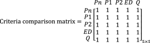 (15)
(15)Using the geometric mean method for each row and then normalizing, the criteria weighting matrix is calculated as follows.
$$ {\text{Criteria}}\,{\text{weighting}}\,{\text{matrix }} = \left[ {\begin{array}{*{20}c} {0.2} \\ {0.2} \\ {0.2} \\ {0.2} \\ {0.2} \\ \end{array} } \right]_{5 \times 1} $$(16) -
Step 4 The ranking matrix is calculated by multiplying the scores matrix in the weighting matrix of criteria (see Eq. (17)).
$$ \left[ {\text{Ranking }} \right]_{45 \times 1} \,(\% ) = \left[ {\text{Scores}} \right]_{45 \times 5} \times \left[ {{\text{Criteria}}\,{\text{weighting}}} \right]_{5 \times 1} \times 100 $$(17) -
Step 5 Finally, the consistency ratio (CR) of the paired comparison matrix should be computed by calculating the consistency index (CI) and the random index (RI). Given that there are five paired comparison matrices, therefore, five consistency ratios must be calculated.
$$ CR = \frac{CI}{RI}. \,Subjected\,to\,CI = \frac{{\lambda_{max} - {\text{m}}}}{m - 1} $$(18)where \( \lambda_{max} \) is the maximum eigenvalue of the paired comparison matrix, m is the size of comparison matrix. RI is related to the size of matrix and is 1.5976 (Donegan and Dodd 1991). The consistency ratio should be less than 0.1. If the consistency ratio exceeds the permissible limit, the AHP responses are not reliable (Donegan and Dodd 1991; Alonso and Lamata 2006).


According to the proposed AHP method, the rank of models is evaluated and presented in Fig. 20. The results illustrated that the models with 2.0 aspect ratio and 8 mm plate thickness have the best-ranking in comparison to other models. As shown, the M2c8 (proposed optimized model by Bagherinejad and Haghollahi 2018) and M1c8 (the proposed optimized model in this study) have the best ranking, respectively (M2c8 = 2.83% and M1c8 = 2.72%). To determine the best form, the sum of rankings for all models of a given form is computed and shown in Fig. 21. It can be seen that the optimized form by the strain energy (M1 models = 22.07%) has the best rank. The optimized perforated plate by the reaction force (M2 models = 20.67%) has the second rank. Also, the results prove that the perforated plate with a central circular hole has a better score (M3 models = 19.36%) in comparison to the multi-circular perforated plates (M4 models = 19.06% and M5 models = 18.84%).

Ranking the models by AHP

Ranking the forms of perforated plates by AHP
The consistency ratios of the five paired comparison matrices are indicated in Table 5. As shown, the values of CR for five paired comparison matrices are less than 0.1.
6 Conclusion
In this paper, topology optimization (TO) was applied to find an optimized perforated plate for various aspect ratios and plate thicknesses. The maximization of strain energy was selected as the objective function. The results of TO showed the plate thickness has no effect on the optimization. The optimized forms for 1.0, 1.5 and 2.0 aspect ratios followed a similar pattern.
The results of TO were compared with the conducted study about the TO of PSPSWs based on the maximization of reaction forces. The comparison illustrated that the results of TO by the strain energy and reaction force are similar for the 0.67 aspect ratio and an X-shaped form was obtained as the optimized form. But, for 1.0, 1.5 and 2.0 aspect ratios, the results of TO by the strain energy were completely different from the TO by the reaction force.
For evaluating the performance of the optimized perforated plates, they were compared with the previous optimized form and other traditional forms. The comparison was done in terms of strength (Pn, P1 and P2), energy dissipation (ED) and fracture tendency (PEEQ). The results of the nonlinear analysis proved that the optimized models based on the strain energy (M1 models) have more significant ductility and flexibility in comparison to the optimized models based on the reaction force (M2 models) and also other traditional models (M3, M4 and M5 models). In contrast, the M2 models have more considerable strength and stiffness in comparison to other models.
Due to the large volume of results, the AHP method was applied to determine the best form. The perforated forms were ranked by AHP. The sum rank of optimized form by the strain energy was 22.07%, while the sum rank of the optimized plate by the reaction force was 20.67%. The ranks of three traditional forms were 19.36%, 19.06% and 18.84%, respectively. The AHP proved that the models with the thick plate (8 mm) and 2.0 aspect ratio have better cyclic behavior. The results of AHP also illustrated that the use of the central circular perforated plate is preferable to the multi-circular perforated plates.
References
ABAQUS. (2014). Analysis user’s manual (V.6-14 ed.). Providence, RI: Dassault Systèmes Simulia.
Alavi, E., & Nateghi, F. (2013a). Experimental study of diagonally stiffened steel plate shear walls. Journal of Constructional Steel Research,139(11), 1795–1811. https://doi.org/10.1061/(ASCE)ST.1943-541X.0000750.
Alavi, E., & Nateghi, F. (2013b). Experimental study on diagonally stiffened steel plate shear walls with central perforation. Journal of Constructional Steel Research,89, 9–20. https://doi.org/10.1016/j.jcsr.2013.06.005.
Allahdadian, S., & Boroomand, B. (2016). Topology optimization of planar frames under seismic loads induced by actual and artificial earthquake records. Engineering Structures,115, 140–154. https://doi.org/10.1016/j.engstruct.2016.02.022.
Alonso, J. A., & Lamata, M. T. (2006). Consistency in the analytic hierarchy process: A new approach. International Journal of Uncertainty, Fuzziness and Knowledge-Based Systems,14(04), 445–459. https://doi.org/10.1142/S0218488506004114.
ATC24. (1992). Guidelines for cyclic seismic testing of components of steel structures for buildings. Redwood City, CA: Applied Technology Council.
Bagherinejad, M. H., & Haghollahi, A. (2018). Topology optimization of steel plate shear walls in the moment frames. Steel and Composite Structures,29(6), 767–779. https://doi.org/10.12989/scs.2018.29.6.771.
Bagherinejad, M. H., & Haghollahi, A. (2019). Topology optimization of perforated steel plate shear walls with thick plate in simple frames. International Journal of Optimization in Civil Engineering,9(3), 457–482.
Bahrebar, M., Kabir, M. Z., Hajsadeghi, M., Zirakian, T., & Lim, J. B. (2016). Structural performance of steel plate shear walls with trapezoidal corrugations and centrally-placed square perforations. International Journal of Steel Structures,16(3), 845–855. https://doi.org/10.1007/s13296-015-0116-y.
Bendsøe, M., & Sigmund, O. (2003). Topology optimization: Theory, methods, and applications (2nd ed.). New York, NY: Springer.
Bhowmick, A. K., Grondin, G. Y., & Driver, R. G. (2014). Nonlinear seismic analysis of perforated steel plate shear walls. Journal of Constructional Steel Research,94, 103–113. https://doi.org/10.1016/j.jcsr.2013.11.006.
Bhushan, N., & Rai, K. (2007). Strategic decision making: Applying the analytic hierarchy process. New York, NY: Springer.
Chan, R., Albermani, F., & Kitipornchai, S. (2011). Stiffness and strength of perforated steel plate shear wall. Procedia Engineering,14, 675–679. https://doi.org/10.1016/j.proeng.2011.07.086.
Dienemann, R., Schumacher, A., & Fiebig, S. (2017). Topology optimization for finding shell structures manufactured by deep drawing. Structural and Multidisciplinary Optimization,56(2), 473–485. https://doi.org/10.1007/s00158-017-1661-0.
Doan, Q. H., & Lee, D. (2019). Optimal formation assessment of multi-layered ground retrofit with arch-grid units considering buckling load factor. International Journal of Steel Structures,19(1), 269–282. https://doi.org/10.1007/s13296-018-0115-x.
Donegan, H., & Dodd, F. (1991). A note on Saaty’s random indexes. Mathematical and Computer Modelling,15(10), 135–137. https://doi.org/10.1016/0895-7177(91)90098-R.
Du, P., Cao, Z., & Fan, F. (2016). Developing of steel plate shear walls braced with slidable multiple X-shaped restrainers: Hysteretic analyses and design recommendations. International Journal of Steel Structures,16(4), 1227–1238. https://doi.org/10.1007/s13296-016-0063-2.
FEMA450. (2003). NEHRP recommended provisions and commentary for seismic regulations for new buildings and other structures. Washington, DC: Federal Emergency Management Agency.
Feng, R.-Q., Liu, F.-C., Xu, W.-J., Ma, M., & Liu, Y. (2016). Topology optimization method of lattice structures based on a genetic algorithm. International Journal of Steel Structures,16(3), 743–753. https://doi.org/10.1007/s13296-015-0208-8.
Formisano, A., Lombardi, L., & Mazzolani, F. M. (2016). Perforated metal shear panels as bracing devices of seismic-resistant structures. Journal of Constructional Steel Research,126, 37–49. https://doi.org/10.1016/j.jcsr.2016.07.006.
Fukada, Y., Minagawa, H., Nakazato, C., & Nagatani, T. (2018). Response of shape optimization of thin-walled curved beam and rib formation from unstable structure growth in optimization. Structural and Multidisciplinary Optimization. https://doi.org/10.1007/s00158-018-1999-y.
Gholizadeh, S., & Poorhoseini, H. (2016). Seismic layout optimization of steel braced frames by an improved dolphin echolocation algorithm. Structural and Multidisciplinary Optimization,54(4), 1011–1029. https://doi.org/10.1007/s00158-016-1461-y.
Jansseune, A., & Corte, W. D. (2017). The influence of convoy loading on the optimized topology of railway bridges. Structural Engineering and Mechanics,64(1), 45–58. https://doi.org/10.12989/sem.2017.64.1.045.
Jia, Z., Ringsberg, J. W., & Jia, J. (2009). Numerical analysis of nonlinear dynamic structural behaviour of ice-loaded side-shell structures. International Journal of Steel Structures,9(3), 219–230. https://doi.org/10.1007/BF03249496.
Kabus, S., & Pedersen, C. B. W. (2012). Optimal bearing housing designing using topology optimization. Journal of Tribology,134(2), 1–9. https://doi.org/10.1115/1.4005951.
Khatibinia, M., & Khosravi, S. (2014). A hybrid approach based on an improved gravitational search algorithm and orthogonal crossover for optimal shape design of concrete gravity dams. Applied Soft Computing,16, 223–233. https://doi.org/10.1016/j.asoc.2013.12.008.
Khatibinia, M., & Naseralavi, S. S. (2014). Truss optimization on shape and sizing with frequency constraints based on orthogonal multi-gravitational search algorithm. Journal of Sound and Vibration,333(24), 6349–6369. https://doi.org/10.1016/j.jsv.2014.07.027.
Khatibinia, M., & Yazdani, H. (2018). Accelerated multi-gravitational search algorithm for size optimization of truss structures. Swarm and Evolutionary Computation,38, 109–119. https://doi.org/10.1016/j.swevo.2017.07.001.
Kutyłowski, R., & Rasiak, B. (2014). Application of topology optimization to bridge girder design. Structural Engineering and Mechanics,51(1), 39–66. https://doi.org/10.12989/sem.2014.51.1.039.
Lee, S., & Tovar, A. (2014). Outrigger placement in tall buildings using topology optimization. Engineering Structures,74, 122–129. https://doi.org/10.1016/j.engstruct.2014.05.019.
Lu, X., Xu, J., Zhang, H., & Wei, P. (2017). Topology optimization of the photovoltaic panel connector in high-rise buildings. Structural Engineering and Mechanics,62(4), 465–475. https://doi.org/10.12989/sem.2017.62.4.465.
Ma, H., Wang, J., Lu, Y., & Guo, Y. (2018). Lightweight design of turnover frame of bridge detection vehicle using topology and thickness optimization. Structural and Multidisciplinary Optimization,59(3), 1007–1019. https://doi.org/10.1007/s00158-018-2113-1.
Mahani, A. S., Shojaee, S., Salajegheh, E., & Khatibinia, M. (2015). Hybridizing two-stage meta-heuristic optimization model with weighted least squares support vector machine for optimal shape of double-arch dams. Applied Soft Computing,27, 205–218. https://doi.org/10.1016/j.asoc.2014.11.014.
Matteis, G. D., Sarracco, G., & Brando, G. (2016). Experimental tests and optimization rules for steel perforated shear panels. Journal of Constructional Steel Research,123, 41–52. https://doi.org/10.1016/j.jcsr.2016.04.025.
Mustafa, M. A., Osman, S. A., Husam, O. A., & Al-Zand, A. W. (2018). Numerical study of the cyclic behavior of steel plate shear wall systems (SPSWs) with differently shaped openings. Steel and Composite Structures,26(3), 361–373. https://doi.org/10.12989/scs.2018.26.3.361.
Purba, R., Bruneau, M., & ASCE, F. (2009). Finite-element investigation and design recommendations for perforated steel plate shear walls. Journal of Structural Engineering,135(11), 1367–1376. https://doi.org/10.1061/(ASCE)ST.1943-541X.0000061.
Qiao, S., Han, X., Zhou, K., & Ji, J. (2016). Seismic analysis of steel structure with brace configuration using topology optimization. Steel and Composite Structures,21(3), 501–515. https://doi.org/10.12989/scs.2016.21.3.501.
Robert, T. M., & Ghomi, S. S. (1992). Hysteretic characteristics of unstiffened perforated steel plate shear panels. Thin-Walled Structures,14(2), 139–151. https://doi.org/10.1016/0263-8231(92)90047-Z.
Roodsarabi, M., Khatibinia, M., & Sarafrazi, S. R. (2016). Hybrid of topological derivative-based level set method and isogeometric analysis for structural topology optimization. Steel and Composite Structures,21(6), 1389–1410. https://doi.org/10.12989/scs.2016.21.6.1389.
Sahoo, D. R., Sidhu, B. S., & Kumar, A. (2015). Behavior of unstiffened steel plate shear wall with simple beam-to-column connections and flexible boundary elements. International Journal of Steel Structures,15(1), 75–87. https://doi.org/10.1007/s13296-015-3005-5.
Søndergaard, M. B., & Pedersen, C. B. W. (2014). Applied topology optimization of vibro-acoustic hearing instrument models. Journal of Sound and Vibration,333(3), 683–692. https://doi.org/10.1016/j.jsv.2013.09.029.
Stromberg, L. L., Beghini, A., Baker, W. F., & Paulino, G. H. (2012). Topology optimization for braced frames: Combining continuum and beam/column elements. Engineering Structures,37, 106–124. https://doi.org/10.1016/j.engstruct.2011.12.034.
Suksuwan, A., & Spence, S. M. J. (2018). Performance-based multi-hazard topology optimization of wind and seismically excited structural systems. Engineering Structures,172, 573–588. https://doi.org/10.1016/j.engstruct.2018.06.039.
Tang, J., Xie, Y. M., & Felicetti, P. (2014). Conceptual design of buildings subjected to wind load by using topology optimization. Wind and Structures,18(1), 021–035. https://doi.org/10.12989/was.2014.18.1.021.
Tomei, V., Imbimbo, M., & Mele, E. (2018). Optimization of structural patterns for tall buildings: The case of diagrid. Engineering Structures,171, 280–297. https://doi.org/10.1016/j.engstruct.2018.05.043.
TOSCA. (2013). Tosca structure documentation (V.8.0 ed.). Karlsruhe: Dassault Systèmes Company.
Tsavdaridis, K. D., Efthymiou, E., Adugu, A., Hughes, J. A., & Grekavicius, L. (2019). Application of structural topology optimisation in aluminium cross-sectional design. Thin-Walled Structures,139, 372–388. https://doi.org/10.1016/j.tws.2019.02.038.
Tsavdaridis, K. D., Kingman, J. J., & Toropov, V. V. (2015). Application of structural topology optimisation to perforated steel beams. Computers & Structures,158, 108–123. https://doi.org/10.1016/j.compstruc.2015.05.004.
Valizadeh, H., Sheidaii, M., & Showkati, H. (2012). Experimental investigation on cyclic behavior of perforated steel plate shear walls. Journal of Constructional Steel Research,70, 308–316. https://doi.org/10.1016/j.jcsr.2011.09.016.
Van Truong, T., Kureemun, U., Tan, V. B. C., & Lee, H. P. (2018). Study on the structural optimization of a flapping wing micro air vehicle. Structural and Multidisciplinary Optimization,57(2), 653–664. https://doi.org/10.1007/s00158-017-1772-7.
Vian, D., Bruneau, M., Tsai, K. C., & Lin, Y. C. (2009). Special perforated steel plate shear walls with reduced beam section anchor beams. I: Experimental investigation. Journal of Structural Engineering,135(3), 211–220. https://doi.org/10.1061/(ASCE)0733-9445(2009)135:3(211).
Wang, M., Yang, W., Shi, Y., & Xu, J. (2015). Seismic behaviors of steel plate shear wall structures with construction details and materials. Journal of Constructional Steel Research,107, 194–210. https://doi.org/10.1016/j.jcsr.2015.01.007.
Wu, Q., Zhou, Q., Xiong, X., & Zhang, R. (2017). Layout and sizing optimization of discrete truss based on continuum. International Journal of Steel Structures,17(1), 43–51. https://doi.org/10.1007/s13296-016-0033-8.
Zehsaz, M., Tahami, F. V., & Akhani, H. (2016). Experimental determination of material parameters using stabilized cycle tests to predict thermal ratchetting. UPB Scientific Bulletin, Series D: Mechanical Engineering,78(2), 17–30.
Zhao, X., Liu, Y., Hua, L., & Mao, H. (2016). Finite element analysis and topology optimization of a 12000KN fine blanking press frame. Structural and Multidisciplinary Optimization,54(2), 375–389. https://doi.org/10.1007/s00158-016-1407-4.
Zhiyi, Y., Kemin, Z., & Shengfang, Q. (2018). Topology optimization of reinforced concrete structure using composite truss-like model. Structural Engineering and Mechanics,67(1), 79–85. https://doi.org/10.12989/sem.2018.67.1.079.
Author information
Authors and Affiliations
Corresponding author
Additional information
Publisher's Note
Springer Nature remains neutral with regard to jurisdictional claims in published maps and institutional affiliations.
Appendix
Appendix
Herein, the values of maximum reaction force during cyclic loading (Pn), maximum reaction force in the last cycle (P1) and the reaction force near the displacement zero in the last cycle (P2) are presented in Table 6. Also, the values of the total energy dissipation due to plastic deformations (ED) and fracture tendency or equivalent plastic strain (PEEQ) at the end of loading are indicated in Table 7.
Rights and permissions
About this article

Cite this article
Bagherinejad, M.H., Haghollahi, A. Study on Topology Optimization of Perforated Steel Plate Shear Walls in Moment Frame Based on Strain Energy. Int J Steel Struct 20, 1420–1438 (2020). https://doi.org/10.1007/s13296-020-00373-x
Received:
Accepted:
Published:
Issue Date:
DOI: https://doi.org/10.1007/s13296-020-00373-x