Hyperbolicity of Moduli Spaces of Log-Canonically Polarized Manifolds

Abstract

In recent years, there are quite a lot of interests and results related to hyperbolicity properties of the base spaces of various families of projective algebraic varieties. Not much is known for families of higher dimensional quasi-projective varieties. The goal of this paper is address the problem for the case of an effectively parametrized family of log-canonically polarized manifolds. We construct a Finsler metric on the base manifold of such a family with the property that its holomorphic sectional curvature is bounded from above by a negative constant, and as a consequence, we deduce the Kobayashi hyperbolicity of the base manifold. The method relies on developing analytic tools to investigate geometry of families of quasi-projective manifolds equipped with Kähler–Einstein metrics, which leads to an appropriate modification of the Weil–Petersson metric on the base manifold.

1 Introduction

1.1 .

The study of the curvature properties of intrinsic metrics on moduli spaces has long been an interesting problem from both differential geometric and algebraic geometric point of view. In particular, people have been interested in the curvature properties of the Weil–Petersson metric. A classical result along this direction is that the Weil–Petersson metric on the moduli space of compact Riemann surfaces of genus $g\ge 2$ is of holomorphic sectional curvature bounded above by some negative constant, which can be traced to the works of Ahlfors ([1, 2]), Royden ([16]) and Wolpert ([26]). Since non-compact Riemann surfaces of finite invariant volume appear naturally in various geometric contexts, it is natural to make similar study for families of punctured Riemann surfaces. Indeed, similar result also holds for the moduli spaces of punctured Riemann surfaces, and this involves a study of harmonic Beltrami differentials with growth conditions near the punctures (see e.g. [20] and the references therein).

In higher dimensional situations, analogous study of the moduli spaces of compact Kähler–Einstein manifolds of negative Ricci curvature from a metric point of view started with the pioneering work of Siu in [18]. A Finsler metric (known as an augmented Weil-Petersson metric in [22]) with negative holomorphic sectional curvature on such a moduli space was eventually found in [21]. Similar to the case of Riemann surfaces, a natural question is whether similar result also holds for the moduli spaces of analogous non-compact manifolds, and in particular, those of certain quasi-projective manifolds of log-general type, which are of interest to complex and algebraic geometers. In fact, this question was raised by several colleagues during the presentation of our work in [21]. In the language of algebraic geometry, this problem can be phrased in terms of a family of pairs $(\overline{M}_t, D_t)$ over a base space S, where $D_t$ is an appropriate divisor in a projective manifold $\overline{M}_t$ for $t\in S$. Our goal in this paper is to address this question for the moduli spaces of certain quasi-projective manifolds equipped with complete Kähler–Einstein metrics of negative Ricci curvature. Existence results of such metrics on quasi-projective manifolds with certain numerical properties would be recalled in Sect. 2.

Our main result in this article is as follows:

Theorem 1

Let $\pi :\mathcal {X}\rightarrow S$ be an effectively parametrized holomorphic family of log-canonically polarized complex manifolds over a complex manifold S. Then, S admits a $C^\infty$ $\text {Aut}(\pi )$-invariant augmented Weil–Petersson metric whose holomorphic sectional curvature is bounded above by a negative constant. As a consequence, S is Kobayashi hyperbolic.

The result is a generalization of the corresponding classical result on moduli of punctured Riemann surface mentioned earlier. We refer the reader to Sect. 2 and Sect. 6 for the definitions of the various terms in Theorem 1. Apart from the result of hyperbolicity mentioned in Theorem 1, another purpose of this paper is to develop and illustrate techniques to handle some difficulties encountered in studying $L^2$ or integrable properties of tensors on non-compact manifolds. The main contribution of the article lies in developing the machinery needed to handle difficulties faced with families of non-compact manifolds as outlined in the next paragraph. Once this is achieved, the formalism of [21] is generalized to our current situation. Our formulation depends on the existence of complete Kähler–Einstein metrics on quasi-projective manifolds, which can be found in [11, 13, 19, 27] and the references therein. In particular, Theorem 1 utilizes the settings in [27] and [11]. The theorem is not stated in its optimal form. For example, the reader will observe that the method here applies to a more general family of quasi-projective manifolds as long as each fiber supports a complete Kähler–Einstein metric of negative scalar curvature and the conditions in Remark 4 are satisfied.

1.2 .

Our approach is to adapt the methods in [21] (which treated the case when the fiber manifolds are compact) to the current situation where the fiber manifolds are non-compact (albeit still endowed with complete Kähler–Einstein metrics of negative Ricci curvature). There are two main obstacles that we need to overcome. The first is to formulate the problem in a correct setting so that one can take care of the issues (arising from non-compactness of the fibers $M_t$’s) in the arguments involving integration by parts. Hence formulation is part of the problem itself. The difficulty is illustrated by the well-known fact that in general, the tensor products of $L^2$ expressions are no longer $L^2$. In our situation, we have to consider various tensor products of the Kodaira–Spencer representatives involved. We need to make sure that all the integrands involved are all integrable. The second is related to the fact that we need to take harmonic projections of various tensor at different stages and sometimes study potentials of $\overline{\partial }$-closed expressions. Again, integrability is an issue. In particular, we have to make sure that we have the desired Hodge decomposition in the current non-compact setting so that Green’s kernels for differential forms on each fiber $M_t$ exist and have sufficient regularity with respect to $t\in S$. Furthermore, we need to prove that the Lie derivatives with respect to the base tangent vectors of the moduli for some integrable tensors are still integrable. This requires getting back to the basic formulations in Hodge theory.

1.3 .

The layout of this article is as follows. In Sect. 2, we collect some background information about Kähler–Einstein metrics of negative Ricci curvature on quasi-projective manifolds and the Kodaira–Spencer deformation theory for such manifolds, and describe the growth conditions for such metrics and the harmonic Kodaira–Spencer tensors involved. In Sect. 3, we give a discussion of the Hodge decomposition on bundle-valued forms on quasi-projective manifolds; in particular, we give a proof that for the family of manifolds under consideration, the Hodge decomposition varies in a smooth manner as the manifold deforms, and that the relevant expressions involved are integrable. Finally, we apply these technical results in a crucial manner to show that the arguments of [21] can be adapted to give a proof of Theorem 1, which forms the bulk of Sects. 4–6.

2 Complete Kähler–Einstein Manifolds and Their Moduli Spaces

2.1 .

Let $M=\overline{M}\setminus D$ be an n-dimensional quasi-projective manifold, where $\overline{M}$ is a projective algebraic manifold, and D is a divisor on $\overline{M}$ with simple normal crossings (meaning that $D=\sum _{i=1}^\ell D_i$ with the irreducible components $D_i$’s being smooth and intersecting transversely). For each $r>0$, we denote by $\Delta _r:=\{z\in \mathbb {C}\,\big |\, |z|<r\}$ (resp. $\Delta ^*_r:=\Delta _r\setminus \{0\}$) the disk (resp. punctured disk) in $\mathbb C$ of radius r and centered at the origin $z=0$. When $r=1$, we simply write $\Delta :=\Delta _1$ and $\Delta ^*:=\Delta ^*_1$. It is well-known that we may cover $\overline{M}$ by a finite collection of coordinate open sets of the form $\Delta ^n$, whose restrictions to M give rise to a finite open cover $\mathcal {U}:=\{U\}$ of M consisting of coordinate open sets of the form

$$\begin{aligned} U=(\Delta ^*)^{k}\times \Delta ^{n-k} \end{aligned}$$

(2.1)

(so that $U=\Delta ^n\cap M$ and $\Delta ^n\cap D$ consists of the union of k coordinate hyperplanes), where $0\leqslant k\leqslant n$. Furthermore, one may assume that M is also covered by the refinement of $\mathcal {U}$ given by $\{U_{\frac{1}{2}}\,\big |\, U\in \mathcal {U}\}$, where we let $U_{r}:=(\Delta ^*_{r})^{k}\times \Delta ^{n-k}_r$ for each $U=(\Delta ^*)^{k}\times \Delta ^{n-k}\in \mathcal {U}$ and each r satisfying $0<r<1$. Let $U=(\Delta ^*)^{k}\times \Delta ^{n-k}$ be as above. Then, the product metric $g_{P,U}$ on U induced by Poincaré metric on each factor of U has its Kähler form given by

$$\begin{aligned} \omega _{P,U}:=\sum _{\alpha =1}^k\frac{\sqrt{-1}\,dz^\alpha \wedge d\overline{z}^\alpha }{|z^\alpha |^2|\log |z^\alpha |^2|^2}+ \sum _{\alpha =k+1}^n\frac{\sqrt{-1}\,dz^\alpha \wedge d\overline{z}^\alpha }{ (1-|z^\alpha |^2)^2}. \end{aligned}$$

(2.2)

Here, for each $1\le \alpha \le n$, $z^\alpha$ denotes the Euclidean coordinate on $\alpha$-th factor of U. A complete Kähler metric g on $M=\overline{M}\backslash D$ is said to have Poincaré growth near D if for some (and hence all) open coordinate cover $\mathcal {U}=\{U\}$ as described above and each $U\in \mathcal {U}$, the restriction $g\vert _{U_{\frac{1}{2}}}$ is quasi-isometric to $g_{P,U}\vert _{U_{\frac{1}{2}}}$ on $U_{\frac{1}{2}}$. Here we recall that two metrics $g_1$ and $g_2$ on a manifold X are said to be quasi-isometric to each other if there exists a constant $C>0$ such that $\dfrac{1}{C} g_2\leqslant g_1 \leqslant C g_2$ on X.

2.2 .

Next, we recall the following definition similar to the one used in [13, 19, 23, 27] and [11]:

Definition 1

We say that a complete Kähler metric g on a non-compact complex manifold M has bounded geometry if

• (a) The curvature tensor of g is bounded on M, and

• (b) the volume of (M, g) is finite.

Let $\overline{M}$ be a projective manifold, and let $D=\sum _{i=1}^\ell D_i$ be a divisor on $\overline{M}$ with simple normal crossings. As usual, we will denote by [D] (resp. $[D_i]$) the divisor line bundle on $\overline{M}$ associated to D (resp. $[D_i]$), so that $[D]=\sum _{i=1}^\ell [D_i]$ when the tensor product of line bundles is written additively. When a holomorphic line bundle L is ample, we simply write $L>0$. More generally, for an $\mathbb {R}$-divisor $\nu$ on $\overline{M}$, we write $\nu >0$ if its class in $H^{1,1}(\overline{M},\mathbb {R})$ is represented by a positive d-closed (1, 1)-form on $\overline{M}$.

Definition 2

We say that a non-compact complex manifold M is log-canonically polarized if there exist a projective manifold $\overline{M}$ and a divisor $D=\sum _{i=1}^\ell D_i$ on $\overline{M}$ with simple normal crossings such that M is biholomorphic to $\overline{M}\setminus D$, and the following two conditions are satisfied:

• (i) $K_{\overline{M}}+\sum _{i=1}^\ell \alpha _i D_i>0$ on $\overline{M}$ for some $\alpha _1,\cdots ,\alpha _\ell \in \mathbb {R}$ satisfying $-\infty <\alpha _i\le 1$, $i=1,\cdots ,\ell$, and

• (ii) $(K_{\overline{M}}+D)\big |_{D_i}>0$ on $D_i$ for each smooth irreducible component $D_i$ of D.

Remark 1

In the case when D is smooth and irreducible (so that $\ell =1$), a pair $(\overline{M},D)$ satisfying (i) with $\alpha _1=1$ (so that (ii) is also satisfied) is called a framed manifold of type (N) in [17].

2.3 .

We recall the following result of Wu:

Proposition 1

([27, Theorem 1.2]) Suppose a quasi-projective manifold $M=\overline{M}\setminus D$ is log-canonically polarized (cf. Definition 2). Then, a complete Kähler–Einstein metric with negative Ricci curvature and bounded geometry exists on M. Furthermore, the Kähler–Einstein metric has Poincaré growth near the divisor D.

Remark 2

• (i) It follows from Yau’s Schwarz lemma [28] that the complete Kähler–Einstein metric in Proposition 1 is unique up to a positive constant multiple (resp. unique if the constant Ricci curvature is normalized to be a fixed negative number).

• (ii) Proposition 1 for the case when D is smooth and irreducible was due to Tian-Yau [19].

• (iii) Suppose M is a non-compact complex manifold equipped with a complete Kähler–Einstein metric of negative Ricci curvature and bounded geometry. Then, one knows that there exist a projective algebraic manifold $\overline{M}$ and a divisor D on $\overline{M}$ with simple normal crossings such that $M\cong \overline{M}\setminus D$ (cf. [15, 29]).

2.4 .

We recall the deformation of quasi-projective manifolds and the associated Kodaira–Spencer map in our setting. A quasi-projective manifold M can be written as a pair $(\overline{M},D)$ so that $M=\overline{M}\setminus D$, where $\overline{M}$ is a projective manifold, and D is a divisor in $\overline{M}$ with simple normal crossings. As such, we will consider the deformations of M that will correspond to deformations of the pair $(\overline{M},D)$, or in other words, the deformations of $\overline{M}$ which fix D. Consider $\Omega _{\overline{M}}(\log D)^\vee :=T_{\overline{M}}(\log D)$, which is the subsheaf of $T_{\overline{M}}$ consisting of holomorphic tangent vector fields which map the ideal sheaf of D into itself. Then, the Kodaira–Spencer map associated to such deformations takes values in $H^1(\overline{M}, \Omega _{\overline{M}} (\log D)^\vee )$. We refer the reader to [12] for more details on deformation of quasi-projective manifolds.

A family of n-dimensional quasi-projective manifolds $\pi :\mathcal {X}\rightarrow S$ over a complex manifold S means that $\pi$ is a surjective holomorphic map of maximal rank between two complex manifolds $\mathcal {X}$ and S, and for each $t\in S$, the fiber $M_t:=\pi ^{-1}(t)$ is an n-dimensional quasi-projective manifold; furthermore, we will always assume that there exists a family of projective manifolds $\overline{\pi }:\overline{\mathcal {X}}\rightarrow S$ and a divisor D on $\overline{\mathcal {X}}$ such that $\mathcal {X}= \overline{\mathcal {X}}\setminus D$, and for each $t\in S$, ${\overline{M}}_t:=\overline{\pi }^{-1}(t)$ is a projective manifold, $D_t:=\overline{\pi }^{-1}(t)\cap D$ is a divisor in ${\overline{M}}_t$ with simple normal crossings (so that $M_t$ is realized as the pair $({\overline{M}}_t, D_t)$). As mentioned earlier, we will only consider those families of quasi-projective manifolds for which the Kodaira–Spencer map takes values in $H^1(\overline{M}_t, \Omega _{\overline{M}_t} (\log D_t)^\vee )$ for each $t\in S$. Recall that a family of quasi-projective manifolds $\pi :\mathcal {X}\rightarrow S$ as above is said to be effectively parametrized if the Kodaira–Spencer map $\rho _t : T_tS \rightarrow H^1(\overline{M}_t, \Omega _{\overline{M}_t} (\log D_t)^\vee )$ is injective for each $t \in S$. A family of log-canonically polarized manifolds is defined as a family of quasi-projective manifolds $\pi :\mathcal {X}\rightarrow S$ such that each fiber $M_t=\pi ^{-1}(t)$, $t\in S$, is log-canonically polarized.

Let $\pi :\mathcal {X}\rightarrow S$ be an effectively parametrized family of log-canonically polarized manifolds. Then, as quoted in Proposition 1, each fiber $M_t=\pi ^{-1}(t)$ admits a complete Kähler–Einstein metric g(t) with negative Ricci curvature $k<0$. It is easy to see that k can be chosen to be independent of $t\in S$, and with such a choice of k, g(t) is uniquely determined (cf. Remark 2 (i)). Upon following an argument similar to case of families of framed manifolds in [17, Section 2], one sees that g(t) varies smoothly in $t\in S$. Denote the Kähler form of g(t) by $\omega (t)$, and consider the relative canonical line bundle on $\mathcal {X}$ given by $K_{\mathcal {X}\big |S}:=K_{\mathcal {X}}\otimes (\pi ^*K_S)^{-1}$. Then as in the compact case, the volume forms associated to the $\omega (t)$’s define a Hermitian metric $\lambda$ on $K_{\mathcal {X}\big |S}^{-1}$, and one obtains a d-closed (1, 1)-form on $\mathcal {X}$ given by

$$\begin{aligned} \omega _{\mathcal {X}}:=\dfrac{2\pi }{k}c_1\left( K_{\mathcal {X}\big |S}^{-1},\lambda \right) \quad \text {so that }\omega _{\mathcal {X}}\big |_{M_t}=\omega (t)\text { for all }t\in S. \end{aligned}$$

(2.3)

Throughout this article, we will use $(z,t)=(z^1,\cdots , z^n, t^1,\cdots , t^m)$ to denote local holomorphic coordinate functions on some coordinate open subset of $\mathcal {X}$, so that $\pi$ corresponds to the projection map $(z,t)\rightarrow t$, and $t=(t^1,\cdots , t^m)$ (resp. $z=(z^1,\cdots , z^n)$) forms local holomorphic coordinate functions on some open subset of S (resp. $M_t$). We will index the components of tensors on $M_t$ in the holomorphic tangential directions by Greek letters $\alpha ,\beta ,\gamma$ (with the range $1,\cdots , n$), etc, and those in the complexified tangential directions by lower case Latin letters a, b, c, d (with the range $1,\cdots , n,\overline{1},\cdots ,\overline{n}$), etc. The components of tensors along the base directions will be indexed by the letters i, j (with the range $1,\cdots , m$), etc. We also denote $\partial _\alpha :=\frac{\partial }{\partial z^\alpha }$, and $\partial _i=\frac{\partial }{\partial s^i}$, etc. We write $\omega _\mathcal {X}=\sqrt{-1}\sum _{I,J}g_{I\overline{J}} dw^I\wedge d\overline{w}^J$, where w can be z or t, and the indices I, J can be $\alpha$ or i, etc. In particular, the $g_{\alpha \overline{\beta }}$’s give the components of $\omega (t)$ on $M_t$. Finally, we will adopt the Einstein summation notation for the indices along the fibers $M_t$’s if no confusion arises.

Next, we recall the horizontal lifting of vector fields defined by Schumacher in [17]. For a local tangent vector field u of type (1, 0) on an open subset U of S, the horizontal lifting of u is defined as the unique vector field $v_u$ on $\pi ^{-1}(U)$ of type (1, 0) such that $\pi _*v_u=u$ and $v_u(z,t)$ is orthogonal to $T_zM_t$ with respect to $\omega _\mathcal {X}$ for each $(z,t)\in \pi ^{-1}(U)$. For each $t\in U$, let

$$\begin{aligned} \Phi (u(t)):=\overline{\partial }v_u\big |_{M_t}\in \mathcal {A}^{0,1}_{M_t}(TM_t), \end{aligned}$$

(2.4)

where as usual, $\mathcal {A}^{0,1}_{M_t}(TM_t)$ denotes the set of $C^\infty$ $TM_t$-valued (0, 1)-forms on $M_t$. Then by following the arguments of [17, Section 3], one sees that $\Phi (u(t))$ is the $L^2$ harmonic representative of the Kodaira–Spencer class of $\rho _t(u)$ in $H^1(\overline{M}_t, \Omega _{\overline{M}_t} (\log D_t)^\vee )$ (see also Lemma 1 below for the asymptotic behavior of $\Phi (u(t))$ near $D_t$). For simplicity of notation and as in [21], we will suppress the subscript t in the following discussions when there is no danger of confusion. When $u={\partial }/{\partial t^i}$ is a coordinate vector field, we simply denote its horizontal lifting by $v_i:=v_{\partial /\partial t^i}$ and the associated harmonic Kodaira–Spencer representative by $\Phi _i:=\Phi (\partial /\partial t^i)$. Write $\Phi _i=(\Phi _i)_{\bar{\beta }}^\alpha \frac{\partial }{\partial z^\alpha }\otimes d\bar{z}^\beta$ in terms of local holomorphic coordinates on $M_t$. One easily sees that $v_i$ and the $(\Phi _i)_{\bar{\beta }}^\alpha$’s are given locally by

$$\begin{aligned} v_i&=\partial _i+v_i^\alpha \partial _\alpha ,\quad \text {where } v_i^\alpha :=-g^{\bar{\beta }\alpha }g_{i\bar{\beta }},~\text {and} \end{aligned}$$

(2.5)

$$\begin{aligned} (\Phi _i)_{\bar{\beta }}^\alpha&=\partial _{\bar{\beta }}v_i^\alpha = -\partial _{\bar{\beta }}(g^{\bar{\gamma }\alpha }g_{i\bar{\gamma }}) \end{aligned}$$

(2.6)

Here, $g^{\bar{\beta }\alpha }$ denotes the components of the inverse of $g_{\alpha \bar{\beta }}$

Definition 3

Let $M=\overline{M}\setminus D$ with $D=\sum _{i=1}^\ell D_i$, and $\mathcal {U}:=\{U\}$ be a finite open coordinate cover of M such that the refinement $\{U_{\frac{1}{2}}\,\big |\, U\in \mathcal {U}\}$ also covers M as in §2.1.

• (i) We denote by $\widetilde{\mathcal {A}}^{0,1}(\Omega ^1_{\overline{M}}(\log D)^\vee )$ the set of elements $\varphi$ in $\mathcal {A}_M^{0,1}(TM)$ such that for each $U=(\Delta ^*)^{k}\times \Delta ^{n-k}\in \mathcal {U}$ as in (2.1), $\varphi =\varphi _{\bar{\beta }}^\alpha \frac{\partial }{\partial z^\alpha }\otimes d\bar{z}^\beta$ satisfies the following pointwise estimates on $U_{\frac{1}{2}}=(\Delta ^*_{\frac{1}{2}})^{k}\times \Delta ^{n-k}_{\frac{1}{2}}$:

  $$\begin{aligned} \varphi ^{{\alpha }}_{\overline{\beta }}=\left\{ \begin{array}{cl} O\left( \dfrac{|z^{{\alpha }}||\log |z^{{\alpha }}||}{|z^{\beta }||\log |z^{\beta }||}\right) &{} \text{ for } \ \ {\alpha }\leqslant k, \ \beta \leqslant k, \ {\alpha }\ne \beta ;\\ O(|z^{{\alpha }}||\log |z^{{\alpha }}||)&{} \text{ for } \ \ {\alpha }\leqslant k, \ \beta> k;\\ O\left( \dfrac{1}{|z^{\beta }||\log |z^{\beta }||}\right) &{} \text{ for } \ \ {\alpha }> k, \ \beta \leqslant k;\\ O(1) &{} \text{ for } \ \ {\alpha }=\beta , \text{ or } \ \ {\alpha }> k,\, \beta > k. \end{array}\right. \end{aligned}$$

  (2.7)

• (ii) More generally, for $0\le p,r\le n$, we denote by $\widetilde{\mathcal {A}}^{0,p}(\Omega ^r_{\overline{M}}(\log D)^\vee ))$ the set of elements $\varphi$ in $\mathcal {A}_M^{0,p}(\wedge ^r(TM))$ such that for each $U=(\Delta ^*)^{k}\times \Delta ^{n-k}\in \mathcal {U}$, $\varphi =\varphi _{\overline{\beta _1\cdots \beta _p}}^{\alpha _1\cdots \alpha _r} \frac{\partial }{\partial z^{\alpha _1}}\wedge \cdots \wedge \frac{\partial }{\partial z^{\alpha _r}} \otimes d\overline{z}^{\beta _1}\wedge \cdots \wedge d\overline{ z}^{\beta _p}$ satisfies the following pointwise estimates on $U_{\frac{1}{2}}=(\Delta ^*_{\frac{1}{2}})^{k}\times \Delta ^{n-k}_{\frac{1}{2}}$:

  $$\begin{aligned} \varphi _{\overline{\beta _1\cdots \beta _p}}^{\alpha _1\cdots \alpha _r}=O\big ( \dfrac{\prod _{ \alpha _i\le k} |z^{\alpha _i}||\log |z^{\alpha _i}||}{\prod _{ \beta _j\le k}|z^{\beta _j}||\log |z^{\beta _j}||} \big ) \end{aligned}$$

  (2.8)

  for all $1\le \alpha _1<\cdots <\alpha _r\le n$ and $1\le \beta _1<\cdots <\beta _p\le n$. Here, $\prod _{ \alpha _i\le k} |z^{\alpha _i}||\log |z^{\alpha _i}||$ (resp. $\prod _{ \beta _j\le k}|z^{\beta _j}||\log |z^{\beta _j}||$) is understood to be 1 if $\alpha _i>k$ for all i (resp. $\beta _j>k$ for all j).

One easily sees that the above definition does not depend on the choice of finite open coordinate cover $\mathcal {U}:=\{U\}$ of M (as long as $\{U_{\frac{1}{2}}\,\big |\, U\in \mathcal {U}\}$ still covers M).

Lemma 1

Let $\pi :\mathcal {X}\rightarrow S$ be an effectively parametrized family of log-canonically polarized manifolds with $\pi ^{-1}(t)=M_t=\overline{M_t}\setminus D_t$ and $D_t=\sum _{i=1}^\ell D_{t,i}$ for each $t\in S$. Let u be a local tangent vector field on an open subset W of S, and let $\Phi (u(t))$ be as in (2.4). Then $\Phi (u(t))\in \widetilde{\mathcal {A}}^{0,1}(\Omega _{\overline{M}_t}(\log D_t)^\vee )$ for each $t\in W$. In particular, the $C^0$ norm of $\Phi (u(t))$ (with respect to $g_t$) is finite for each $t\in W$.

Proof

The lemma for the case when $\ell =1$ (i.e., when $D_t$ is smooth and irreducible) was obtained in [17, Lemma 3], and the proof generalizes readily to the case when $\ell >1$, which we describe briefly here. Recall that for each $t\in W\subset S$, the compactifying divisor $D_t=\sum _{i=}^\ell D_{t,i}$ on $\overline{M}_t$ is with simple normal crossings. Without loss of generality, we may assume that $W=\Delta ^m$ is a coordinate open subset of S, and $u(t)=\frac{\partial }{\partial t^i}$ is a coordinate vector field on W. Recall from Proposition 1 and the discussion in the beginning of this section that the family of complete Kähler–Einstein metrics g(t) of negative Ricci curvature on $M_t=\overline{M}_t\setminus D_t$, $t\in S$, constructed in [27, Theorem 1.2] are such that each g(t) has bounded geometry and has Poincaré growth near $D_t$. For each point $t\in W$, let $\mathcal {U}_t:=\{U_t\}$ be a finite open coordinate cover of $M_t$ such that the refinement $\{U_{t,\frac{1}{2}}\,\big |\, U_t\in \mathcal {U}_t\}$ also covers $M_t$ as in 2.1. Then, a quasi-coordinate system in the sense of Tsuji [23] can be introduced on $M_{t}$ near the compactifying divisor $D_{t}$, as described in [27, page 402]. Briefly, for each $U_t=(\Delta ^*)^{k}\times \Delta ^{n-k}\in \mathcal {U}$, a quasi-coordinate system for U is a collection of holomorphic maps $\phi _\eta : (\Delta _{\frac{3}{4}})^{k}\times \Delta ^{n-k}\rightarrow U$ indexed by $\eta =(\eta _1,\cdots ,\eta _k)\in (0,1)^k$ such that each $\phi _\eta$ is a holomorphic covering map from $(\Delta _{\frac{3}{4}})^{k}\times \Delta ^{n-k}$ onto its image $\phi _\eta ((\Delta _{\frac{3}{4}})^{k}\times \Delta ^{n-k})$, $\bigcup _{\eta \in (0,1)^k} \phi _\eta ((\Delta _{\frac{3}{4}})^{k}\times \Delta ^{n-k})=U$, and $\phi _\eta ^*(\omega _{P,U})=\omega _{P,\Delta ^n}\big |_{(\Delta _{\frac{3}{4}})^{k}\times \Delta ^{n-k}}$. Here, $\omega _{P,U}$ is as in (2.2), etc. By following the arguments of Schumacher in [17, Section 3], one easily sees that the metric tensor components $g_{{\alpha }\overline{\beta }}, g_{i\overline{\beta }}$ (cf. (2.5)) and their derivatives are of finite Hölder $C^{k,\lambda }$ norm with respect to the Poincaré metrics in the quasi-coordinates for all $k\in \mathbb {N}$ and $\lambda \in (0,1)$, and the $g_{i\overline{\beta }}$’s vary smoothly with respect to the base coordinate t. Then the statement $\Phi (u(t))\in \widetilde{\mathcal {A}}^{0,1}(\Omega _{\overline{M}_t}(\log D_t)^\vee )$ in Lemma 1 follow from (2.4), (2.5) and (2.6) and straightforward computations as in [17, Section 3]. Finally the finiteness of the $C^0$ norm of $\Phi (u(t))$ with respect to $g_t$ follows readily the facts that $g_t$ has Poincaré growth near $D_t$ and $\Phi (u(t))\in \widetilde{\mathcal {A}}^{0,1}(\Omega _{\overline{M}_t}(\log D_t)^\vee )$. $\square$

Remark 3

Let $\Phi (u(t))$ be as in Lemma 1. Then, Lemma 1 implies readily that $\Phi (u(t))\in \mathcal {A}_{(2)}^{(0,1)}(TM_t)$. Moreover, similar reasoning as in the proof of Lemma 1 leads to $L^2$-integrability of the covariant derivatives of $\Phi (u(t))$ (along the fiber direction) and $L^2$-integrability of the partial derivatives of $\Phi (u(t))$ with respect to the base variable $t\in S$.

Remark 4

Fix a relatively compact coordinate neighborhood $W=\Delta ^m\subset \subset S$ with coordinates $t=(t_1,\cdots , t_m)$. For each $1\le i,j\le m$, let $v_i$, $v_j$ be as in (2.5). Then with respect to $\omega _{\mathcal {X}}$ (cf. (2.3)), one has the pointwise pairing given by

$$\begin{aligned} v_i\cdot \overline{v_{j}}=g_{i\overline{j}}+v^{\alpha }_i\overline{g_{j\overline{\alpha }}}=g_{i\overline{j}}-g_{i\overline{\beta }}g_{\alpha \overline{j}}g^{\overline{\beta }\alpha }. \end{aligned}$$

(2.9)

Together with the description of g(t)’s in the proof of Lemma 1, it follows readily that there exists a positive continuous function $C:U\rightarrow \mathbb {R}$ such that $v_i\cdot \overline{v_{j}}(x)\ge -C(\pi (x))$ for all $x\in \pi ^{-1}(W)$.

3 Remarks About $L^2$ Cohomology

3.1 .

For our ensuing discussion, we need to understand the $L^2$ Hodge decomposition for a family of quasi-projective manifolds equipped with complete Kähler metrics. Due to a lack of suitable literature on such issues, we take up the task of explaining the details in this section.

First, we recall some basic facts about the $L^2$-cohomology on a complete Kähler manifold. We refer the reader to [30] and [6] for the basic settings. The known results are sufficient for us to apply arguments in [21] to the setting of a moduli space of log-canonically polarized manifolds as mentioned in Theorem 1. In particular, it leads to the existence of Green’s kernel as well as spectral decomposition associated to the Laplacian on each fiber manifold.

Let (E, h) be a Hermitian holomorphic vector bundle over a complete non-compact Kähler manifold M, where h denotes the Hermitian metric on the holomorphic vector bundle E. Denote the complete Kähler metric and the associated Kähler form on M by g and $\omega$, respectively. For each $0\le p\le n:={\text{ dim }}_\mathbb {C}M$, we denote by $\mathcal {A}^{0,p}(M, E)$ (resp. $L_{(2)}^{0,p}(M, E)$) the space of smooth (resp. $L^2$) E-valued (0, p)-forms on M. Here, as usual, the $L^2$ inner product on M is given by

$$\begin{aligned} (\phi ,\psi ):=\int _M \langle \phi ,\psi \rangle _{h,g}\dfrac{\omega ^n}{n!}, \end{aligned}$$

(3.1)

where $\langle \phi ,\psi \rangle _{h,g}$ denotes the pointwise inner product of the two E-valued (0, p)-forms $\phi$, $\psi$ on M with respect to h and g, so that $L_{(2)}^{0,p}(M, E)$ denotes the space of E-valued (0, p)-forms $\phi$ such that $\Vert \phi \Vert _2:=\sqrt{(\phi ,\phi )_{(2)}}<\infty$.

Let

$$\begin{aligned} \mathcal {A}_{(2)}^{0,p}(M, E):=\mathcal {A}^{0,p}(M, E)\cap L_{(2)}^{0,p}(M, E), \end{aligned}$$

(3.2)

and let $\text{ Dom }(\overline{\partial }_p):=\{{\alpha }\in \mathcal {A}_{(2)}^{0,p}(M, E)\,\big |\,\overline{\partial }_p{\alpha }\in \mathcal {A}_{(2)}^{0,p+1}(M, E)\}$, where $\overline{\partial }_p:\mathcal {A}^{0,p}(M, E)\rightarrow \mathcal {A}^{0,p+1}(M,E)$ is the usual $\overline{\partial }$ operator on $\mathcal {A}^{0,p}(M, E)$. The $L^2$ Dolbeault cohomology groups are defined to be

$$\begin{aligned} H^p_{(2)}(M, E):=\ker (\overline{\partial }_p)/\text{ Im }(\overline{\partial }_{p-1}),\quad 0\le p\le n. \end{aligned}$$

(3.3)

The operator $\overline{\partial }_p$ has a well-defined strong closure $\widetilde{\overline{\partial }}_p$ in $L^2$. We say that $\widetilde{\overline{\partial }}_p {\alpha }=\beta$ if there exists a sequence ${\alpha }_i\in \text{ Dom }(\overline{\partial }_p)$ such that ${\alpha }_i\rightarrow {\alpha }$ and $\overline{\partial }{\alpha }_i\rightarrow \beta$ in $L^2$. It is well known that there is an isomorphism

$$\begin{aligned} H^p_{(2)}(M, E)\cong \ker (\widetilde{\overline{\partial }}_p)/\text{ Im }(\widetilde{\overline{\partial }}_{p-1}). \end{aligned}$$

(3.4)

From the works of Andreotti–Vesentini [4] and Zucker [30], we know that $\text{ Im }(\widetilde{\overline{\partial }}_{p-1})$ is closed in $\ker (\widetilde{\overline{\partial }}_p)$, and hence $H^p_{(2)}(M, E)$ is the same as the corresponding reduced $L^2$ cohomology, which is defined to be $\ker (\overline{\partial }_p)/\overline{\text{ Im }(\overline{\partial }_{p-1})}$, where ${\overline{\text{ Im }(\overline{\partial }_{p-1})}}$ is defined to be the closure of $\text{ Im }(\overline{\partial }_{p-1})$ in $\ker (\overline{\partial }_p)$. For simplicity, we will denote the $\overline{\partial }_p$’s and the $\widetilde{\overline{\partial }}_p$’s all by $\overline{\partial }$ when no confusion arises. As usual, we denote the $\overline{\partial }$-Laplacian by $\square :=\overline{\partial }\overline{\partial }^{*}+\overline{\partial }^{*}\overline{\partial }$. Let $\mathcal {H}^{(0,p)}_{(2)}(M, E):=\{ \phi \in \mathcal {A}_{(2)}^{0,p}(M, E)\,\big |\, \square \phi =0\}$ be the space of $\square$-harmonic E-valued (0, p)-forms on M. Since M is complete, using cut-off functions as in Gaffney’s trick (cf. [9, 10]), one sees that the usual arguments for Hodge decomposition of differential forms give rise to $L^2$-Hodge decomposition; namely, any $\eta \in \mathcal {A}^{(0,p)}_{(2)}(M, E)$ can be written as

$$\begin{aligned} \eta =H\eta +\square \beta =H\eta +\overline{\partial }\overline{\partial }^*\beta +\overline{\partial }^*\overline{\partial }\beta , \end{aligned}$$

(3.5)

for some $\beta \in L^{(0,p)}_{(2)}(M, E)$, where $H\eta$ is the $L^2$-harmonic projection of $\eta$. The decomposition is orthogonal with respect to the $L^2$ inner product in (3.1), and $H\eta$ is uniquely defined by $\eta$. The choice of $\beta$ in (3.5) is not unique, but is determined uniquely up to an $L^2$ harmonic form. In fact, by applying (3.5) to $\beta$, we have

$$\begin{aligned} \beta =H\beta +\square \lambda \end{aligned}$$

(3.6)

for some $\lambda \in L^{(0,p)}_{(2)}(M, E)$. Define the Green’s operator $G:L^{(0,p)}_{(2)}(M, E)\rightarrow L^{(0,p)}_{(2)}(M, E)$ given by

$$\begin{aligned} G\eta :=\beta -H\beta . \end{aligned}$$

(3.7)

It is easy to see that G is well-defined (i.e. $G\eta$ in (3.7) does not depend on the choice of $\beta$ in (3.6)), and G satisfies

$$\begin{aligned} \eta =H\eta + \square G\eta . \end{aligned}$$

(3.8)

We note that if $\eta \in \ker (\overline{\partial }_p)\cap \mathcal {A}^{(0,p)}_{(2)}(M, E)$ so that $\eta$ is $\overline{\partial }$-closed, then the expression $\overline{\partial }^*\overline{\partial }\beta$ in (3.5) vanishes (since it is orthogonal to the other expressions in (3.5), which are all $\overline{\partial }$-closed). Thus, (3.5) and (3.8) can be written as

$$\begin{aligned} \eta =H\eta +\overline{\partial }_{p-1}\overline{\partial }_p^*\beta =H\eta + \overline{\partial }_{p-1}\overline{\partial }_{p}^*G\eta \quad \text {if }\overline{\partial }\eta =0. \end{aligned}$$

(3.9)

It follows readily that the map $\eta \rightarrow H\eta$ for $\eta \in \ker (\overline{\partial }_p)\cap \mathcal {A}^{(0,p)}_{(2)}(M, E)$ leads to a vector space isomorphism

$$\begin{aligned} H^p_{(2)}(M, E)\cong \mathcal {H}^{(0,p)}_{(2)}(M, E). \end{aligned}$$

(3.10)

The classical approach to Hodge decomposition as above makes use of the regularity of elliptic equations. See also the arguments in 3.2 in which an approach via parabolic equation due to [10, 14] is recalled.

3.2 .

In this subsection, we are going to study the smoothness properties of the $L^2$ Hodge decomposition described in 3.1 in the setting of a family of manifolds. As such, we only need to consider the case when the base manifold S is a polydisk of the form $\Delta _\epsilon ^m$, and we may shrink $\epsilon$ during our discussion, if necessary.

Consider a local family of log-canonically polarized manifolds $\pi :\mathcal {X}\rightarrow \Delta _\epsilon ^m$ as in 2.4. Recall that it arises as the restriction of a family of projective manifolds $\overline{\pi }:\overline{\mathcal {X}}\rightarrow \Delta _\epsilon ^m$, such that $\mathcal {X}= \overline{\mathcal {X}}\setminus D$ for a divisor D on $\overline{\mathcal {X}}$, and for each $t\in \Delta _\epsilon ^m$, $M_t={\pi }^{-1}(t)$ is a log-canonically polarized manifold, ${\overline{M}}_t:=\overline{\pi }^{-1}(t)$ is a projective manifold, $D_t:=\overline{\pi }^{-1}(t)\cap D$ is a divisor in ${\overline{M}}_t$ with simple normal crossings (so that $M_t$ is realized as the pair $({\overline{M}}_t, D_t)$). For simplicity, we will denote the family described above by $\{M_t\}_{t\in \Delta _\epsilon ^m}$ or $\{({\overline{M}}_t, D_t)\}_{t\in \Delta _\epsilon ^m}$. Recall that there exists a smooth family of complete Kähler–Einstein metrics $g_t$ on $M_t$ as obtained in [27] and described in 2.3 and 2.4. It is easy to see that upon shrinking $\epsilon$ if necessary, one can cover $\overline{\mathcal {X}}$ by a finite collection of coordinate open sets of the form $\Delta ^n\times \Delta _\epsilon ^m$ (with $\overline{\pi }\big |_{\Delta ^n\times \Delta _\epsilon ^m}$ given by the projection map onto the second factor $\Delta ^n\times \Delta _\epsilon ^m\rightarrow \Delta _\epsilon ^m$), whose restrictions to $\mathcal {X}$ give rise to a finite open cover $\mathcal {U}:=\{U\}$ of $\mathcal {X}$ consisting of coordinate open sets of the form $U=(\Delta ^*)^{k}\times \Delta ^{n-k}\times \Delta _\epsilon ^m$ (so that $U=(\Delta ^n\times \Delta _\epsilon ^m)\cap \mathcal {X}$ and $(\Delta ^n\times \Delta _\epsilon ^m)\cap D$ consists of the union of k coordinate hyperplanes), where $0\leqslant k\leqslant n$; furthermore, one may assume that $\mathcal {X}$ is also covered by the refinement of $\mathcal {U}$ given by $\{U_{\frac{1}{2}}\,\big |\, U\in \mathcal {U}\}$, where for each $U=(\Delta ^*)^{k}\times \Delta ^{n-k}\times \Delta _\epsilon ^m$, $U_{\frac{1}{2}}$ is given by $(\Delta ^*_{\frac{1}{2}})^{k}\times \Delta ^{n-k}_{\frac{1}{2}}\times \Delta _\epsilon ^m$. For each $t\in \Delta _\epsilon ^m$ and each $U\in \mathcal {U}$, let $U_t:=U\cap \pi ^{-1}(t)$ for each $U\in \mathcal {U}$, and let $\mathcal {U}_{t,\frac{1}{2}}:=U_{\frac{1}{2}}\cap \pi ^{-1}(t)$. Then it is easy to see that for each $t\in \Delta _\epsilon ^m$, $M_t$ is covered by the open coordinate system $\mathcal {U}_t:=\{U_t:U\in \mathcal {U}\}$ (as well as its refinement $\mathcal {U}_{t,\frac{1}{2}}:=\{U_{t,\frac{1}{2}}:U\in \mathcal {U}\}$). By taking relatively compact open subsets of the universal covers of the elements of $\{U\}$ and shrinking $\epsilon$ if necessary, it is easily to see that one can introduce a family of quasi-coordinates of the form $V\times \Delta _\epsilon ^m$, where for each $t\in \Delta _\epsilon ^m$, $V_t:=V\times \{t\}\cong V\subset \mathbb {C}^n$ is a quasi-coordinate for $U_t$ (cf. the proof of Lemma 1). We have

Lemma 2

Let $\{M_t\}_{t\in \Delta _\epsilon ^m}$ be a local family of n-dimensional log-canonically polarized manifolds endowed with a smooth family of complete Kähler–Einstein metrics $g_t$ on $M_t$, $t\in \Delta _\epsilon ^m$, as described above (and in 2.3 and 2.4). Let $(E_t,h_t)$ be a smooth family of Hermitian holomorphic vector bundles on $M_t$, $t\in \Delta _\epsilon ^m$. Let p be an integer satisfying $0\le p\le n$. Suppose that $A_t\in \mathcal {A}_{(2)}^{0,p}(M_t, E_t)$ is a family of (fiberwise) $\overline{\partial }$-closed $L^2$ $E_t$-valued (0, p)-forms on $M_t$ such that $A_t(x)$ is $C^\infty$ with respect to t for $t\in \Delta _\epsilon ^m$. Let $H_tA_t\in \mathcal {H}^{(0,p)}_{(2)}(M_t, E_t)$ be the harmonic projection of $A_t$ for each $t\in \Delta _\epsilon ^m$. Then, the following statements hold:

• (a) One has $H_tA_t\in \mathcal {A}_{(2)}^{0,p}(M_t, E_t)$, and $H_tA_t$ is $C^\infty$ in t for $t\in \Delta _\epsilon ^m$.

• (b) There exists a family $F_t\in \mathcal {A}_{(2)}^{0,p}(M_t, E_t)$ and $C^\infty$ in t, $t\in \Delta _\epsilon ^m$, such that $A_t=H_tA_t+\square _t F_t$ for each $t\in \Delta _\epsilon ^m$. Here $\square _t$ denotes the $\overline{\partial }$-Laplacian on $E_t$.

• (c) $G_t A_t\in \mathcal {A}_{(2)}^{0,p}(M_t, E_t)$, and is $C^\infty$ in t where $G_t$ is the Green’s operator (with respect to $\square _t$) on each $\mathcal {A}_{(2)}^{0,p}(M_t, E_t)$.

Proof

As explained in [14] and [10], one way to obtain the harmonic representative in a cohomology class is to consider the heat equation

$$\begin{aligned} \bigg \{\begin{array}{ccc} \frac{\partial }{\partial \lambda }A_t(x,\lambda )&{}=&{}-\square _t A_t(x,\lambda ),\\ A_t(x,0)&{}=&{}A_t(x) \end{array} \end{aligned}$$

(3.11)

on $M_t$ (we remark that the definition of $\square _t$ here is opposite in sign to that in [14] and [10]). Since the Kähler metric $g_t$ on $M_t$ is complete, the arguments of [14] and [10] imply that for each fixed $t\in \Delta _\epsilon ^m$, the solution $A_t(x,\lambda )$ satisfying (3.11) exists for all $x\in M_t$ and all $\lambda >0$. Moreover, $A_t(\cdot ,\lambda )$ converges to a $\square _t$-harmonic form $H_tA_t$ as $\lambda \rightarrow \infty$. In terms of the quasi-coordinates $V_t$ chosen above, we know that the equations above written in terms of coordinates on $V_t$ all have coefficients and initial conditions varying smoothly in $t\in \Delta _\epsilon ^m$. Hence the equations involved all have coefficients uniformly bounded on each such quasi-coordinate $V_t$. Let $\Lambda >0$ be a fixed number. One easily sees that the standard arguments as in [14] and [10] show that on each $U\times [0,\Lambda ]$, the $C^0$-norm on each quasi-coordinate on $M_t$ and the $L^2$-norm of $A_t(x,\lambda )$ are bounded uniformly in t and independent of $\lambda \in \Lambda$. This follows from continuous dependence of the solution of a strictly parabolic differential operator (cf. [8, page 75]). Hence upon letting $\Lambda \rightarrow \infty$, we get a solution $H_tA_t\in \mathcal {A}_{(2)}^{0,p}(M_t, E_t)$, and it depends continuously on t for $t\in \Delta _\epsilon ^m$ sufficiently small. By considering the Taylor series expansion of $A_t(x,\lambda )$ in terms of t and repeating the argument inductively (on k), we see that for any given k, the k-th partial derivatives of $H_tA_t$ with respect to t is continuous, and we have finished the proof of (a).

For the proof of (b), we mimic the proofs of [14] and [10]. For $\lambda \ge 0$, denote by $T_\lambda A_t:=A_t(\cdot , \lambda )$ the unique solution of (3.11) at time $\lambda$ on $M_t$, which satisfies the estimate

$$\begin{aligned} \Vert T_\lambda A_t-H_tA_t\Vert _2\leqslant e^{-\mu \lambda } \end{aligned}$$

(3.12)

for some $\mu >0$ and for all $\lambda \ge 0$ and all $t\in \Delta _\epsilon ^m$, upon following the arguments in [14] and [10]. Let

$$\begin{aligned} B_t(x,\lambda ):=\int _{0}^\lambda T_\tau A_t(x)\, d\tau -\lambda \cdot H_tA_t(x)=\int _{0}^\lambda (T_\tau A_t(x)-H_tA_t(x))\,d\tau . \end{aligned}$$

(3.13)

By direct computation, one easily sees that $B_t(x,\lambda )$ is the unique solution of the heat equation

$$\begin{aligned} \bigg \{\begin{array}{ccc} \dfrac{\partial }{\partial \lambda }B_t(x,\lambda ) +\square _t B_t(x,\lambda ) &{}=&{} A_t(x)-H_tA_t(x), \\ \qquad \qquad \qquad B_t(x,0)&{}=&{} 0\qquad \qquad \qquad \end{array} \end{aligned}$$

(3.14)

on $M_t$. In addition, for $\lambda>\lambda _o>0$, one has

$$\begin{aligned} \Vert B_t(x,\lambda )- B_t(x,\lambda _o)\Vert _2^2&=\int _{\lambda _o}^{\lambda }\Vert T_{\tau }A_t - H_tA_t \Vert _2 ^2 \,d\tau \nonumber \\&\le \int _{\lambda _o}^{\lambda }e^{-2\mu \tau }d\tau \quad (\text {by }3.12)\nonumber \\&=\dfrac{ e^{-2\mu \lambda _o}- e^{-2\mu \lambda } }{ 2\mu }, \end{aligned}$$

(3.15)

which can be made arbitrarily small if $\lambda _o$ is sufficiently large. It follows that $B_t(x,\lambda )$ is a Cauchy sequence in $\lambda$ (with respect to the $L^2$ norm). Together with (3.14), it follows readily that $B_t(x,\lambda )$ converges uniformly on compact subsets to an $L^2$ $E_t$-valued (0, p) form as $\lambda \rightarrow \infty$, which we denote by $F_t(x)$, so that we have

$$\begin{aligned} \displaystyle F_t(x)=\lim _{\lambda \rightarrow \infty } B_t(x,\lambda )\quad \text {for all }x\in M_t. \end{aligned}$$

(3.16)

Then, one has

$$\begin{aligned} \square _t F_t&=\lim _{\lambda \rightarrow \infty }\int _0^\lambda \square _t(T_\tau A_t-H_tA_t)d\tau \nonumber \\&=\lim _{\lambda \rightarrow \infty }\int _0^\lambda \square _t(T_\tau A_t)\,d\tau \nonumber \\&=\lim _{\lambda \rightarrow \infty }\int _0^\lambda -\frac{\partial }{\partial \tau }(T_\tau A_t)d\tau \quad (\text {by }11)\nonumber \\&=\lim _{\lambda \rightarrow \infty }(A_t-T_\lambda A_t)\nonumber \\&=A_t-H_tA_t, \end{aligned}$$

(3.17)

where the last line follows from the proof of (a), and we have finished the proof of (b). For the proof of (c), it suffices for us to observe from (3.17) that we may write

$$\begin{aligned} G_tA_t=F_t-H_tF_t \end{aligned}$$

(3.18)

(cf. (3.5) and (3.7)). Note that from (b), $F_t\in \mathcal {A}_{(2)}^{0,p}(M_t, E_t)$ and is $C^\infty$ in t. Applying (a) to $F_t$ (in place of $A_t$), the harmonic projection $H_tF_t\in \mathcal {A}_{(2)}^{0,p}(M_t, E_t)$ and is $C^\infty$ in t as well. Hence $G_tA_t\in \mathcal {A}_{(2)}^{0,p}(M_t, E_t)$ and is also $C^\infty$ in t, and this finishes the proof of (c). $\square$

Remark 5

The above lemma is needed when we consider Lie derivatives of the canonical (horizontal) lift of the tensors associated to the Kodaira–Spencer classes later on.

3.3 .

Let $\{M_t\}_{t\in \Delta _\epsilon ^m}$ be a local family of n-dimensional log-canonically polarized manifolds endowed with a smooth family of complete Kähler–Einstein metrics $g_t$ on $M_t$, $t\in \Delta _\epsilon ^m$ as in Lemma 2. For each $t=(t^1,\cdots , t^m)\in \Delta ^m$ and each $1\le i\le m$, we recall the horizontal lifting $v_i$ and the harmonic representative $\Phi _i$ of $\rho _t(\frac{\partial }{\partial t^i})$ on $M_t$ as given in 2.4. Note that $v_i$ and $\Phi _i$ varies smoothly in t. For each $1\le p,q,r,s\le m$, we recall the wedge product as given in [21, Section 3].

Lemma 3

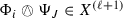
Let $J=(j_1,\dots ,j_\ell )$ be an $\ell$-tuple of integers satisfying $1\leqslant j_d\leqslant m$ for each $1\leqslant d\leqslant \ell$, where $1\le \ell \le n$. Then, . In particular, has finite $C^0$ norm (with respect to $g_t$) and . Furthermore, the harmonic projection

(3.19)

exists (and is in $\mathcal {A}_{(2)}^{(0,\ell )}(\wedge ^\ell TM_t)$) and varies smoothly in t.

Proof

By Lemma 1, one has $\Phi _{j_i}\in \widetilde{\mathcal {A}}^{0,1}(\Omega _{\overline{M}_t}(\log D_t)^\vee )$ for each $1\le i\le \ell$. By straightforward computations, one easily checks that and is $\overline{\partial }$-closed (cf. Definition 3 and [21, Remark 2]). Together with the fact that $g_t$ has Poincaré growth near $D_t$ (cf. Proposition 1), it follows readily that has finite $C^0$ norm (with respect to $g_t$), and thus it is $L^2$-integrable on $M_t$. Hence from $L^2$ Hodge decomposition as given in Lemma 2, it follows that exists and is in $\mathcal {A}_{(2)}^{0,\ell }(M_t, \wedge ^\ell TM_t)$. The smooth dependence of $\Psi _J$ on t follows from Lemma 2. $\square$

3.4 .

The use of $L^2$ condition is illustrated by the following simple lemma. Similar ideas would be used throughout our ensuing discussion to justify various integration by parts arguments.

Lemma 4

Let X be a complete Kähler manifold of complex dimension n.

• (a) Let f be an $L^2$ differentiable functions on X. Let $\gamma$ be an $L^2$ d-closed $2n-1$ form on X. Then, $\int _X df\wedge \gamma =0$.

• (b) Let $\alpha , \beta$ be $L^2$ forms on X so that $\overline{\partial }{\alpha }\wedge \beta$ is an (n, n)-form. Assume that $\beta$ is $\overline{\partial }$-closed. Then $\int _X \overline{\partial }{\alpha }\wedge \beta =0$.

Proof

(a) follows from Stokes Theorem, which follows from the trick of Gaffney [9]. More specifically, let $x_o$ be a fixed point on X. For each $r>0$, denote by $B_r$ the geodesic ball of radius r centered at $x_o$ with respect to the Kähler metric on X. For each $R>0$, define a cut-off function $\rho _R$ on X, such that $\rho _R$ takes the value 1 on $B_R$ and the value 0 on $X\setminus B_{3R}$, $0\le \rho _R(x)\le 1$ for all $x\in B_{3R}\setminus B_R$, and its covariant derivative satisfies $\Vert \nabla \rho _R(x)\Vert \le \frac{1}{R}$ for all $x\in B_{3R}\setminus B_R$. Then, from the usual Stokes Theorem, one has

$$\begin{aligned} \int _X \rho _R df\wedge \gamma =-\int _{B_{3R}} f d\rho _R\wedge \gamma . \end{aligned}$$

(3.20)

Upon applying Cauchy–Schwarz inequality to the right-hand side of (3.20) and letting $R\rightarrow \infty$, one easily concludes that $\int _X df\wedge \gamma =0$. Finally (b) follows from an easy adaptation of the above argument with the left-hand side of (3.20) replaced by the integral $\int _X\rho _R \overline{\partial }{\alpha }\wedge \beta$. $\square$

4 Computation of Curvature

4.1 .

Let $\pi :\mathcal {X}\rightarrow S$ be an effectively parametrized holomorphic family of log-canonically polarized complex manifolds over an m-dimensional complex manifold S as in Theorem 1. As in Lemma 1, we write $\pi ^{-1}(t)=M_t=\overline{M_t}\setminus D_t$ and $D_t=\sum _{i=1}^\ell D_{t,i}$ for each $t\in S$. Recall that there exists a smooth family of complete Kähler–Einstein metrics $g_t$ of constant Ricci curvature k on $M_t$ with $k<0$ and independent of $t\in S$ (cf. Proposition 1 and 2.3 and 2.4). In Sects. 4 and 5, we are going to compute the curvature tensor of the the Weil-Petersson pseudometrics on S. From now on, we follow the same notation as in [21] and refer the reader to [21] for any unexplained notation.

Let $\ell$ be an integer satisfying $1\le \ell \le n$. Recall from (3.1) the $L^2$ inner product on $M_t$ given by $(\Phi ,\Psi )=\int _{M_t} \langle \Phi ,\Psi \rangle \dfrac{\omega ^n}{n!}$ for $\Phi ,\Psi \in \mathcal {A}_{(2)}^{0,\ell }(M_t, \wedge ^\ell TM_t)$, where $\omega$ is as in (2.3), and $\langle ~,~\rangle$ denotes the pointwise inner product as in [21, equation (3.8)]. Recall also the associated $L^2$ norm given by $\Vert \Phi \Vert _{2}=\sqrt{(\Phi ,\Phi )}$. Then, as in [21, equation (3.10)], the generalized Weil-Petersson pseudo-metric on $\otimes ^\ell TS$ is defined as follows: for each $t\in S$ and $u_1,\dots ,u_\ell ,u'_1,\dots ,u'_\ell \in T_tS$, we have, in terms of (3.1),

(4.1)

Here, each $\Phi (u_i)$ is the harmonic representative of $\rho _t(u_i)$ as given in (2.4). Note that by Lemma 3 and the Cauchy–Schwarz inequality, the right hand side of (4.1) is finite. It also follows readily from Lemma 2 that the pseudometric defined in (4.1) varies smoothly in t.

To compute the curvature of the Weil–Petersson pseudometric in (4.1), we let $W\cong \Delta ^m$ be a coordinate open subset of S with coordinates $t=(t^1,\cdots , t^m)$. For each $1\le i\le m$, we recall the horizontal lifting $v_i$ and the harmonic representative $\Phi _i$ of $\rho _t(\frac{\partial }{\partial t^i})$ on $M_t$ as given in 2.4. Note that, it follows readily from (2.5) and (2.6) that $v_i$ and $\Phi _i$ vary smoothly in t. Similar to [21, Proposition 4] in the compact case, the key formula for our computation in the present non-compact case is the following

Proposition 2

Let $J=(j_1,\dots ,j_\ell )$ be an $\ell$-tuple of integers satisfying $1\leqslant j_d\leqslant m$ for each $1\leqslant d\leqslant \ell$, and let be as in (3.19). We have

Here, $\mathcal {L}_{v_i}\Psi _J$ denotes the Lie derivative of $\Psi _J$ with respect to $v_i$, and $\overline{\Phi _i}\cdot \Psi _J$ is as in [21, equation (5.6)], etc.

In this and the next section, we will give the proof of Proposition 2, dividing it into several lemmas and following the steps of proof of [21, Proposition 4]. As such, we will only give the details in those places where we need to pay attention to the non-compactness of the manifolds involved. In the process, the unexplained terms will carry the same meaning as in [21].

Remark 6

We remark that in the proofs of the lemmas leading to Proposition 2, the expressions involved will all be well-defined since all the tensors involved are $L^2$-integrable with respect to the Kähler–Einstein metric on $M_t$ for $t\in S$. In particular, as all curvature tensors involved are bounded (cf. Proposition 1), the integrals involving curvature everywhere are well-defined and finite. Recall also from Lemma 1 and Lemma 3 that all the harmonic representatives of Kodaira–Spencer classes involved are $L^2$-integrable. Thus, we typically only need to apply Hölder’s inequality to show that all expressions involved in the proof of the these lemmas are integrable. Note that from the standard use of cut-off functions as given by Gaffney in [9], all steps involving integration by parts makes sense once they are integrable according to Lemma 4.

4.2 .

For a relative tensor $\Upsilon \in \oplus _{p,q,r,s}\mathcal {A}^{q,p}(\wedge ^rTM_t\wedge \overline{\wedge ^sTM_t})$, we denote by $\Upsilon ^{(q,p)}_{(r,s)}$ the component of $\Upsilon$ in $\mathcal {A}^{q,p}(\wedge ^rTM_t\wedge \overline{\wedge ^sTM_t})$. Comparing to [21], the following lemma, which generalizes [21, Lemma 3] to our present non-compact setting, is another main technical step in this article.

Lemma 5

With notation and setting as in Proposition 2, the following statements hold.

• (a) The relative tensor $(\mathcal {L}_{\overline{v}_i}\Psi _J)_{(\ell ,0)}^{(0,\ell )}\in \mathcal {A}^{0,\ell }_{(2)}(\wedge ^\ell TM_t)$ on each $M_t$ and satisfies

  $$\begin{aligned} (\mathcal {L}_{\overline{v}_i}\Psi _J)_{(\ell ,0)}^{(0,\ell )}=\overline{\partial }\varphi \quad \text {on each }M_t \end{aligned}$$

  (4.2)

  for some relative tensor $\varphi \in \mathcal {A}^{0,\ell -1}_{(2)}(\wedge ^\ell TM_t)$. In particular, we also have $\overline{\partial }\varphi \in \mathcal {A}^{0,\ell }_{(2)}(\wedge ^\ell TM_t)$.

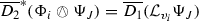
• (b) The relative tensor $\overline{D_2}^*((\mathcal {L}_{\overline{\varphi }_i}\Psi _J)^{(0,\ell )}_{(\ell ,0)})$ is $\overline{\partial }$-exact and satisfies

  $$\begin{aligned} \nabla _{\sigma }(\mathcal {L}_{\overline{\varphi }_i}\Psi _J)^{\sigma {\alpha }_1\cdots {\alpha }_{\ell -1}}_{\overline{\beta }_1\cdots \overline{\beta }_\ell } =(\overline{\partial }(\overline{\Phi _i}\cdot \Psi _J))^{{\alpha }_1\cdots {\alpha }_{\ell -1}}_{\overline{\beta }_1\cdots \overline{\beta }_\ell }\quad \text {on each }M_t, \end{aligned}$$

  (4.3)

  where the potential $\overline{\Phi _i}\cdot \Psi _J\in \mathcal {A}^{0,\ell -1}_{(2)}(\wedge ^{\ell -1}TM_t)$. Here $\overline{\Phi _i}\cdot \Psi _J$ and $\overline{D_2}^*((\mathcal {L}_{\overline{\varphi }_i}\Psi _J)^{(0,\ell )}_{(\ell ,0)})$ are as given in [21, p. 562-563].

Proof

The main difficulty is the proof of (a). We can understand the proof from two perspectives, either from the point of view of the complete metric on the non-compact manifold $M_t$, or log bundles on the compact manifolds $\overline{M}_t$.

Let us first consider a fixed fiber $M_t$. By Lemma 3, we have $\Psi _J \in \mathcal {A}^{0,\ell }_{(2)}(\wedge ^{\ell }TM_t)$ on each $M_t$. By Lemma 2,

(4.4)

for some relative tensor $K\in \mathcal {A}^{0,\ell -1}_{(2)}(\wedge ^\ell TM_t)$ which varies smoothly in t. In fact, one easily checks

(4.5)

Consider now the family of manifolds $\{M_t\}_{t\in \Delta ^m_\epsilon }$. By taking Lie derivative of the above identity, one gets

(4.6)

By [18, p. 281-282], for each $j_s$, there exists a relative tensor $K_{j_s}\in \mathcal {A}^{0,0}(TM_t)$ such that $(\mathcal {L}_{\overline{v}_i}\Phi _{j_s})^{(0,1)}_{(1,0)}=\overline{\partial }K_{j_s}$ on each $M_t$. Explicitly, by a direct computation using (2.5) and (2.6), one easily checks that $K_{j_s}$ can be given as $K_{j_s}= [\overline{v_{j_s}},v_i]^{(0,0)}_{(1,0)}$, which is easily seen to have finite $C^0$-norm (with respect to g(t)) on each $M_t$ upon following the arguments in the proof of Lemma 1. Together with (4.6) and as in [21, Lemma 3], it follows that

(4.7)

Recall from Lemma 1 that each $\Phi _{j_s}$ has finite $C^0$ norm with respect to $g_t$ on each $M_t$. It follows readily that has finite $C^0$ norm and thus it is $L^2$-integrable on each $M_t$. Thus, to complete the proof of (a), it remains to prove the following claim:

Claim: $\mathcal {L}_{\overline{v}_i}\Psi _J$ and $\mathcal {L}_{\overline{v}_i}K$ are $L^2$-integrable on each $M_t$.

Proof of Claim:

In the proof of the Claim, we will sometimes add the subscript t to relative tensors to indicate their dependence on t, so that we write $\Psi _J=\Psi _{J,t}$ and $K=K_t$ on each $M_t$, etc. Let

(4.8)

so that (4.4) becomes $\Psi _{J,t}=A_t+\overline{\partial }K_t$. By Lemma 3, $A_t$ has finite $C^0$-norm and thus it is $L^2$-integrable on each $M_t$. By Lemma 2, $\Psi _{J,t}=H_tA_t \in \mathcal {A}_{(2)}^{(0,\ell )}(\wedge ^\ell TM_t)$ and varies smoothly in t. To prove that $\mathcal {L}_{\overline{v}_i}\Psi _J$ is $L^2$-integrable on each $M_t$, we first observe that

$$\begin{aligned}&\quad \square _t \Psi _{J,t}=0\quad \text {on each }M_t \end{aligned}$$

(4.9)

$$\begin{aligned} \implies&\mathcal {L}_{\overline{v}_i}( \square _t \Psi _{J,t})=0\end{aligned}$$

(4.10)

$$\begin{aligned} \implies&\square _t (\mathcal {L}_{\overline{v}_i}\Psi _{J,t})=- ( \mathcal {L}_{\overline{v}_i}\square _t)\Psi _{J,t} \quad \text {on each }M_t . \end{aligned}$$

(4.11)

Note that $\mathcal {L}_{\overline{v}_i}\square _t$ is a second order differential operator on $M_t$. Together with (4.9), one sees from standard Calderon–Zygmund estimates (cf. e.g. [5]) that $( \mathcal {L}_{\overline{v}_i}\square _t)\Psi _{J,t}$ (and thus the right hand side of (4.11)) is $L^2$-integrable on $M_t$. Now we consider the heat equation (3.11) (with $A_t(x,\lambda )$ as given there) and $A_t$ as in (4.8). Note that from (3.19) and the proof of Lemma 2, one has $\Psi _{J,t}(x)=\displaystyle \lim _{\lambda \rightarrow \infty }A_t(x,\lambda )$ for all $x\in M_t$. Now consider the heat equation

$$\begin{aligned} \bigg \{\begin{array}{ccc} \left( \dfrac{\partial }{\partial \lambda }+\square _t\right) P_t(x,\lambda ) &{}=&{}- ( \mathcal {L}_{\overline{v}_i}\square _t)\Psi _{J,t} ,\\ P_t(x,0)&{}=&{}\mathcal {L}_{\overline{v}_i}A_t(x) \end{array} \end{aligned}$$

(4.12)

on $M_t$. We have seen that both $- ( \mathcal {L}_{\overline{v}_i}\square _t)\Psi _{J,t}$ and $\mathcal {L}_{\overline{v}_i}A_t(x)$ are $L^2$-integrable on each $M_t$. Now regularity results of parabolic equation or heat kernel estimates allow us to conclude from (4.12) that $P_t(x):=\displaystyle \lim _{\lambda \rightarrow \infty }\mathcal {L}_t P_t(x,\lambda )$ is $L^2$-integrable on $M_t$. It is easy to see from (4.11) and (4.12) that $P_t(x)= \mathcal {L}_{\overline{v}_i}\Psi _{J,t}(x)$ on $M_t$, and this finishes the proof that $\mathcal {L}_{\overline{v}_i}\Psi _{J,t}$ is $L^2$-integrable on $M_t$.

Next, we proceed similarly to prove that $\mathcal {L}_{\overline{v}_i}K$ is $L^2$-integrable on each $M_t$. Consider the heat equation (3.14) (with $B_t(x,\lambda )$ as given there and and $A_t$ as in (4.8). Let $F_t(x)=\displaystyle \lim _{\lambda \rightarrow \infty } B_t(x,\lambda )$ be as in (3.16), so that by (3.18), we have $G_tA_t=F_t-H_tF_t$ on each $M_t$. Together with (4.5), we have

$$\begin{aligned}&\quad K=-\overline{\partial }^*G_tA_t=-\overline{\partial }^*(F_t-H_tF_t)=-\overline{\partial }^*F_t\end{aligned}$$

(4.13)

$$\begin{aligned} \implies&\mathcal {L}_{\overline{v}_i}K=-\mathcal {L}_{\overline{v}_i}(\overline{\partial }^*F_t)=-(\mathcal {L}_{\overline{v}_i}\overline{\partial }^*)F_t-\overline{\partial }^*(\mathcal {L}_{\overline{v}_i}F_t) \quad \text {on each }M_t. \end{aligned}$$

(4.14)

Recall from (3.17) and (3.19) that we have

$$\begin{aligned}&\quad \square _t F_t =A_t-\Psi _{J,t}\end{aligned}$$

(4.15)

$$\begin{aligned} \implies&\square _t (\mathcal {L}_{\overline{v}_i}F_t) =\mathcal {L}_{\overline{v}_i}A_t-\mathcal {L}_{\overline{v}_i}\Psi _{J,t}-(\mathcal {L}_{\overline{v}_i}\square _t )F_t \quad \text {on each }M_t. \end{aligned}$$

(4.16)

Now consider the heat equation

$$\begin{aligned} {\left\{ \begin{array}{ll}\, \left( \dfrac{\partial }{\partial \lambda }+\square _t\right) Q_t(x,\lambda )= \mathcal {L}_{\overline{v}_i}A_t-\mathcal {L}_{\overline{v}_i}\Psi _{J,t}-(\mathcal {L}_{\overline{v}_i}\square _t )F_t ,\\ \,Q_t(x,0)=0 \end{array}\right. } \end{aligned}$$

(4.17)

We have seen that both $\mathcal {L}_{\overline{v}_i}A_t$ and $\mathcal {L}_{\overline{v}_i}\Psi _{J,t}$ are $L^2$-integrable on each $M_t$. By Lemma 2, $F_t$ is $L^2$-integrable on each $M_t$. By Lemma 3, both terms on the right-hand side of (4.15) are $L^2$-integrable on each $M_t$. Recall that $\mathcal {L}_{\overline{v}_i}\square _t$ is a second order differential operator on $M_t$. Together with (4.15), one sees from Calderon–Zygmund estimates that $( \mathcal {L}_{\overline{v}_i}\square _t)F_t$ is also $L^2$-integrable on $M_t$. Thus, all three terms on the right-hand side of (4.17) are $L^2$-integrable on each $M_t$. As before, regularity results of parabolic equation or heat kernel estimates enable us to conclude from (4.17) that $Q_t(x):=\displaystyle \lim _{\lambda \rightarrow \infty }Q_t(x,\lambda )$ is $L^2$-integrable on $M_t$. Then, one sees from (4.16) and (4.17) that $Q_t(x)= \mathcal {L}_{\overline{v}_i}F_t(x)$ on $M_t$, and this finishes the proof that $\mathcal {L}_{\overline{v}_i}F_t$ is $L^2$-integrable on $M_t$.

Next, we consider the first term $(\mathcal {L}_{\overline{v}_i}\overline{\partial }^*)F_t$ on the right-hand side of (4.16). Here, $\mathcal {L}_{\overline{v}_i}\overline{\partial }^*$ is a first-order differential operator on $M_t$. From (4.15) (and noting that both terms on its right hand side and $F_t$ are $L^2$-integrable on $M_t$), it follows that Calderon–Zygmund estimates allow us to conclude that any bounded first- and second-order derivatives of $F_t$ iare $L^2$-integrable. In particular, $(\mathcal {L}_{\overline{v}_i}\overline{\partial }^*)F_t$ is $L^2$-integrable on each $M_t$. Similarly, from (4.16) (and noting that all three terms on its right-hand side and $\mathcal {L}_{\overline{v}_i}F_t$ are $L^2$-integrable on $M_t$), it follows that Calderon–Zygmund estimates allow us to conclude that $\overline{\partial }^*(\mathcal {L}_{\overline{v}_i}F_t)$ are $L^2$-integrable on $M_t$. Since both terms on the right-hand side of (4.14) are $L^2$-integrable on $M_t$, it follows that $\mathcal {L}_{\overline{v}_i}K$ is also $L^2$-integrable on each $M_t$, and we have finished the proof of the Claim and thus also the proof of Part (a).

For Part (b), we first note that (4.3) follows from the argument of the proof of [21, Lemma 6]. By Lemma 1 and Lemma 3, $\Phi _i$ is of finite $C^0$ norm and the $\Phi _J$ is $L^2$-integrable, and this implies readily that $\overline{\Phi _i}\cdot \Psi _J$ is $L^2$-integrable on each $M_t$. Thus, we have finished the proof of Part (b). $\square$

4.3 .

The following lemma is the analogue of [21, Lemma 5].

Lemma 6

We have $\overline{\partial }^*(\overline{\Phi _i}\cdot \Psi _J)=0$.

Proof

In contrast to [21], we consider testing form $\Upsilon \in {\widetilde{\mathcal {A}}}^{0,\ell -2}(\wedge ^{\ell -1}TM_t)$ to make sure that the integration by parts in the proof of [21, Lemma 5] make sense here. Recall from Lemma 5 (b) that $\overline{\Phi _i}\cdot \Psi _J$ is $L^2$-integrable. By repeatedly using Lemma 4 (which amounts to saying that Stokes’ Theorem is valid in our situation from Gaffney’s trick) in the first two lines below, we get

(4.18)

which gives the lemma. $\square$

4.4 .

We proceed to start the proof of Proposition 2. For this purpose, we have, as in [21, equation (4.6)],

$$\begin{aligned} \partial _i\overline{\partial _i}\log \Vert \Psi _J\Vert ^2_2= & {} \partial _i\left( \frac{\partial _{\overline{i}}\Vert \Psi _J\Vert ^2_2}{\Vert \Psi _J\Vert ^2_2}\right) \nonumber \\= & {} \frac{\partial _i\partial _{\overline{i}}\Vert \Psi _J\Vert ^2_2}{\Vert \Psi _J\Vert ^2_2}-\frac{(\partial _i\Vert \Psi _J\Vert ^2_2)(\partial _{\overline{i}}\Vert \Psi _J\Vert ^2_2)}{\Vert \Psi _J\Vert ^4_2}. \end{aligned}$$

(4.19)

Following exactly the arguments in [21, pp. 559-560] with Remark 6 in mind, one has

$$\begin{aligned} \partial _i \partial _{\overline{i}} \Vert \Psi _J\Vert ^2_2&=I+II+III,\quad \text {where} \end{aligned}$$

(4.20)

$$\begin{aligned} I:&=-\int _{M_t}\langle \mathcal {L}_{\overline{v_i}}\Psi _J, \mathcal {L}_{\overline{v_i}} \Psi _J\rangle \frac{\omega ^n}{n!},\nonumber \\ II:&=\int _{M_t} \langle \mathcal {L}_{[\overline{v_i},v_i]}\Psi _J, \Psi _J\rangle \frac{\omega ^n}{n!}= (\mathcal {L}_{[\overline{v_i},v_i]}\Psi _J ,\Psi _J ),\nonumber \\ III:&=\int _{M_t}\langle \mathcal {L}_{v_i}\Psi _J, \mathcal {L}_{v_i}\Psi _J\rangle \frac{\omega ^n}{n!}=(\mathcal {L}_{v_i}\Psi _J, \mathcal {L}_{v_i}\Psi _J). \end{aligned}$$

(4.21)

The computation of the terms I, II and III will be given in Sect. 5.

5 Computation of the Terms I, II and III

5.1 .

In this section, we compute I, II and III according to the scheme of [21, Sections 5-7], except that we need to justify every step involving integration by parts, since we are considering families of non-compact manifolds. The preparation for such arguments is already presented in the previous sections. We just add the modifications at those places where necessary.

5.2 .

We begin with the computation of I. From a pointwise computation as given in [21, Section 5, pp 564-565], it follows that

$$\begin{aligned} \int _{M_t}\langle \mathcal {L}_{\overline{v_i}}\Psi _J, \mathcal {L}_{\overline{v_i}} \Psi _J\rangle \frac{\omega ^n}{n!}&= ((\mathcal {L}_{\overline{v_i}}\Psi _J)^{(0,\ell )}_{(\ell ,0)}, (\mathcal {L}_{\overline{v_i}}\Psi _J)^{(0,\ell )}_{(\ell ,0)})\nonumber \\&\quad -(\overline{\Phi _i}\searrow \Psi _J,\overline{\Phi _i}\searrow \Psi _J)- (\overline{\Phi _i}\nearrow \Psi _J,\overline{\Phi _i}\nearrow \Psi _J). \end{aligned}$$

(5.1)

Here, $\overline{\Phi _i}\searrow \Psi _J$ and $\overline{\Phi _i}\nearrow \Psi _J$ are as in [21, equation (5.10)], etc. We recall from Lemma 5 that there exists some relative tensor $K\in \mathcal {A}_{(2)}^{0,\ell -1}(\wedge ^\ell TM_t)$ such that

$$\begin{aligned} \overline{\partial }K=(\mathcal {L}_{\overline{v_i}}\Psi _J)^{(0,\ell )}_{(\ell ,0)}. \end{aligned}$$

(5.2)

Then, as in the proof of [21, Proposition 1], we have

(5.3)

In the last step, we use the proof of [21, Lemma 7] to conclude that

$$\begin{aligned} \overline{D_2}^*K=-\square (\square -k)^{-1}(\overline{\Phi _i}\cdot \Psi _J). \end{aligned}$$

(5.4)

Note again that the integrands involved in the proof of [21, Lemma 7] in our setting are all integrable according to estimates given by Lemma 5, so that the integration by parts involved can be justified (cf. Remark 6). Moreover, as $k<0$ and $\square$ is a non-negative operator, we conclude that $\square -k=\square _s-k$ for $|s|<\epsilon$ has a positive eigenvalue $\lambda _s\geqslant \eta >0$ for some $\eta$ independent of s. In particular, $(\square -k)^{-1}$ is a well-defined operator mapping a bundle-value (0, p)-form to another bundle-valued (0, p)-form. The above expression implies that

$$\begin{aligned}&((\mathcal {L}_{\overline{v_i}}\Psi _J)^{(0,\ell )}_{(\ell ,0)}, (\mathcal {L}_{\overline{v_i}}\Psi _J)^{(0,\ell )}_{(\ell ,0)})\nonumber \\&\quad = (\square (\square -k)^{-1}(\overline{\Phi _i}\cdot \Psi _J), \overline{\Phi _i}\cdot \Psi _J)\nonumber \\&\quad =k((\square -k)^{-1}(\overline{\Phi _i}\cdot \Psi _J), \overline{\Phi _i}\cdot \Psi _J)+(\overline{\Phi _i} \cdot \Psi _J,\overline{\Phi _i}\cdot \Psi _J). \end{aligned}$$

(5.5)

In summary, we have the following proposition:

Proposition 3

We have

$$\begin{aligned} I&=-k((\square -k)^{-1}(\overline{\Phi _i}\cdot \Psi _J),\overline{\Phi _i}\cdot \Psi _J) -(\overline{\Phi _i}\cdot \Psi _J,\overline{\Phi _i}\cdot \Psi _J)\nonumber \\&\quad +(\overline{\Phi _i}\searrow \Psi _J,\overline{\Phi _i}\searrow \Psi _J) +(\overline{\Phi _i}\nearrow \Psi _J,\overline{\Phi _i}\nearrow \Psi _J). \end{aligned}$$

(5.6)

Proof

The proposition is obtained by combining (4.21), (5.1) and (5.5). $\square$

5.3 .

Now, we consider the term II in (4.21). As derived from direct computations in [21, Section 6], we have

$$\begin{aligned} II=\int _{M_t}(\mathcal {L}_{[\overline{v_i},v_i]}\Psi _J)^{{\alpha }_1\cdots {\alpha }_{\ell }} _{\overline{\beta _1}\cdots \overline{\beta _\ell }}\overline{ (\Psi _J)^{\beta _1\cdots \beta _\ell }_{\overline{{\alpha }_1}\cdots \overline{{\alpha }_\ell }}} \,\frac{\omega ^n}{n!}=II_1+II_2+II_3+II_4+II_5, \end{aligned}$$

where

$$\begin{aligned} II_1:= & {} -\int _{M_t}\langle v_i,v_i\rangle ^{;\sigma }\partial _{\sigma }\big ((\Psi _J)^{{\alpha }_1\cdots {\alpha }_\ell }_{\overline{\beta _1}\cdots \overline{\beta _\ell }}\overline{ (\Psi _J)^{\beta _1\cdots \beta _\ell }_{\overline{{\alpha }_1}\cdots \overline{{\alpha }_\ell }}}\big )\frac{\omega ^n}{n!},\\ II_2:= & {} \sum _{s=1}^\ell (-1)^{s+1}\int _{M_t}\langle v_i,v_i\rangle ^{;\sigma }(\Psi _J)^{{\alpha }_1\cdots {\alpha }_{\ell }}_{\overline{\beta _1}\cdots \overline{\beta _\ell }}\overline{\partial _{\overline{{\alpha }_s}}(\Psi _J)^{\beta _1\cdots \beta _\ell }_{\overline{{\alpha }_1}\cdots \overline{{\alpha }_{s-1}}\overline{{\alpha }_{s+1}}\cdots \overline{{\alpha }_\ell }}}\frac{\omega ^n}{n!},\\ II_3:= & {} \sum _{s=1}^\ell (-1)^{s+1}\int _{M_t}\langle v_i,v_i\rangle ^{;\overline{\delta }}\partial _{\overline{\beta _s}}(\Psi _J) _{\overline{\beta _1}\cdots \overline{\beta _{s-1}}\overline{\delta }\overline{\beta _{s+1}}\cdots \overline{\beta _\ell }}\overline{ (\Psi _J)^{\beta _1\cdots \beta _\ell }_{\overline{{\alpha }_1} \cdots \overline{{\alpha }_\ell }}}\frac{\omega ^n}{n!},\\ II_4:= & {} \sum _{s=1}^\ell \int _{M_t}\partial _{{\gamma }}(\langle v_i,v_i\rangle ^{;{\alpha }_s})(\Psi _J)^{{\alpha }_1\cdots {\alpha }_{s-1}{\gamma }{\alpha }_{s+1}\cdots {\alpha }_\ell }_{\overline{\beta _1}\cdots \overline{\beta _\ell }}\overline{ (\Psi _J)^{\beta _1\cdots \beta _\ell } _{\overline{{\alpha }_1}\cdots \overline{{\alpha }_\ell }}}\frac{\omega ^n}{n!},\\ II_5:= & {} \sum _{s=1}^\ell \int _{M_t}\partial _{\overline{\beta _s}}(\langle v_i,v_i\rangle ^{;\overline{\delta }})(\Psi _J)^{{\alpha }_1\cdots {\alpha }_\ell }_{\overline{\beta _1}\cdots \overline{\beta _{s-1}}\overline{\delta }\overline{\beta _{s+1}}\cdots \overline{\beta _\ell }}\overline{ (\Psi _J)^{\beta _1\cdots \beta _\ell }_{\overline{{\alpha }_1}\cdots \overline{{\alpha }_\ell }}}\frac{\omega ^n}{n!}. \end{aligned}$$

First, we consider $II_1$. From the expression of $v_i$ in (2.5), we know that $\overline{\partial }(\langle v_i,v_i\rangle )$ is of finite $C^0$-norm on $M_t$. The expression $(\Psi _J)^{{\alpha }_1\cdots {\alpha }_{\ell }} _{\overline{\beta _1}\cdots \overline{\beta _\ell }}\overline{ (\Psi _J)^{\beta _1\cdots \beta _\ell }_{\overline{{\alpha }_1}\cdots \overline{{\alpha }_\ell }}}$ is also $L^1$-integrable from Lemma 3. Hence upon integrating by parts, one easily sees that

$$\begin{aligned} II_1=-\int _{M_t}(\square \langle v_i,v_i\rangle )\cdot \langle \Psi _J,\Psi _J\rangle \frac{\omega ^n}{n!}. \end{aligned}$$

(5.7)

Now, we consider $II_2+II_4$, which is given by

$$\begin{aligned} II_2+II_4&= \int _{M_t}(\Psi _J)^{{\alpha }_1\cdots {\alpha }_\ell } _{\overline{\beta _1}\cdots \overline{\beta _\ell }}\overline{(\overline{\partial }\Upsilon ) ^{\beta _1\cdots \beta _\ell }_{\overline{{\alpha }_1}\cdots \overline{{\alpha }_\ell }}}\frac{\omega ^n}{n!}, \quad \text {where} \end{aligned}$$

(5.8)

$$\begin{aligned} \Upsilon ^{\beta _1\cdots \beta _{\ell }}_{\overline{{\alpha }_1}\cdots \overline{{\alpha }_{\ell -1}}}&: =\overline{\langle v_i,v_i\rangle ^{;\sigma }}(\Psi _J)_{\overline{\sigma }\overline{\alpha }_1\cdots \overline{\alpha }_{\ell -1}}^{\beta _1\cdots \beta _\ell }. \end{aligned}$$

(5.9)

As mentioned earlier, $\overline{\partial }(\langle v_i,v_i\rangle )$ is of finite $C^0$-norm on $M_t$. Together with (5.9) and the fact that $\Psi _J$ is $L^2$-integrable on $M_t$, it follows readily that $\Upsilon$ (and $\Psi _J$) are $L^2$-integrable on $M_t$. Hence by integration by parts (or Lemma 4(b)), as $\overline{\partial }^*\Psi _J=0$, it follows from (5.8) that $II_2+II_4=0$. Similarly,

$$\begin{aligned} II_3+II_5&=\int _{M_t}(\overline{\partial }{\widehat{\Upsilon }})^{{\alpha }_1\cdots {\alpha }_\ell }_{\overline{\beta _1}\cdots \overline{\beta _\ell }}\overline{ (\Psi _J)^{\beta _1\cdots \beta _\ell } _{\overline{{\alpha }_1}\cdots \overline{{\alpha }_\ell }}}\frac{\omega ^n}{n!}=0,\quad \text { where}\\ {\widehat{\Upsilon }}^{{\alpha }_1\cdots {\alpha }_\ell } _{\overline{\beta _1}\cdots \overline{\beta _{\ell -1}}}&:=\langle v_i,v_i\rangle ^{;\overline{\delta }}(\Psi _J)^{{\alpha }_1\cdots {\alpha }_\ell } _{\overline{\delta }\overline{\beta _1}\cdots \overline{\beta _{\ell -1}}} . \end{aligned}$$

Hence, we have $II=II_1$. The same argument as in the last few lines of the proof of [21, Proposition 2] implies that

$$\begin{aligned} II= & {} (\mathcal {L}_{[\overline{v_i},v_i]}\Psi _J,\Psi _J)\nonumber \\= & {} -(\square \langle v_i,v_i\rangle ,\langle \Psi _J,\Psi _J\rangle )\nonumber \\= & {} -(\square (\square -k)^{-1}\langle \Phi _i,\Phi _i\rangle ,\langle \Psi _J,\Psi _J\rangle )\nonumber \\= & {} -(\langle \Phi _i,\Phi _i\rangle ,\langle \Psi _J,\Psi _J\rangle ) -k((\square -k)^{-1}\langle \Phi _i,\Phi _i\rangle ,\langle \Psi _J,\Psi _J\rangle ). \end{aligned}$$

(5.10)

In summary, we have proved the following

Proposition 4

We have

$$\begin{aligned} II=-(\langle \Phi _i,\Phi _i\rangle ,\langle \Psi _J,\Psi _J\rangle ) -k((\square -k)^{-1}\langle \Phi _i,\Phi _i\rangle ,\langle \Psi _J,\Psi _J\rangle ). \end{aligned}$$

(5.11)

5.4 .

We proceed to consider the term III in (4.21). We are going to check that the arguments of [21, Section 7], which in turn is a generalization of arguments of Siu in [18, pp. 287-295], is valid in our setting. Let $\ell$ be a fixed integer satisfying $1\leqslant \ell \leqslant n$. We denote by $X^{(\ell )}$ the space of (relative) tensors $\Xi \in \mathcal {A}(\overline{\otimes ^{\ell } T^\vee M_t}\otimes \overline{\otimes ^{\ell } T^\vee M_t})$ with components $\Xi _{\overline{{\alpha }_1}\cdots \overline{{\alpha }_\ell },\overline{\beta _1}\cdots \overline{\beta _\ell }}$ possessing the following four properties:

• (P-i) $\Xi _{\overline{{\alpha }_1}\cdots \overline{{\alpha }_\ell },\overline{\beta _1}\cdots \overline{\beta _\ell }}$ is skew-symmetric in any pair of indices ${\alpha }_i, {\alpha }_j$ for $i<j$.

• (P-ii) $\Xi _{\overline{{\alpha }_1}\cdots \overline{{\alpha }_\ell },\overline{\beta _1}\cdots \overline{\beta _\ell }}$ is symmetric in the two $\ell$-tuples of indices $(\overline{{\alpha }_1},\cdots ,\overline{{\alpha }_\ell })$ and $(\overline{\beta _1},\cdots ,\overline{\beta _\ell })$.

• (P-iii) For given indices ${\alpha }_1,\cdots ,{\alpha }_{\ell -1}$, and $\beta _1,\cdots ,\beta _{\ell +1}$, one has

  $$\begin{aligned} \sum _{\nu =1}^{\ell +1}(-1)^{\nu }\Xi _{\overline{{\alpha }_1}\cdots \overline{{\alpha }_{\ell -1}}\overline{\beta _\nu }, \overline{\beta _1}\cdots \widehat{\overline{\beta _\nu }}\cdots \overline{\beta _{\ell +1}}}=0, \end{aligned}$$

  where $\widehat{\overline{\beta _\nu }}$ means that the index $\overline{\beta _\nu }$ is omitted.

• (P-iv) $\Xi , \overline{D_i}\Xi , \overline{D_i}^*\Xi , \overline{D_i} \overline{D_i}^* \Xi , \overline{D_i}^* \overline{D_i} \Xi$ are all $L^2$-integrable for $i, j=1,2$.

Here, for $s=1,2$, we let $\overline{D_s}$ denote the operator on $X^{(\ell )}$ given by taking $\overline{\partial }$ on each fiber $M_t$ with respect to the s-th $\ell$-tuple of skew-symmetric indices, and we let $\overline{D_s}^*$ denote the adjoint operator of $\overline{D_s}$. In addition, we denote $\square _s= \overline{D_s}^*\overline{D_s}+\overline{D_s} \overline{D_s}^*$, and we denote by $H_t$ the harmonic projection operator on $X^{(\ell )}$ with respect to $\square _s$. The Green’s operator on $X^{(\ell )}$ with respect to $\square _s$ is denoted by $G_s$.

Then, by following the arguments in [21, Lemma 9], we obtain the following analogous lemma:

Lemma 7

For any $\Xi \in X^{(\ell )}$, we have

• (a) $\overline{D_1} \overline{D_2} \Xi = \overline{D_2} \overline{D_1}\Xi$,

• (b) $\overline{D_1}^* \overline{D_2} \Xi = \overline{D_2}\overline{D_1}^* \Xi$,

• (c) $\overline{D_1}^* \overline{D_2}^* \Xi = \overline{D_2}^* \overline{D_1}^*\Xi$,

• (d) $\overline{D_1} \overline{D_2}^* \Xi = \overline{D_2}^* \overline{D_1}\Xi$,

• (e) $\square _1\Xi \in X^{(\ell )}$,

• (f) $\square _1\Xi =\square _2\Xi$, and

• (g) if $\overline{D_1} \Xi =0$, then $(\square _1-k)^{-1} \overline{D_2}^* \Xi = \overline{D_2}^* G_2 \Xi$.

Note that the condition (P-iv) makes sure that all the arguments in [21], or more properly, in [18, pp. 289-292], apply in our setting.

Let $\Phi _i, \Psi _J$ (with $|J|=\ell$) be as in (2.6) and (3.19), respectively. By lowering indices of these objects as in [21, Section 7], we obtain corresponding covariant tensors, which will be denoted by the same symbols (when no confusion arises). Then, by following the arguments in [21, Lemma 10 and Lemma 11] (with the help of condition (P-iv) to make sure that they apply here), we obtain the following analogous lemma:

Lemma 8

• (a) For each $1\leqslant \ell \leqslant n$, we have $\Psi _J\in X^{(\ell )}$ and .

• (b) (i) ,

• (ii) , and

• (iii) $\overline{\partial }^*(\mathcal {L}_{v_i}\Psi _J)=0$.

We remark that (a) follows from the definition of $\Phi _i$ and the estimate in Lemma 1. Once the expressions involving $\Phi _i$ and $\Psi _J$ are shown to satisfy (a), the proof of (b) is the same as that of [21, Lemma 11], following earlier work of Siu in [18].

By following the arguments in [21, p. 573], we get

(5.12)

where, in the last step, we have used the fact that $H_2=H_1$ on $X^{(\ell +1)}$ (see [21, Remark 5(ii)]).

In conclusion, we have

Proposition 5

We have

(5.13)

Proof

By (4.21), we have

(5.14)

where the last line follows from (5.12) upon raising indices. $\square$

6 Completion of Proof of Theorem 1

6.1 .

In this section, we complete the proof of Proposition 2 as follows:

Proof of Proposition 2

By combining (4.21), Proposition 3, Proposition 4 and Proposition 5, we get

(6.1)

where, in the last line, we have used the following identity from [21, Lemma 12]:

(6.2)

We remark that the above identity follows from a pointwise computation, and thus is valid in our setting, since all the integrals involved are finite. Then, by combining (4.19), (6.1) and [21, equation (4.9)] (which also holds in our setting), one obtains Proposition 2 readily. $\square$

The following proposition, which is analogous to [21, Proposition 5], is a direct consequence of Proposition 2, and its proof is the same as in [21, Proposition 5]:

Proposition 6

We have

(6.3)

6.2 .

For our subsequent discussion, we will need the validity of [21, equation (8.7)] in our setting, which amounts to saying that the second term on the right hand side of (6.3) is positive.

Lemma 9

With notation and setting as in Proposition 6, we have

$$\begin{aligned} -k((\square -k)^{-1}\langle \Phi _i,\Phi _i\rangle , \langle \Psi _J,\Psi _J\rangle )>0. \end{aligned}$$

(6.4)

Proof

First we recall from [21, Lemma 8] that

$$\begin{aligned}&\quad (\square -k)^{-1}\langle \Phi _i,\Phi _i\rangle =v_i\cdot \overline{v_{i}} \end{aligned}$$

(6.5)

$$\begin{aligned} \implies&\langle \Phi _i,\Phi _i\rangle =(\square -k)f,\quad \text {where }f:=v_i\cdot \overline{v_{i}}. \end{aligned}$$

(6.6)

To show that (6.4) holds using the arguments in [18, pp. 297-298], it suffices to show that the real analytic function f is non-negative on $M_t$ (so that f is strictly positive at a generic point of $M_t$, since it is not a constant function as easily seen from (6.6)). In the case when $M_t$ is compact, as in [18] or [21, p. 577], the non-negativity of f was proved by applying Maximum Principle at the minimum point of f on $M_t$. In our present case, we apply the generalized Maximum Principle of [7] as stated in [3, p. 98]. First of all, we recall from Remark 4 that f is bounded below by some negative constant on $M_t$, so that $\inf f\in \mathbb {R}$. From [3, Theorem 3.75], there exists a sequence of points $\{x_j\}$ on $M_t$ such that $\displaystyle \lim _{j\rightarrow \infty }f(x_j)=\inf f$ and $\displaystyle \lim _{j\rightarrow \infty }\square f(x_j)\leqslant 0$. On the other hand,

$$\begin{aligned} \square f(x_j)=((\square -k)+k)f(x_j)=\langle \Phi _i,\Phi _i\rangle +kf(x_j)\ge k \cdot f(x_j). \end{aligned}$$

Since $k<0$, upon letting $j\rightarrow \infty$, we conclude readily that $\inf f\ge 0$, and the proof of the lemma is finished. $\square$

6.3 .

Recall from Sect. 2 that the Kähler–Einstein metric $g_t$ on each $M_t$ has Poincaré growth near $D_t$, and has bounded geometry. Together with the normalization given in (2.3), one easily checks that the volume of $M_t$ with respect to g(t), denoted by $\text {Vol}(M_t,g_t)$, satisfies

$$\begin{aligned} \text {Vol}(M_t,g_t)=\dfrac{(2\pi )^n(K_{\overline{M}_t}+D_t)^n}{k^n n!}=:A, \end{aligned}$$

(6.7)

and thus it is independent of $t\in S$. Here, $(K_{\overline{M}_t}+D_t)^n$ denotes the n-fold self-intersection number of $K_{\overline{M}_t}+D_t$. Next, we recall some definitions in [21, Section 9]. Let $N=n!$. Let $C_1:=\min \big \{1,\frac{1}{A}\big \}$ (with A as in (6.7)) and $a_1=1$. For $\ell \ge 2$, let $C_\ell =\frac{C_{\ell -1}}{3}=\frac{C_1}{3^{\ell -1}}$ and $a_\ell =\big (\dfrac{3a_{\ell -1}}{C_1}\big )^{N}$ be defined inductively. Now, for each $t\in S$ and $u\in T_tS$, we define

$$\begin{aligned} \Vert u\Vert _{WP,\ell }:=(\underbrace{u\otimes \cdots \otimes u}_{\ell -\text{ times }}, \underbrace{u\otimes \cdots \otimes u}_{\ell -\text{ times }})^{\frac{1}{2\ell }}_{WP}, \end{aligned}$$

(6.8)

where the right-hand side is as given in (4.1). Let $h:TS\rightarrow \mathbb {R}$ be the Finsler metric on S given by

$$\begin{aligned} h(u)=\Big (\sum _{\ell =1}^n a_\ell \Vert u \Vert _{WP,\ell }^{2N}\Big )^{\frac{1}{2N}} \quad \text {for }u\in T_tS \text { and }t\in S. \end{aligned}$$

(6.9)

As in [22], we call h the augmented Weil–Petersson metric on S.

Analogous to [21, Proposition 7], we have

Proposition 7

Let R be a local one-dimensional complex submanifold of S, and let $t_o\in R$ be a $\kappa$-stable point of R for some integer $1\le \kappa \le n$. Then

$$\begin{aligned} K(R,h\big |_R)(t_o)\le -\dfrac{C_\kappa }{\kappa ^{\frac{1}{N}} a_\kappa ^{1+\frac{1}{N}}}. \end{aligned}$$

(6.10)

Here, the notion of a ‘$\kappa$-stable point’ is as defined in [21, p. 581], and $K(R,h\big |_R)(t_o)$ denotes the Gaussian curvature of $(R,h\big |_R)$ at $t_o$.

Proof

From Lemma 9, one sees that [21, equation (8.7)] remains valid in our setting, and it follows readily that [21, Proposition 6] remains valid in our setting. With this in mind, one easily checks that the proof of Proposition 7 follows verbatim as that of [21, Proposition 7]. $\square$

Remark 7

Here, we furnish some definitions for the statement of Theorem 1 (cf. also [21, Section 3]). For a $C^2$ Finsler metric h on S, a point $t\in S$ and a non-zero tangent vector $u\in T_tS$, the holomorphic sectional curvature K(u) of h in the direction u is given by

$$\begin{aligned} K(u)=\sup _{R}K(R,h\big |_R)(t), \end{aligned}$$

(6.11)

where the supremum is taken over all local one-dimensional complex submanifolds R of S satisfying $t\in R$ and $T_tR=\mathbb Cu$, and $K(R,h\big |_R)(t)$ is the Gaussian curvature of $(R,h\big |_R)$ at t. We say that the holomorphic sectional curvature of the Finsler metric h on S is bounded above by a negative constant if there exists a constant $C>0$ such that $K(u)<-C$ for all $0\ne u\in TS$.

6.4 .

Now, we are going to complete the proof of Theorem 1 as follows:

Proof of Theorem 1

Theorem 1 follows readily from Proposition 7 (in place of [21, Proposition 7]) as explained in [21, p. 583, Proof of Theorem 1]. $\square$

References

Ahlfors, L.: Some remarks on Teichmüller’s space of Riemann surfaces. Ann. Math. 74, 171–191 (1961)
Ahlfors, L.: Curvature properties of Teichmüller’s space. J. Anal. Math. 9, 161–176 (1961/1962)
Aubin, T.: Some Non-linear Problems in Riemannian Geometry. Springer, Berlin (1998)
Andreotti, A., Vesentini, E.: Carleman estimates for the Laplace-Beltrami equation on complex manifolds. Inst. Hautes Études Sci. Publ. Math. 25, 81–130 (1965)
Calderón, A.P., Zygmund, A.: On the existence of certain singular integrals. Acta Math. 88, 85–139 (1952)
Cheeger, J.: On the Hodge theory of Riemannian pseudomanifolds. Geometry of the Laplace operator (Proc. Sympos. Pure Math., Univ. Hawaii, Honolulu, Hawaii, 1979), pp. 91-146, Proc. Sympos. Pure Math., XXXVI, Amer. Math. Soc., Providence, R.I. (1980)
Cheng, S.Y., Yau, S.-T.: On the existence of complete Kähler metric on noncompact complex manifolds and the regularity of Fefferman’s equation. Commun. Pure Appl. Math. 33, 507–544 (1980)
DiBenedetto, E.: Degenerate Parabolic Equations. Springer, New York (1993)
Gaffney, M.P.: A special Stokes’s theorem for complete Riemannian manifolds. Ann. Math. 60, 140–145 (1954)
Gaffney, M.P.: The heat equation method of Milgram and Rosenbloom for open Riemannian manifolds. Ann. Math. 60, 458–466 (1954)
Guenancia, H., Wu, D.: On the boundary behavior of Kähler-Einstein metrics on log canonical pairs. Math. Ann. 366(1–2), 101–120 (2016)
Kawamata, Y.: On deformations of compactifiable complex manifolds. Math. Ann. 235, 247–265 (1978)
Kobayashi, R.: Kähler-Einstein metric on an open algebraic manifolds. Osaka J. Math. 21, 399–418 (1984)
Milgram, A., Rosenbloom, P.: Harmonic forms and heat conduction, I: Closed Riemannian manifolds. Proc. Natl. Acad. Sci. U.S.A. 37, 180–184 (1951)
Mok, N., Zhong, J.-Q.: Compactifying complete Kähler-Einstein manifolds of finite topological type and bounded curvature. Ann. Math. 129, 417–470 (1989)
Royden, H.L.: Intrinsic metrics on Teichmüller space. In: Proceedings of the International Congress of Mathematicians (Vancouver, B. C., 1974), Vol. 2, pp. 217–221. Canad. Math. Congress, Montreal, QC (1975)
Schumacher, G.: Moduli of framed manifolds. Invent. Math. 134(2), 229–249 (1998)
Siu, Y.-T.: Curvature of the Weil-Petersson metric in the moduli space of compact Kähler-Einstein manifolds of negative first Chern class. Contributions to several complex variables, pp. 261–298, Aspects Math., E9, Vieweg, Braunschweig (1986)
Tian, G., Yau, S.-T.: Existence of Kähler-Einstein metrics on complete Kähler manifolds and their applications to algebraic geometry. Proc. Conf. San Diego. Adv. Ser. Math. Phys. 1, 574–629 (1987)
To, W.-K., Yeung, S.-K.: Kähler metrics of negative holomorphic bisectional curvature on Kodaira surfaces. Bull. Lond. Math. Soc. 43, 507–512 (2011)
To, W.-K., Yeung, S.-K.: Finsler metrics and Kobayashi hyperbolicity of the moduli spaces of canonically polarized manifolds. Ann. Math. 181(2), 547–586 (2015)
To, W.-K., Yeung, S.-K.: Augmented Weil-Petersson metrics on moduli spaces of polarized Ricci-flat Kähler manifolds and orbifolds. Asian J. Math. 22, 705–728 (2018)
Tsuji, H.: A characterization of ball quotients with smooth boundary. Duke Math. J. 57, 537–553 (1988)
Viehweg, E.: Quasi-projective moduli for polarized manifolds. Ergebnisse der Mathematik und ihrer Grenzgebiete. 3 Folge, Band 30. Springer, Berlin (1995)
Viehweg, E., Zuo, K.: Base spaces of non-isotrivial families of smooth minimal models. Complex Geometry (Göttingen, 2000), Springer, Berlin, pp. 279–328 (2002)
Wolpert, S.A.: Chern forms and the Riemann tensor for the moduli space of curves. Invent. Math. 85, 119–145 (1986)
Wu, D.: Kähler-Einstein metrics of negative Ricci curvature on general quasi-projective manifolds. Commun. Anal. Geom. 16(2), 395–435 (2008)
Yau, S.-T.: A general Schwarz lemma for Kähler manifolds. Am. J. Math. 100, 197–203 (1978)
Yeung, S.-K.: Compactification of complete Kähler manifolds with negative Ricci curvature. Invent. Math. 106, 13–26 (1991)
Zucker, S.: Hodge theory with degenerating coefficients: \(L^2\)-cohomology in the Poincaré metric. Ann. Math. 109, 415–476 (1979)
Author information
Authors and Affiliations
Corresponding author
Additional information
Publisher's Note
Springer Nature remains neutral with regard to jurisdictional claims in published maps and institutional affiliations.
The first author was partially supported by the Singapore Ministry of Education Academic Research Fund Tier 1 Grant R-146-000-254-114. The second author was partially supported by a grant from the National Science Foundation.
Rights and permissions
About this article
Cite this article
To, WK., Yeung, SK. Hyperbolicity of Moduli Spaces of Log-Canonically Polarized Manifolds. J Geom Anal 31, 2941–2969 (2021). https://doi.org/10.1007/s12220-020-00380-8
Received:
Published:
Issue Date:
DOI: https://doi.org/10.1007/s12220-020-00380-8