Crack Growth Modeling and Life Prediction of Pipeline Steels Exposed to Near-Neutral pH Environments: Stage II Crack Growth and Overall Life Prediction

Abstract

This investigation was initiated to provide governing equations for crack initiation, crack growth, and service life prediction of pipeline steels in near-neutral pH (NNpH) environments. This investigation develops a predictive model considering loading interactions occurring during oil and gas pipeline operation with underload-type variable pressure fluctuations. This method has predicted lifetimes comparable to the actual service lives found in the field. This is in sharp contrast with the predictions made by existing methods that are either conservative or inconsistent with the field observations. It has been demonstrated that large slash loads (R-ratio is 0.05), often seen during gas pipeline operation, are a major life-limiting factor and should be avoided where possible. Oil pipelines have shorter lifetime because of their more frequent pressure fluctuations and larger amplitude load cycles. The accuracy of prediction can be improved if pressure data with appropriate sampling intervals are used. The sampling interval error is much larger in the prediction of oil pipelines than gas pipelines because of their different compressibility but is minimized if the pressure sampling rate for the data is at or less than one minute.

1 Introduction

The safety of pipeline transportation is a matter of paramount importance because of the hazardous nature of the transported substances. Pipeline failures are associated with extensive losses both economic and environmental caused by the release of transported content, potential human injuries and casualties, huge repair and excavation costs, clean-up costs, and loss of pipeline content (gas or oil). Since the integrity of a pipeline can be threatened by various phenomena, threat mitigation and verification of fitness for service are challenges that the pipeline operators must overcome.

Near-neutral pH stress corrosion cracking (SCC) constitutes a major integrity concern to buried pipeline steels worldwide. In Reference 1 crack initiation and early-stage crack growth have been modeled. The life time spent in Stage I[1] can vary depending on the corrosion behavior of pipeline steels in near-neutral pH environments. Pipeline integrity maintenance incorporates a dual protective mechanism from the soil environments using a protective coating and cathodic protection (CP). Despite these protective measures, damage of coatings and establishment of corrosion conditions are not entirely avoidable so that the occurrence of crack initiation in a large pipeline becomes almost inevitable.

Stage I crack formation and growth[1] usually lead to dormant cracks with a depth of about 1.0 mm and since these cracks are dormant they may not form any concerns from an integrity management point of view. However, there are still less than 5 pct of cracks that are able to grow out of the dormant state.[2] It has been extensively studied that continuous growth beyond Stage I is possible if all of the following conditions are met:

• (1) Sufficient mechanical driving forces, which would make a crack propagate as governed by the principle of fracture mechanics although fracture mechanics considerations, are negligible in Stage I crack growth, as modeled in Reference 1.

• (2) The presence of residual stresses which would act together with the applied mechanical driving forces to either extend the period of dormancy if they are low or compressive, or shorten the dormancy when they are tensile and high, especially at the depth position where dormancy occurs.

• (3) The presence of sufficient levels of diffusible hydrogen which is a by-product of corrosion and cathodic protection and can synergistically interact with the mechanical driving forces to lower the threshold for Stage II crack growth and enhance Stage II crack growth rate.

The combined action of the above three factors can re-activate a dormant crack to grow at a rate that leads to premature failure of pipeline steels. Predicting crack growth rate and the remaining lifetime under a combined effect of the above conditions is the focus of this investigation.

To better appreciate the work presented in this investigation, the crack growth models currently adopted in pipeline industry are introduced. Three types of crack growth models are currently used by the pipeline industry. A brief description of the most widely applied crack growth approaches for pipeline steels is given below, although other models are also available.

1.1 Uniform Average Growth Rate

It assumes that the occurrence of SCC and SCC growth observed in the field is the 2nd stage which is characterized by more-or-less steady growth. Critical defect size is calculated using a fracture mechanics model and the time to failure is the difference between the critical and the current flaw depth divided by that crack growth rate (CGR).

1.2 Two Stage SCC and Fatigue Analysis

SCC occurs when crack depth is small and then becomes primarily fatigue driven once the SCC crack depth becomes sufficiently large. The depth at which fatigue governs occurs when the incremental CGR due to fatigue exceeds the average CGR for SCC. The net time to failure is the time for SCC to enlarge the flaw to the point where fatigue takes over, plus the time for fatigue to enlarge the flaw to failure.

1.3 Coupled SCC and Fatigue Analysis

Crack growth by SCC caused by time at constant stress is added to the growth by fatigue caused by stress cycles[3,4]

$$ {\text{d}}a/{\text{d}}N = \varphi C\Delta K^{n} + \left( {1/f} \right){{{\text{d}}a} \mathord{\left/ {\vphantom {{{\text{d}}a} {{\text{d}}t}}} \right. \kern-0pt} {{\text{d}}t}}, $$

(1)

where ϕC∆K ⁿ represents “Paris law” fatigue in an inert environment with an enhanced factor, ϕ, to consider corrosion fatigue (CF), da/dt represents the average CGR over a loading cycle, and f is the loading frequency.

The biggest discrepancy between the existing crack growth models and the actual mechanisms of crack initiation and growth arises largely from the following dilemmas:

• (1) Pipelines are operated under variable stresses. All existing models were established using data obtained either under a constant stress for SCC or constant amplitude cyclic loading for fatigue or corrosion fatigue.[5]

• (2) All existing models fail to consider various scenarios of load interactions (refer to the definition in the next section) which are essential to the nature of corrosion cracking of pipeline steels. All previous crack growth models generally yield a prediction that is significantly different from the real crack growth rate and the predicted life is very different from the actual pipeline service life.[6]

This investigation introduces crack growth predictive approaches built based on the latest understanding of SCC and corrosion fatigue crack growth mechanisms under actual pressure fluctuations found during pipeline operation. In particular, the prediction computation was made for environmentally assisted cracking of pipeline steels exposed to near-neutral pH environments for which the mechanisms of crack growth under variable amplitude pressure fluctuations have been determined.

2 Characteristics of Pipeline Pressure Fluctuations During Field Operation

To develop appropriate models for crack growth rate and service life prediction, the detailed conditions of mechanical loading during pipeline operation must be well characterized. In this investigation, a total of 18 pressure spectra (14 gas pipelines and four oil pipelines) from operation Canadian pipelines were analyzed to determine the nature of the pressure fluctuations.[7]

Figure 1 shows a representative situation of one type of pressure fluctuation that has been observed. It consists of pressure fluctuations with large cyclic amplitudes and those with relatively lower amplitudes (i.e., higher R-ratios, minimum pressure/maximum pressure, often called minor cycles or ripple loads).[8]

Fig. 1

The schematic illustration of an underload spectrum

Depending on the location of pipeline sections with respect to the compressor station (for gas pipelines or the pump station for oil pipelines), the pressure fluctuations could be further characterized into three types based on the relative pressure levels of the large loading events and the minor cycles, examples of which are shown in Figure 2 for both oil pipelines and gas pipelines.[7,8,9]

Fig. 2

Three types of pressure fluctuations[7,8,9] (with permission from ASCE). (a) Oil pipelines; (b) Gas pipelines

2.1 Type I: Underload Pressure Fluctuations

As shown in Figure 2, Type I pressure fluctuations are often found within 30 km downstream of a compressor station and these locations comprise more than 70 pct of in-service and hydro-test failures attributed to stress cracking.[10] The maximum pressure of the Type I fluctuations is often controlled to be at or close to the design limit, allowing fluctuations only to a level lower than the design limit. The spectrum consists of the so-called underload cycles which are large cycles with low R-ratios (min pressure/max pressure) and minor/ripple load cycles with very high R-ratios. Underload cycles in oil pipelines often have lower R-ratios, higher number of occurrences, and a faster rate of pressure changes (Figure 2(a)) than the underload cycles in gas pipelines (Figure 2(b)). Ripple load cycles are a main feature of gas pipelines.

2.2 Type II: Mean Load Pressure Fluctuations

Type II pressure fluctuation is typically observed further away from the compressor or pump station. In Type II, the mean pressure is lower than that in Type I, and pressure spikes with a pressure level above the mean pressure but below the design limit are frequently seen. The mean pressure is still not low enough to eliminate the underload fluctuations typically seen in Type I.

2.3 Type III: Overload Pressure Fluctuations

Type III fluctuations referred to as overload cycles typically exist at or close to a suction site where pressure spikes above the mean pressure, while the occurrence of underload cycles is minimized.

Because of the relatively high maximum pressure and large amplitude of pressure fluctuations, Type I pressure fluctuations are the harshest in terms of crack growth, and therefore are selected for crack growth modeling in this investigation. Typical characteristics of pressure fluctuations of gas and oil pipelines are compared in Table I. Oil pipelines are featured with very frequent underload cycles as compared with the gas pipelines. The rate of pressure fluctuations is slightly different in the loading portion and the unloading portion of underload cycles. However, the range of loading/unloading frequency is very different between oil pipelines and gas pipelines. Both the unloading and loading frequencies in oil pipelines vary over a wide range from 10⁻⁶ to 10⁻¹ Hz,[8] while they are very low and over a narrow range in gas pipelines. The number of minor cycles between two adjacent underload cycles is generally higher in gas pipelines than in oil pipelines.

Table I Characteristics of Type I Pressure Fluctuations in Gas and Oil Pipelines[8]

3 Mechanisms of Stage II Crack Growth

Because of the reduced rate of dissolution at the crack tip and the negligible contribution of dissolution to crack growth after dormancy, alternative crack growth mechanisms must be in operation to obtain significant crack growth. The stress factor or mechanical driving forces naturally become predominant in Stage II crack growth and crack growth would preferentially start at locations with higher tensile residual stresses and higher diffusible hydrogen content in the material surrounding the crack tip for a given pipeline section. The relative contribution to crack growth by mechanically driven processes and by dissolution during Stage II crack growth is compared and modeled in Reference 1. Although dissolution at the crack tip makes minor contribution to crack advance, it could blunt the crack tip because of the dissolution simultaneously occurring at the crack tip and on the crack wall near the crack tip, and thus it is considered to be beneficial.

Although it is often referred to as NNpH SCC, crack propagation has never been observed under a static loading condition in laboratory testing in this environment even at a high stress intensity factor, except during crack initiation where crack formation and early-stage growth are associated with the mechanisms of corrosion as discussed in Reference 1 and as other investigations have reported previously.[11,12,13,14,15,16,17,18,19,20,21] Even an active crack often ceases to grow when loading is switched to a static hold.[2] In contrast, crack growth is found to grow under cyclic loading above the critical fatigue threshold.[22,23] Figure 3 shows a typical example of a non-propagation scenario under static hold at two levels of maximum stress intensity factors.[2] In contrast, crack growth is observed when cyclic loading is resumed, although immediate crack growth did not occur in some environment when the applied mechanical driving force was low.

Fig. 3

Crack length increment as a function of test time in two different soil solutions[2] (with permission from Elsevier)

The results, like those shown in Figure 3, have revealed one of the most important prerequisites for the occurrence of stress cracking in pipeline steels exposed to near-neutral pH environments: the presence of cyclic loading. It has been further determined that the crack growth rate under constant amplitude loading can be described by the following equation[23]:

$$ {\frac{{{\text{d}}a}}{{{\text{d}}N}} = A \cdot \left( {\frac{{\Delta K^{\alpha } K_{\hbox{max} }^{\beta } }}{{f^{\gamma } }}} \right)^{n}} + {h}, $$

(2)

where A, n, α (=0.67), β (=0.33) and γ (=0.033) are all constants, α + β = 1, and h is the contribution of stress corrosion cracking considered in Reference 1. The magnitude of crack growth by dissolution in Stage II was found to be about one order of magnitude lower than the first term in Stage II crack growth. The overall power of the frequency, f, was found to be approximately 0.1 (n × γ), which is a factor representing the influence of the corrosion environment on the crack growth rate. The formulation of the combined factor makes it possible to model the crack growth with all the contributing factors included such as crack dimension, pressure fluctuations, materials, and environments. Although Eq. [2] has incorporated all possible environmental and mechanical factors affecting crack growth, it was established on the basis of crack growth data under constant amplitude fatigue loading with loading frequencies at and larger than 10⁻³ Hz.

One dilemma may arise when the γ value in Eq. [2] is further considered. Although γ is related to the influence of the corrosion environment, it is not clear how the corrosion environments may influence the value of γ, particularly considering the fact that corrosion makes a minor contribution to crack advance in Stage II. Further investigations have concluded that for a given pipeline system, the presence of near-neutral pH environments and high residual stresses on pipe surface determines whether a crack colony can be developed, while the presence of high diffusible hydrogen at special locations within some crack colonies is thought to determine whether repeated crack growth can occur.[2] Hydrogen produced by corrosion at the crack tip is secondary in terms of crack growth, as compared with the amount of hydrogen generated from the pipeline surface either resulting from general corrosion or from cathodic reaction. The latter agrees well with the fact that the rate of dissolution at the crack tip is minimal in Stage II growth as indicated previously.

Equation [2] predicts an increased crack growth rate with decreasing loading frequency. This growth rate dependence of loading frequency has been extensively proven through experimental simulations[22] and in Figure 4 as an example occurs up to a loading frequency of 10⁻³ Hz or higher. Further tests under a loading rate lower than 10⁻³ Hz demonstrate the breakdown of Eq. [2]. As shown in Figure 4, the crack growth rate is found to decrease with decreasing f when f is lower than 10⁻³ Hz.[22]

Fig. 4

The effect of loading frequency on crack growth rate under both constant amplitude loading and variable amplitude loading with underloads and minor cycles[22] (with permission from Elsevier)

The transition of crack growth behavior at f = 10⁻³ Hz has been recently found to be related to the saturation of hydrogen ahead of the crack tip at the peak stress of the loading cycle.[24] A theoretical model has been developed to understand this crack growth behavior transition based on hydrogen effects at the crack tip during the cyclic load condition.[24] It is assumed that the crack growth reaches a maximum rate when the hydrogen concentration at the crack tip reaches a certain value and the hydrogen equilibrium concentration in the plastic zone depends on the applied stresses. Therefore, the critical frequency separating the different growth behavior depends on the hydrogen diffusion into/out of the plastic zone in response to the variation of stresses. The model suggests that this critical frequency depends on loading condition, temperature, mechanical properties of the steel, and hydrogen diffusivity at the crack tip. It is estimated that the critical frequency is on the order of 10⁻³ Hz at room temperature, which is in very good agreement with the experimental results shown in Figure 4. The above theoretic analysis has further rationalized Eq. [3], which can be revised to Reference 24:

$$ \left( {\frac{{{\text{d}}a}}{{{\text{d}}N}}} \right)_{\text{tot}} = A\left( {\frac{{\Delta K^{2} K_{\hbox{max} } }}{{f^{0.1} }}} \right)^{N} ,\;f \ge f_{\text{critical}} , $$

(3)

where $A = \left[ {\frac{{4\sqrt {2.476} \left( {1 + \nu } \right)\varOmega }}{{3\pi \;k_{\text{B}} T\sqrt {2\pi } \ln \left( {\frac{1}{{c_{\text{o}} }}} \right)}}} \right]^{2n}$, and $N = 0.6n,$where k _B is the Boltzmann constant, T is the temperature, ν is the Poisson’s ratio, c ₀ is the atomic ratio of H/Fe away from crack tip, and Ω is the partial volume of hydrogen atom, and $N = 0.6n$. Equation [3] has provided a clear physical meaning to constant A, which is related to the rate of hydrogen diffusion, temperature, and hydrogen concentration in the material.

Pipelines are operated under variable amplitude pressure fluctuations. The problem of predicting fatigue crack growth becomes very complex when the applied load spectrum has variable amplitudes. This is commonly referred to as variable amplitude or spectrum loading. It produces the so-called memory effects or load-history interaction effects which are further elucidated below for their occurrences in pipeline steels.

• (1) Scenario 1 A previous cyclic loading with an R-ratio different from the current cyclic loading may condition the crack tip mechanically to either increase or decrease the crack growth rate of the current cycle and/or the future cycles, which is the so-called load-history-dependent load interactions.[25,26] The main physical models proposed to explain the load-interaction effects on fatigue crack growth include crack tip blunting,[27,28,29] cyclic plasticity-induced residual stress around the crack tip,[30] crack tip plasticity, and plasticity-induced crack closure.[31,32,33]

• (2) Scenario 2 The rate of pressure fluctuations may yield different time-dependent contributions to crack growth rate which may include the rate of corrosion, the rate of hydrogen segregation by diffusion to the crack tip,[2] and the degree of crack tip blunting caused by room-temperature creep,[2,34,35,36] and hydrogen-enhanced local plasticity (HELP).[37,38]

• (3) Scenarios (1) and (2) These scenarios can also mutually interact; for example, crack tip blunting caused by the situations described in Scenario 2 may lead to different stress states at the crack tip and therefore yield different load-history-dependent load interactions reflected in Scenario 1.[39]

The above load-interaction effects over a wide range of loading frequency are clearly demonstrated in Figure 4.[22] The top two curves are crack growth rates obtained under variable amplitude loads, while the two lower curves were under constant amplitude loads. The former is the so-called underload-minor load-type cycles, the Type I loading scheme shown in Figure 2. The underload cycles have the same amplitude and frequency as the constant amplitude loadings for the two lower curves. The minor cycle in the variable amplitude loading has a R-ratio (minimum stress/maximum stress) of 0.9, which is non-propagating if underload cycles are not present. It is clear from Figure 4 that the variable loading conditions have caused crack growth at a rate about one order of magnitude higher. It is also seen from Figure 4 that crack growth in air is insensitive to the loading frequency, while a strong frequency-dependent crack growth behavior is observed in NNpH environment, depending on the rate of loading. The importance of minor cycles in crack growth exists both in air and in NNpH ground water (e.g., C2). The enhancement in crack growth rate by the presence of minor cycles in air is even larger than that in the NNpH environment. In the former case, an increase of crack growth rate by a factor as high as 20 is observed when the underload-type variable amplitude fatigue loading was applied. It is about a factor of five in C2 solution. This indicates that the load-interaction effects are an intrinsic behavior of ductile materials and exist in all environmental conditions.

4 Computing Program for Crack Growth in Stage II

Based on the crack growth mechanisms being identified, Matlab codes have been written for the prediction of crack growth rate and service life of pipeline steels with Type I loading schemes shown in Figure 2. Figure 5 shows the flow chart of crack growth calculation, which consists of the following steps:

Fig. 5

Flow chart of crack growth calculation

• (1) Read pressure data input. The pressure data should be the raw pressure data before filtering except for artificial noises.

• (2) Assume an initial crack dimension which could be zero if Stage I modeling is also included.

• (3) Run the dissolution crack growth model and mechanical crack growth model, respectively.

• (4) Update the crack dimension for repeated crack growth calculation for the next crack-propagating pressure event.

Steps (1) to (4) continue until the updated crack depth is 0.4 t _w (t _w is the wall thickness of pipe). It should be pointed out that the possibility of failures solely induced by the failure pressure was not considered here since the emphasis of this work is the fatigue crack growth model.

The governing crack growth equations for each loading event and their combined effect on crack growth are further described in Appendix 1 for the purpose of simplicity. All the governing equations were constructed based on actual experimental results obtained in our laboratory.

5 Results of Crack Growth and Service Life Prediction

Based on the flow chart, pipeline service life can be predicted if the pressure data of the pipeline in consideration and other field data are available. Figure 6 shows the results of life prediction of a high-pressure gas pipeline with the underload-type loading spectrum. Three predicted service life curves are shown in Figure 6:

Fig. 6

Comparison of crack growth contributed by dissolution and mechanics

• (1) The life curve predicted solely based on the crack growth caused by dissolution only: In this prediction, the crack growth curve representing the average condition of growth profile was selected for the purpose of comparison, although the most severe failure-attributing conditions should be considered in integrity management.

• (2) The life curve predicted solely based on the crack growth in Stage II,[1] which yields a life time over one thousand years because of very benign mechanical driving forces during the initial stage of crack growth. It is also seen from the life curve that crack growth driven by mechanical driving forces becomes life-limiting only when crack depth reaches a depth of about 1.0 mm. This further indicates the importance of initial dissolution growth in providing a bridge to the crack growth in Stage II without which a prolonged dormant period and longer service life can be expected.

• (3) The life curve predicted by incorporating Stage I and Stage II crack growth, which yields a predicted life comparable to those found in the field. It should be noted that these predictions have been made without a consideration of the bulging factor that takes the effect of a curved pipe surface on the calculation of K at the crack tip into account, which would yield a shorter predicted life for deeper cracks. The predicted lifetime can also be shorter when cracks have larger 2c/a ratios because of increased K at the depth tip of a crack.

Figure 7 compares the lifetime curve of a gas pipeline with an oil pipeline. Both pipelines were operated under the Type I pressure fluctuation scheme. The oil pipeline has a much shorter predicted life because of frequent underload cycles with large stress amplitudes. The gas pipeline was operated with much fewer large-amplitude underload cycles but a higher number of minor load cycles that can also contribute to crack growth in the presence of underload cycles.

Fig. 7

Prediction on oil and gas underload-type spectra

Rainflow cycle counting has been widely used to analyze fatigue crack growth in the past.[40,41] The rainflow counting is a method for counting fatigue cycles from a time history. It reduces a spectrum of varying stress into a set of simple stress reversals. However, this counting method does not consider the sequence effects of different load cycles, failing to account for load interaction effects, which can be very significant for variable amplitude loadings. The results obtained from rainflow cycle counting analysis were generally very conservative and even irrational in some cases. For example, Reference 40 made a prediction of the lifetime of an oil pipeline both at the suction site and at the midpoint between the discharge and the suction sites. The results illustrated that larger crack growth rate at the suction site than the midpoint, which is not consistent with the fact that the midpoint was loaded to much higher pressure levels and had more low R-ratio fluctuations. It is believed that the discrepancies arise from the fact that the load-interaction effects could significantly enhance crack growth but are not considered in the rainflow cycle counting method.

Figure 8 shows an example of conservative lifetime estimate by the rainflow counting method, which was implemented in Matlab code strictly following the protocol established by ASME.[42] In order to guarantee the accuracy of the prediction, a small section of spectrum data were extracted and analyzed by the following two methods: (1) counting the cycles by the Matlab code self-developed based on ASME standard and (2) counting the cycles manually. It has been validated that the two methods yielded the same predictions.

Fig. 8

Comparison with rainflow counting method

As shown in Figure 8, the lifetime of the pipeline predicted by the rainflow cycle counting method yields a lifetime about 55.1 pct longer than the current method assuming end of life occurs when the crack reaches to 40 pct of wall thickness. In this comparison, the same Stage I growth curve was used. The difference in predicted life proves the significant effect of the load-interaction effects on crack growth. Furthermore, in Figure 8, the predictive life of 41 years made by this current model is more than 55 pct lower than the life predicted by the rainflow counting method. It proves the importance of load-interaction effects, and the improved precision of prediction can be achieved when the load-interaction effects are considered.

Pipelines are periodically inspected by performing hydrostatic tests. Each run of hydrostatic testing consists of two underload cycles with R = 0 and severe fatigue cycles with large stress amplitude. The effect of overload during hydrostatic hold at high pressure in terms of crack growth retardation would be reduced because of the direct underload following the overload.

The prediction of lifetimes shown in Figures 7 and 8 was made based on the crack growth rates under cathodic protection. It has been experimentally determined that crack growth rate can be significantly enhanced in the presence of cathodic protection.[43,44,45] This is attributed to the excessive amount of diffusible hydrogen generated. Figure 9 shows the lifetimes predicted by inputting different cathodic potential factors (see Appendix 1). A factor of 1.0 represents the crack growth rate measured at open circuit potential and a factor as high as 8.12 was measured for a surface crack tested under −0.9 V cathodic potential.[45] Unless it is specified, a factor of 5 was used for all the predictions made in this investigation for the effect of CP.

Fig. 9

Predicted lifetimes for the enhanced crack growth caused by cathodic protection

Figure 10 shows the effect of large slash loads on the lifetime predicted for a gas pipeline. A gas pipeline pressure spectrum free of the slash load was artificially added with a different number of slash underloads per year, ranging from 0 to 6 cycles. According to Reference 40, it is typical to observe six slash underloads (R-ratio is 0.05) per year in a gas pipeline spectrum. The pipeline with six slash underloads per year has a predicted life of 35.5 years, about 42.4 pct lower than the life of the pipeline without the slash loads.

Fig. 10

Slash load effects on life prediction of a gas spectrum

6 On the Accuracy of the Prediction

The current model is able to predict lifetimes that are comparable to the actual service life of pipeline steels with NNpHSCC developed during field operation. This level of accuracy of prediction has not been achieved by any previous models. The prediction could be made for an individual crack or for crack colonies with a range of conditions. In either case, higher accuracy can be achieved if the input data are specific and relevant. These input data include the following:

• (1) The corrosion constants for the equations governing crack growth in Stage I,

• (2) The type of materials and measured crack growth rate,

• (3) The pipeline specifics, especially the magnitude and distribution of residual stresses, and

• (4) The SCADA data fully capturing crack growth contributing events of pressure fluctuations.

In the majority of situations, it is hard and not necessary to make predictions for each crack in a colony, but rather to make a prediction for the crack with the largest dimension by inputting data representing the worst case scenario. This could be similar for pipelines at locations with similar soil and geological conditions. After all it is the fastest growing crack that determines when failure will occur.

The characteristics of pressure fluctuations responsible for crack growth can be varied and can be captured very accurately with existing technology. However, the current SCADA data are not recorded specifically for the purpose of making life prediction using the method being developed in this investigation.

The existing technology allows the pressure data to be recorded either at a fixed sampling rate or at any time when pressure changes are detected. The latter is commonly adopted for oil pipelines because of more frequent pressure fluctuations due to less compressible nature of liquids. For gas pipeline, the pressure is commonly recorded hourly.

A large sampling interval may miss some of the events of pressure fluctuations and may record a reduced magnitude of pressure fluctuations leading to a conservative estimate of service life. To determine the effect of different sampling intervals, a Matlab code was developed to analyze the data of pressure fluctuations obtained at different sampling intervals ranging from 1 second, 1, 5, 20, 40 minutes, and one hour.

Figure 11 shows the predicted lifetime of the same pipeline with the pressure data recorded at different time intervals. For an oil pipeline, as shown in Figure 11, the predicted lifetimes are not very sensitive to the sampling internals when they are less than 5 minutes but increase linearly with increasing sampling intervals beyond 5-minute interval. The difference in predicted lifetime between the shortest (1 second) and the longest (1 hour) is close to 60 pct.

Fig. 11

Effect of sampling intervals on the predicted lifetimes

Similar behavior has also been found in the prediction of lifetime for gas pipelines in Figure 11, except that the difference is much smaller, only about 10 pct between the shortest sampling rate (1 second) and the longest one (1 hour), reflecting rather sluggish pressure changes during gas pipeline operation, as evidenced in Table I.

7 Conclusions

A predictive model considering load interactions occurring during oil and gas pipeline operation with underload-type variable pressure fluctuations was developed. The current model has been built based on the latest understanding of stress cracking mechanisms established from extensive experimental results obtained from testing under realistic conditions typical of field operation. The predictions can be made using actual pressure data recorded during pipeline operation.

• (1) The current method has provided predicted lifetimes very comparable to the actual service lives found in the field. This forms a sharp contrast with the predictions made by existing methods that are either conservative or inconsistent with the field observations.

• (2) It has been demonstrated that large slash loads, often seen during gas pipeline operation, are a major life-limiting factor and should be avoided as much as possible. Oil pipelines have shorter lifetime because of their more frequent pressure fluctuations and larger cyclic amplitudes.

• (3) The accuracy of prediction can be improved if pressure data with appropriate sampling intervals are used. The error is much larger in the prediction of oil pipelines than the gas pipelines, but is minimal if the sampling rate is at or less than one minute. It should be pointed out that the life prediction in this work was made based on the most frequently recorded pressure data received from pipeline operators. The details of pressure sampling methodology can be found in Reference 46.

Appendix 1: Governing Equations Used in Life Prediction

1.1 Algorithm

• 1. The 1st step of raw data analysis is to define the stress intensity factor range threshold for minor cycles. This is set to be 0.59 ${\text{MPa}}\sqrt {\text{m}}$, below which crack is considered to be non-propagating.[22,47]

• 2. The 2nd step is to determine the underload cycles, which is defined as those cycles with a stress intensity factor range threshold larger than or equal to 3.3 ${\text{MPa}}\sqrt {\text{m}}.$[22,47]

• 3. The 3rd step is to divide a spectrum into cycle blocks, each of which is composed of one underload cycle and all the minor cycles before the next underload cycle.

• 4. Use the code to further characterize a spectrum to obtain the following parameters:

  • a. Loading and unloading frequency of each underload cycle.

  • b. K _max and ΔK of the loading cycle in an underload cycle.

  • c. K _max and ΔK of each minor cycle within a block.

  • d. The number of minor cycles within a block.

• 5. Computation of crack growth acceleration factor induced by different variables:

• (1) $f$is lower than $10^{ - 3} \;Hz$[22]:

  $$ \begin{aligned} \Delta {\text{a}}\; & { = }\;\sum\limits_{i = 1}^{k} {F^{i} (cp)} \cdot F^{i} (unload) \cdot F_{\hbox{max} }^{i} \\ & \cdot \left\{ {F_{af}^{i} (\Delta K_{ul} ,\Delta K_{mc} ,n)_{{f = 10^{ - 3} }} \cdot \left\{ {A \cdot \left[ {\frac{{K_{\hbox{max} ul}^{0.33} \cdot \Delta K_{ul}^{0.67} }}{{(10^{ - 3} )^{0.033} }}} \right]^{m} } \right\}_{i} } \right\}. \\ \end{aligned} $$

  (A.1)

• (2) $f$is larger than $10^{ - 3} \;Hz$[22]:

  $$ \begin{aligned} \Delta {\text{a}}\; & { = }\;\sum\limits_{i = 1}^{k} {F^{i} (cp)} \cdot F^{i} (unload) \cdot F_{\hbox{max} }^{i} \\ & \cdot \left\{ {F_{af}^{i} (\Delta K_{ul} ,\Delta K_{mc} ,n)_{{f = 10^{ - 3} }} \cdot \left\{ {A \cdot \left[ {\frac{{K_{\hbox{max} ul}^{0.33} \cdot \Delta K_{ul}^{0.67} }}{{(f)^{0.033} }}} \right]^{m} } \right\}_{i} } \right\}. \\ \end{aligned} $$

  (A.2)

All the variables and constants are defined in Table AI and all the functions are obtained curve-fitting the experimental results obtained.

Table AI Definition of Variables Appearing in Appendix 1

1.2 Model Parameters in Equations [A.1] and [A.2]

• (1) Combined factor model[23]:

  $$ \Delta {\text{a}}\;{ = }\;A \cdot \left[ {\frac{{K_{\hbox{max} ul}^{0.33} \cdot \Delta K_{ul}^{0.67} }}{{(f)^{0.033} }}} \right]^{m} ,\;A = 6.8 \times 10^{ - 8} ,\;m = 2.73. $$

  (A.3)

• (2) Factors induced by variable amplitude loadings[47]:

  • (a) If loading frequency f is lower than or equal to $10^{ - 3} \;Hz$

    $F(cp)$ is a factor reflecting the increased crack growth by cathodic protection as discussed in the text. It is assumed to be 5.0 for all the predictions made in the investigation unless it is specified otherwise. $F(cp)$ was experimentally determined to vary from 1 for the open circuit potential to 8.12 for surface cracks tested under −0.9 V cathodic potential.

    F(unload) is a factor reflecting the effect of asymmetrical loading waveform with the following values experimentally determined.[48]

    $$ F(unload) = \left\{ \begin{aligned} 1.4,if\;unloading\;rate\;is\;higher\;than\;loading\;rate \hfill \\ 1,if\;unloading\;rate\;is\;lower\;than\;loading\;rate \hfill \\ \end{aligned} \right.. $$

    (A.4)

    F _max is a correction factor to reflect the effect of K _max under variable amplitude fatigue loading. It was applied for tests with K _max higher or lower than 33${\text{MPa}}\sqrt {\text{m}}$. As shown in Figure A1(a)), the measured crack growth rate under variable amplitude fatigue loading is much higher than the predicted crack growth rate using Eq. [A.3],[23] which has not considered the effect of loading interactions.[47] Based on the results shown in Figure A1(b)), an acceleration factor, which is the ratio of the crack growth rate under variable amplitude fatigue loading over the crack growth predicted using Eq. [A.3], can be determined (black square symbol). From this, F _max is defined as the ratio of the acceleration factor over the acceleration factor obtained from tests under K _max = 33${\text{MPa}}\sqrt {\text{m}}$ (red circular symbol). The value of F _max obtained was curve-fitted to yield the expression below.

    $$ F_{\hbox{max} } = \left\{ \begin{aligned} 0.02667 \cdot K_{\hbox{max} ul} + 0.12,\;if\;K_{\hbox{max} ul} { < }33\;MPa\sqrt m \hfill \\ 1,\;if\;K_{\hbox{max} ul} \ge 33\;MPa\sqrt m \hfill \\ \end{aligned} \right.. $$

    (A.5)

    Fig. A1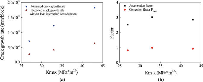

    

    Dependence of crack growth rate on K _max: (a) Measured and predicted crack growth rates[47]; (b) Crack growth acceleration caused by variable amplitude fatigue loading and the determination of F _max

    From Eq. [A.5], it is obvious that the correction factor is minimal and is needed only for tests with K _max is less than 33 ${\text{MPa}}\sqrt {\text{m}}$.

    $F_{af}^{i} \left( {\Delta K_{ul} ,\Delta K_{mc} ,n} \right)$, an acceleration factor related to the effect of ΔK _ul, ΔK _mc, and n for the ith of underload-minor cycle block, can be calculated as

    $$ F_{af} \left( {\Delta K_{ul} ,\Delta K_{mc} ,n} \right)_{{f = 10^{ - 3} }} = \frac{{F_{af} \left( {\Delta K_{ul} ,\Delta K_{mc} } \right)_{n = 300} \cdot \left( {0.05553 \cdot n^{0.6335} + 0.9258} \right)}}{{F_{af} \left( {\Delta K_{ul} = 16,\Delta K_{mc} = 3.3} \right)_{n = 300} }} $$

    (A.6)
    $$ \begin{aligned} F_{af} \left( {\Delta K_{ul} ,\Delta K_{mc} } \right)_{n = 300} & = 0.286 \cdot \left( {1 + 0.8591 \cdot \left( {0.716 \cdot \Delta K_{mc} + 0.6136} \right)^{1.41} } \right) \\ & \cdot \left( {1 + 0.1608 \cdot \left( {29.82 \cdot \Delta K_{ul}^{( - 0.8645)} } \right)^{1.693} } \right). \\ \end{aligned} $$

    (A.7)

  • (b) If loading frequency f is higher than $10^{ - 3} \;Hz$

    F(cp), F _max, and $F_{af}^{i} (\Delta K_{ul} ,\Delta K_{mc} ,n)$ are calculated in the same way as in (a).

References

J.X. Zhao, W.X. Chen, M.S. Yu, K. Chevil, R. Eadie, G. Van Boven, R. Kania, J. Been, and S. Keane: Metall. Mater. Trans. A. DOI:10.1007/s11661-016-3951-3.
W. X. Chen, R. Kania, R. Worthingham and G. Van Boven: Acta Mater., 2009, vol. 57, pp. 6200-6214.
S.B. Lambert, J.A. Beavers, B. Delanty, R. Sutherby, and A. Plumtree: Proceedings of 3rd International Pipeline Conference, Calgary, 2000, pp. 961–65.
J.A. Beavers, Near-Neutral pH SCC: Dormancy and Re-Initiation of Stress Corrosion Cracks, GRI report #: GRI-7045, August 2004.
T. S. Srivatsan and T. S. Sudarshan: J. Mater. Sci., 1988, vol. 23, pp.1521-1533.
J.F. Kiefner, and K.M. Kolovich: Predicting Times to Failure for ERW Seam Effects that Grow by Pressure-Cycle-Induced Fatigue, Final Report as the Deliverable of Subtask 2.5 on U.S. Department of Transportation, Other Transaction Agreement NO. DTPH56-11-T-000003, Final Report No. 13-021, January, 28, 2013.
Y.H. Zhang and S.J. Maddox: Int. J. Fatigue, 2009, vol. 31, pp. 138-152.
J.X. Zhao, K. Chevil, M.S. Yu, J. Been, S. Keane, G. Van Boven, R. Kania, and W.X. Chen: J. Pipeline Syst. Eng., 04016007, 2016.
J.X. Zhao, W.X. Chen, S. Keane, J. Been, and G. Van Boven: Proceedings of the 2014: 10th International Pipeline Conference IPC2014, September 29–October 3, 2014, Calgary, Alberta, Canada.
B. S. Delanty and J. O’Beirne: Oil Gas J., 1992, vol. 15, pp. 39-44.
T. Kushida, K. Nose, H. Asahi, M. Kimura, Y. Yamane, S. Endo, and H. Kawano: Proceedings of Corrosion 2001. NACE, Houston (TX), 2001. Paper No. 01223.
S. H. Wang, W. X. Chen, F. King, T. R. Jack, R. R. Fessier: Corrosion, 2002, vol. 58, pp. 526-534.
B. Y. Fang, R. L. Eadie, W. X. Chen and M. Elboujdaini: Corros. Eng. Sci. Tech., 2009, vol. 44, pp. 32-42.
B.Y. Fang, R. L. Eadie, W. X. Chen and M. Elboujdaini: Corros. Eng. Sci. Tech., 2010, vol. 45, pp. 302-312.
Z. Qin, B. Demko, J. Noel, D. Shoesmith, F. King, R. Worthingham and K. Keith: Corrosion, 2004, vol. 60, pp. 906-914.
J.A. Beavers, J.T. Johnson, R.L. Sutherby: Proceedings of 3th International Pipeline Conference, vol. 2, Calgary, Canada, October 1–5, 2000, pp. 979–88.
G. Van Boven, W.X. Chen and R. Rogge: Acta Mater., 2007, vol. 55, pp. 29-42.
B.T. Lu, and J.L. Luo: Corrosion, 2006, vol. 62, pp. 129-140.
W. Zheng, D. Bibby, J. Li, J.T. Bowker, J.A. Gianetto, R.W. Revie, and G. Williams: Proceedings of 6th International Pipeline Conference, September 25–29, 2006, p. 95.
B. Fang, E. H. Han, J. Wang, W. Ke: Corrosion, 2007, vol. 63, pp.419-432.
F. King, T. Jack, W.X. Chen, and S.H. Wang: Corrosion, 2001, NACE International, 11–16 March, Houston, Texas.
M.S. Yu, X. Xing, H. Zhang, J.X. Zhao, R. Eadie, W.X. Chen, J. Been, G. Van Boven and R. Kania: Acta Mater., 2015, vol. 96, pp.159-169.
W.X. Chen and R. L. Sutherby: Metall. Mater. Trans. A, 2007, vol. 38A, pp. 1260-1268.
X. Xing, W. X. Chen and H. Zhang: Mater. Lett., 2015, vol.152, pp. 86-89.
M. Skorupa: Fatigue Fract. Eng. Mater. Struct., 1998, vol. 21, pp.987-1006.
M. Skorupa: Fatigue Fract. Eng. Mater. Struct., 1999, vol. 22, pp. 905-926.
R.H. Christensen, Fatigue crack, fatigue damage and their directions, Metal Fatigue, McGraw-Hill, New York, 1959.
N.A. Fleck: Influence of stress state on crack growth retardation, Basic Questions on Fatigue, 1988, vol. 1, ASTM STP 924, pp. 157–83.
N.A. Fleck: Acta Metall., 1985, vol. 33, pp.1339-1354.
J. Schijve and D. Broek: Aircra. Eng. Aerosp. Tec., 1962, vol. 34, pp.314-316.
O.E. Wheeler: J. Basic Eng., 1972, vol.94, pp.181-186.
J. Willenborg, R.M. Engle, and H.A. Wood: A crack growth retardation model using an effective stress concept, Report # AFFDL-TR71-1, Air Force Flight Dynamic Laboratory, Wright-Patterson Air Force Base, USA, 1971.
S.L. Ouk and Z. W. Chen: I. J. Korean Soc. Precis. Eng., 2002, vol.3, pp.72-77.
S. H. Wang and W. X. Chen: Mater. Sci. Eng. A, 2002, vol. 325, pp.144-151.
S. H. Wang, Y. G. Zhang and W. X. Chen: J. Mater. Sci., 2001, vol. 36, pp.1931-1938.
S. H. Wang and W. X. Chen: Mater. Sci. Eng. A, 2001, vol. 301, pp.147-153.
C. D. Beachem: Met. Trans., 1972, vol. 3, pp.437-451.
P. J. Ferreira, I. M. Robertson and H. K. Birnbaum: Acta Mater., 1999, vol. 47, pp. 2991-2998.
T. M. Ahmed, S. B. Lambert, R. Sutherby and A. Plumtree: Corrosion, 1997, vol. 53, pp. 581-590.
G. Van Boven, R. Sutherby, and F. King: Proceedings of 4th International Pipeline Conference, Sep 29–Oct 3, 2002, Calgary, Canada, IPC2002-27149.
J. Schijve: Fatigue of Structures and Materials: Second Edition with CD-ROM, Springer, Dordrecht, 2009.
Standard practices for cycle counting in fatigue analysis, ASTM, E1049-85 (2011) e1.
J. Been, H. Lu, F. King, T. Jack, and R. Sutherby: Proceedings of Second International Conference on Environment-Induced Cracking of Metals (EICM-2), Banff, AB, September 20–23, Elsevier, 2004.
J. Been, R. Eadie, and R. Sutherby: Proceedings of the 2006 6th International Pipeline Conference IPC2006, September 25–29, Calgary, Alberta, Canada, IPC2006-10345.
A.T. Egbewande: Growth behavior of surface cracks in pipeline steels exposed to near-neutral pH environments. PhD thesis, University of Alberta, 2013.
J. X. Zhao, W. X. Chen, K. Chevil, J. Been, G. Van Boven, S. Keane and R. Kania: Effect of pressure sampling methods on pipeline integrity analysis. J. Pipeline Syst. Eng., Minor Revision, 2016.
M. Yu: Crack growth behavior of pipeline steels under variable pressure fluctuations in a near-neutral pH environment, PhD thesis, University of Alberta, 2015.
M. S. Yu et al. (unpublished data).
Acknowledgments
The authors would like to thank TransCanada Pipeline Limited, Spectra Energy Transmission, Natural Science and Engineering Research Council of Canada, the Pipeline Research Council International (PRCI), and US Department of Transportation for financial support.
Author information
Authors and Affiliations
Corresponding author
Additional information
Manuscript submitted January 27, 2016.