
Abstract
Wireless sensor networks (WSNs) have been the recent development in network computing and connectivity. The primary function of WSN is data extraction and transmit the collected data to remote locations. It is having very extensive application such as for monitoring, detection and identification purpose, home automation as well as industrial and healthcare applications. Despite the thriving market there are several challenges to it. For e.g. Node deployment, minimizing the power utilized, bandwidth allocation and coverage. Deployment is vital issue in WSN that affects coverage, connectivity, lifetime and many other factors of WSN. Deployment problem can also be divided into four important categories such as connectivity enhancement, coverage maximization, lifetime optimization and energy efficiency. This paper deals with the objective, strategy and constraints related to WSNs deployment as well as result oriented analysis of various deployment scheme. Also result of various deployment scheme is discussed and provided in tabular form. In conclusion, latest research issues with various possible work are debated.
1 Introduction
A sensor node, also termed as mote or sensor, is an autonomous, compact device that assimilates sensors and also contains capability to process, gather and transmit collected sensory data [1]. A sensor node collects information from sensing physical quantities such as temperature, pressure, smoke, sound etc. A wireless sensor network (WSN) refers to a group of spatially distributed sensor nodes, and one or more than one sink nodes [2]. Sink nodes are also termed as base positions. Sensors sense physical quantities such as, pressure, vibration, temperature or motion, in real time and produce sensory data [3]. A sensor acts as a data originator as well as data router. A sink node, receives and collects data from sensor nodes. In an application of event monitoring by WSN, first sensors collect information (data) from physical conditions when they sense the existence of events of interest and then sensor node conveys this collected data to the sink [4]. Sink node transmits data to the end-user by direct connections, such as satellite, internet or any other type of wireless communication. A WSN is also an environment comprised of measuring the sense data, computing, and communicating such that it provides a user the ability to observe, instrument, and respond as per the event in that particular infrastructure [5]. It comprises a large number of nodes deployed then via relay node or cluster heads, and data is passed onto the base station (sink). Here the information is being sent as a wireless link, and hence the term wireless is being used [6]. New developments in the computing hardware and software are responsible for its widespread use. In the early days, it served as the purpose in the battlefield, motivated by military applications [7]. These were used to identify, find, or detect enemy movements as well as in surveillance. However, in today’s time, the focus is on simple uses such as seismic monitoring and others directed to consumer uses. Due to the potential that WSN has its industry is overgrowing [8]. Although it can serve a lot of purposes there are major challenges to it. The lifetime of these WSN seems to be a major setback as we would require it to stay longer and in some cases a few node failures would let the entire WSN fail [9]. Also, some harsh tropical condition, enemy inhabited area would make things worse to change the batteries for these sensors [10]. Hence we would require load balancing and other deploying techniques to improve its lifetime. Another problem is coverage and one might need to cover the maximum area possible with a limited number of sensor. This would again require efficient handling of these sensors [11]. Depending upon our need we must be able to configure these sensors. Thus we would require mobile sensors. Similarly, it can be noted that mobile sinks would be a good boost in these WSNs [12]. There is sometimes the need of multi-objective sensors that not only sense the data but also performs various other tasks such as to locate a coverage hole [13], to minimize the power consumption by moving itself and likewise [14]. Also with this we need to take care of the cost as eventually we must go for a cost effective deployment techniques [15]. Some of the challenges in WSN like power consumption, localization, deployment and routing [16,17,18,19] in WSN have been represented in Fig. 1.

Challenges in WSN
Scientists are attempting to address these issues by considering different effective methodologies. This paper deals with the objective, strategy and constraints related to WSNs deployment as well as result oriented analysis of various deployment scheme. Also result of various deployment scheme is discussed and provided in tabular form.
This paper has been separated into five sections. Section 2 deals with some of the preliminary definitions, the objective, strategy and constraints related to WSNs deployment. Section 3 deals with the WSN deployment approaches which is divided into two categories: static sensor deployment and dynamic sensor deployment. Further deterministic deployment is discussed in tabular forms in reference of various coverage model. Also results of various deployment strategies are deliberated. In Sect. 4 the open research area and future work have been depicted. Lastly, this paper closes with the conclusion in Sect. 5.
2 Preliminaries
This section deals with some of the preliminary definitions, the objective, strategy and constraints related to WSNs deployment.
2.1 Preliminary Definitions
In order to understand deployment strategy in details, certain terms must be made clear. These definitions are provided here and has been illustrated in Fig. 2.
Definition I: Heterogeneous WSN These sensors are capable of doing multiple processing such as limiting power consumption, distribution of data and so on. These sensors are much more complicated to other types and pose a great deal to handle energy consumption and lifetime [20].
Definition II Homogeneous WSN They have same sensing, storage, processing, power and communication capabilities. Homogeneous WSN increases the risk of cluster head nodes being overloaded with transmissions. Hence it would require for protocol coordination and data aggregation. However, they are quite simpler to handle [21].
Definition III Relay node Relay nodes are different from other nodes as they have extra storage space to accommodate more data. Also they are accountable for accumulating sensed data and retransmitting it to sink via other relay nodes or cluster heads [22].
Definition IV Redundant node They are the similar nodes that are not used in the network for sensing. It means if removed it won’t affect the network. They are helpful in case if some nodes fail then they would take the place of the failed nodes.
Definition V Mobile node They are similar to other nodes except that they are movable and hence can change places as per our requirement. They play an important role in case of improving coverage, connectivity as well as in failure of a few nodes. Also the recovery task can be achieved when mobile node work as a router in weak or no coverage area.
Definition VI Mobile sink These are similar to mobile nodes but unlike sensing the data, they gather the sensed information. These are then used by the user. They are beneficial as it extends the network lifetime and helps in load balancing. Also energy consumption is reduced significantly [23].
Definition VII Energy hole This situation arises due to the irregular dispersal of data load on the nodes. Since the nodes closer to the sink would get heavier data traffic hence are more prone to fail. This can be corrected by deploying more redundant nodes at the sink area [24].

Preliminary definitions
2.2 The Objective of the Sensor Node Deployment
WSNs deployed to extract data from the events that happens at certain known points in a given region of interest or geographical area. WSN deployment is important to develop for real-life applications. After deployment WSN (WSN) provides too many occasions for monitoring and regulating the geographical area [25].
2.3 The Strategy of the Sensor Node Deployment
Selection of accurate position in the region of interest (RoI) is an important issue in WSNs. Sometimes requirements of system and network performance metrics are affected by the position of sensors. Vigilant deployment of sensors is very necessary to achieve the set goals [26]. If we take example of network coverage our main objective is, how to cover every target point in RoI is enclosed by the WSN. The sensor nodes placed neither too close or not too far for full utilization of sensors. A good placement of sensors will ensure a good performance for desired data extraction and communication with sink.
2.4 The Constraints of the Sensor Node Deployment
There are many constraints in deployment of WSNs, some are explained below and illustrated in Fig. 3.

Constraints of the sensor node deployment
Definition Coverage The first and most fundamental problem raises in sensors deployment, is how to cover a region of interest completely [27]. Coverage rate states to the ratio of the covered area, to the size of the RoI. Coverage rate shows great effect on the performance of WSNs. Figure 4 depicts coverage of the RoI with 120 sensors when deployed randomly in 100 × 100 m2 area with rs = 10 m.
Fig. 4 
Coverage of the RoI with 120 sensors were randomly deployed in 100 X 100 m area with rs = 10 m
Definition II:Network connectivity Connectivity is an key issue in WSN deployment [28]. WSN performance reduces exponentially without connectivity because that collected data would not reach up to the sink node. There is no benefit of coverage without connectivity in WSN deployment. Network connectivity and coverage are related to each other closely because both are affected by the position of sensors Fig. 5 represents the connectivity of 30 randomly deployed nodes.
Fig. 5 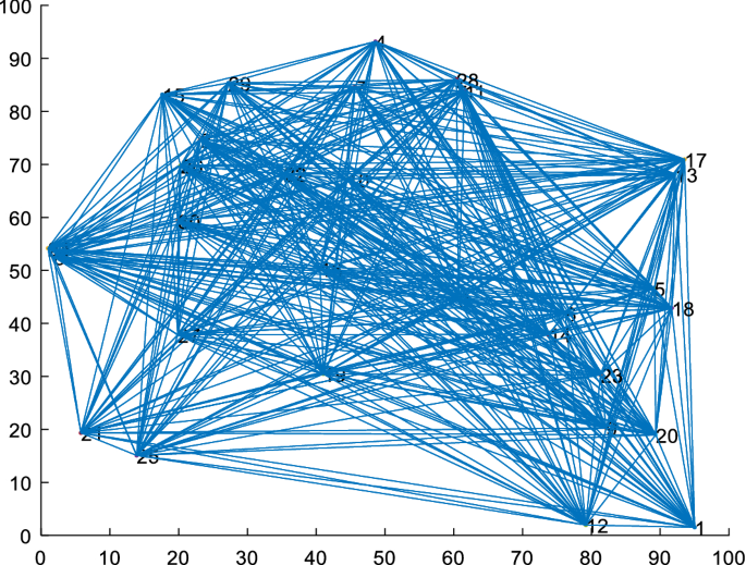
Connectivity of 30 randomly deployed sensor node inside RoI
Definition III:Network lifetime Lifetime of a network is big challenge in the deployment of WSNs because energy resources in sensors are very limited [29]. Replacing or recharging the battery of sensors after deployment is very difficult or almost impossible. Positions and number of sensors is directly proportional to lifetime of WSN. A weak lifetime of WSN is achieved when after deployment of a smaller number of sensors. But deployment of large number of sensors is not a possible solution to increase the network lifetime, because volume of traffic also increases as well as the number of sensors increases. Hence consumption of energy also increases and network lifetime of WSN decreases. Thus, deployment of larger number of sensors does not essentially solve the network lifetime problem. For the enhancement of lifetime, sensors must be placed at exact places according to many factors (signal frequency, the position of the sink).
Definition IV Energy efficiency Sensors have limited energy resources, so it is necessary to use the sensor nodes in an efficient way to enhance the lifetime of WSN [30]. There are two methods to conserve energy in sensor networks, which are connected to each other with best placement. The first method is to develop a schedule sleep plan of redundant sensors while maintaining remaining sensors in active state to maintain network connectivity and coverage. The second method for conservation of energy is regulation of the sensing range of sensors.
Definition V Signal strength Measurement of communication quality of sensor nodes called signal strength. Strength of a received wireless signal shown with parameter ‘Received signal strength indication (RSSI)’ [31]. It is defined in (1)
$$RSSI{ } = { } - 10*n*log10{ }\left( d \right) + { }P$$(1)


d = Distance from the sensor (in meter), \(n\)= Path-loss exponent (Propagation constant), \(P\)= Reception mode power (in Dbm).
Definition VI Accuracy Credibility of collected data is clearly a significant factor for WSNs deployment. Accuracy represents the efficiency in data transmission from node to destination. Data fusion increases the accuracy of the stated incident by reducing the probability of false alarms. Increasing the number of sensors RoI will increase the accuracy of the fused data.
Definition VII Deployment cost As well as number of sensors increases in WSN the deployment cost increases. In homogeneous WSNs, where all sensors have same cost, deployment cost can be decrease by achieving lowest sensor count with the satisfaction of the user’s requirements. In heterogeneous WSN, cost of deployment can be calculated by adding the costs of different type of sensors. Because various type of sensors possesses different costs, so for reducing the cost of deployment we try to find best possible combination of sensors that can satisfy requirements of application with the minimum possible cost.
3 WSN Deployment Approaches
In general, WSNs deployment divided into two categories: static sensor deployment and dynamic sensor deployment [32]. Choice of an appropriate method depends on various factors, such as the nature of the region of interest, type of sensors and the type of application. Figure 6 depicts classification of deployment techniques.

WSN deployment approaches
After deployment if sensors do not change their position, this type of deployment is known as static sensor deployment. When sensors are able to change their position this type of deployment called dynamic sensor deployment. There are two types of methods exists for static sensor deployment:
Random deployment
Deterministic deployment
3.1 Random Deployment
Random deployment is generally used in remote area, or contrary environments [33]. Deterministic deployment method is optimum if sensor nodes are deployed at predestined coordinates in RoI with the assured network connectivity. Sometimes deterministic deployment is impractical and almost impossible due to the inaccessibility or the harshness of the region of interest. In such type of situations as like natural disaster or a war, deterministic sensor deployment is very impractical and infeasible. Generally, in such type of conditions random deployment is only available option. Sometimes random deployment acts as essential part of other deployment methods. Figure 7 depicts a scenario of 324 randomly deployed nodes in 100 × 100 m2.

Random deployment N = 324 Area = 100*100 m
For example, in dynamic deployment of mobile sensors, it is assumed that initially sensor deployment takes place randomly. In random deployment, positions of sensors are shown by a mathematical function termed as probability density function (PDF). If region of interest is given as following (as in (2)):
then probability density function is given by (3):
According to the strategy of deployment, the positional coordinates of the sensors follows a specific and distinct distribution. Random deployment is categorized in two methods:
Simple random deployment
Compound random deployment
3.1.1 Simple Random Deployment
There are many methods for the implementation of simple deployment. Some methods are explained below and been depicted in Fig. 8.

Simple random deployment approach
3.1.1.1 Simple Diffusion
Simple Diffusion is a simplest way to deploy sensors. In simple diffusion we scatter sensor nodes from the air [34]. So that all extracted information must transmit up to the sink nodes, distribution must be centered on the sink node. Lightweight sensors have high air resistance so sensors can randomize their position in RoI. Such type of sensor distribution is known as simple diffusion. In simple diffusion process of deployment is characterized by a linear diffusion equation and solution of this equation is a two-dimensional normal distribution. The probability density function of locations of sensors is given in (4) and (5):
In the above equation c is the mean position at ground, c is located under the point where sensors are scattered. Here σ2 is variance and σ is standard deviation of sensor distribution. Variance is calculated by numerous factors such as weight, size and shape of sensors, or the height of scattering.
3.1.1.2 Continuous Diffusion
In continuous diffusion sensor nodes are dropped from an airplane that flies over the middle of the region of interest, in this process we expect that most sensors fall at positions which are very close to the central line [35]. Central line is represented by B. Node distribution is found uniform along the axis of flight while along the perpendicular direction of axis of flight node distribution is found Gaussian. This type of distribution of sensors is termed as continuous diffusion as shown in Fig. 9. In continuous diffusion position of sensors is decided according to the following PDF given in (6) and (7).

Continous diffusion
3.1.1.3 Discontinuous Diffusion
In discontinuous diffusion, the sensor nodes are thrown by an airplane that flies over the middle of the region of interest. The authors of [36] proposed a discontinuous diffusion of the sensor nodes defined as follows: sensors are dropped discontinuously in a one flying-over. In each drop, n sensor nodes will be thrown. Finally, for N thrown sensors,
As well as number of drops increases, discontinuous diffusion converges towards continuous diffusion.
3.1.2 Compound Random Deployment
There are many methods for the implementation of simple deployment as represented in Fig. 10. Some methods are explained below.

Compound deployment
3.1.2.1 Constant diffusion
If density of sensors remains constant in region of interest after drop of sensors, such type of random distribution of sensors is known as constant diffusion [37] as shown in Fig. 11. Position of sensors is decided according to the following PDF given in (9):

Constant diffusion
3.1.2.2 R-random
This distribution is used, if uniform scattering of sensors takes place with respect to the angular and radial directions from the sink [34]. Inside a distance R from the sink, position of sensors in polar coordinate system is decided according to PDF in (10):
3.1.2.3 Power-Law Diffusion
Power-law diffusion is random node placement algorithm in which sensor density is higher near the sink node, and a power law is followed by sensors [38]. The Probability density function of the position of sensors in polar coordinates is defined in (11):
3.1.2.4 Exponential Diffusion
In exponential diffusion, if the distribution changes according to an exponential law [39]. Exponential diffusion follows the given probability density function in (12):
Exponential diffusion takes place according to Fig. 12.

Exponential diffusion
3.1.2.5 Stensor
Stensor is a random node placement algorithm which is based on partition of RoI. In stensor algorithm, we assumed a rectangular region of interest divided into small cells. One cell can host only one sensor. Placement of sensors takes place according to the given probability density function as in (13):
3.1.2.6 Hybrid Diffusion
Hybrid diffusion is a hybridization of simple diffusion and constant diffusion [40]. Simple diffusion with large sensor count, near the sink node and constant diffusion with high network coverage and connectivity gives rise to hybrid diffusion. We select simple diffusion over the R-random because simple diffusion has a greater detection rate than R-random deployment strategy. PDF of simple diffusion is characterized by the variance \({\sigma }^{2}\) which makes it able to control the density of sensors around the sink node. Diffusion of N sensors using hybrid diffusion is same as the simple diffusion of α.N sensors and constant diffusion of β.N sensors, where α + β = 1 and 0 < α, β < 1.
3.2 Deterministic Deployment
The fundamental aim of deterministic deployment methods is to precompute the position of sensor nodes earlier to achieve the desired objectives or we try to guess performance of WSN before deployment of sensors by simulations and we develop the optimum methodology that tries to fulfil given user needs [25]. The real-world WSN deployment takes place according to obtained methodology. The fundamental concept is to confirm that the deployed WSN attains the desired goals. At present time, there is no clear methodology for deployment of a WSN that achieves the desired goals. Additionally, present work delivers algorithms of placement with no practical authentication. Generally, deterministic deployment is used for indoor applications, when sensors are costly. If operation of sensors significantly affected by their positions, such type of deployment method is used. In a comparison between deterministic and random deployment, optimum network configuration is offered by deterministic deployment. In case of deterministic deployment positions of sensors is pre-calculated to achieve the desired goals such as preferential coverage, network connectivity, and network lifetime. Figure 13 shows a scenario of 324 nodes in a RoI of 20 × 20 m2.

Deterministic deployment N = 324 Area = 20*20 m2
Coverage is considered as a most important factor in deterministic deployment. In deployment process, an algorithm in which we find maximum coverage with minimum sensor nodes is used. The taxonomy of deployment methods represents the presence of different classifications according to desired goals. Generally, sensor coverage model is divided in to three categories as shown in Fig. 14.
Binary coverage model.
Probabilistic coverage model.
Evidential coverage model.

Sensor coverage models
Based on the above coverage model, recent development in deterministic deployment is discussed below.
3.2.1 Based on Binary Coverage Model
Binary deployment methods are used if binary coverage model is used for sensor coverage model. Problem of sensor deployment in case of binary coverage model could be epitomized as the infamous Art Gallery Theorem (AGT). The art gallery problem can solve by calculating the lowest number of cameras which are positioned in a polygonal area so each point in the peripheral area is covered by cameras. Similarly, problem of sensor deployment can be solved with positioning sensors in accurate positions according to application such that whole region of interest is covered. Development and selection of optimal placement pattern is most important so that each and every point in region of interest can be covered with sensors. According to [41] regular triangular lattice can be used as placement model for blanket-cover condition of an unbounded plane. In a pattern-based/regular deployment, placement of sensors follows a set methodology such as star, ring, hexagonal etc. In a comparison between regular deployment and constant diffusion, it is found that the quality of monitoring and the covered environment in pattern-based deployment is found more effective than constant diffusion. Mathematically binary coverage models are given in (14):
where Cxy (si) represents probability of coverage of point ρ by the sensor si. d (si, ρ) is the Euclidean seperation between the node and point ρ and can be calculated by the expression in (15).
where (xi,yi) is the coordinates of the sensor si and (x, y) are the coordinates of point ρ.
In comparison among different pattern-based topologies, result comes that it is advantageous to deploy sensors using grid topology. To achieve maximum coverage with minimum sensors in the case of underwater WSN, generally triangular grid topology is used. Some authors proposed an incremental deployment process for the same. Table 1 shows some recent development in deterministic deployment techniques using Binary deployment strategies.
Sequential deployment is often infeasible because in most practical applications deployment of sensors takes place without any former information of the target. If the RoI is large or number of sensors, sequential deployment may be undesirable. Therefore, deployment method with only one step is found more beneficial in such type of situations. Problem of sensor deployment on three and two dimensional grids had been expressed as a combinatorial optimization problem and shown to be NP-complete [52]. There are two main downsides of this approach. First, the grid coverage method depends on “perfect” sensor detection concept, it means that it is expected that sensor generates binary yes/no detection result in each case. Second, due to computational complexity for large problem instances this method is found infeasible. Deployment problem of grid-based WSN has been studied widely and some methods have been intended to solve it, such as local search algorithm, simulated annealing, integer linear programming, ant colony optimization, and genetic algorithm.
It should be noted that in binary deployment strategies there is a connection between network coverage and connectivity. If we consider a convex ROI, covered by a set of sensors, it is found that communication graph containing of these sensor nodes is connected. In other words, if \({R}_{c}\) ≥ 2 \({r}_{s}\), WSN only needs to be configured to assurance coverage to satisfy both connectivity and coverage. Figure 15 shows the relationship between Communication range (\({R}_{c}\)) and Sensing range (\({r}_{s}\)) of a sensor. Hence, if the sensing range rs of a sensor is much shorter than its transmission range Rc then it is observed that connectivity is not a fundamental issue. In the case of k-coverage, same result can be generalized. In short, assurance of k-coverage also implies the assurance of k-connectivity in WSN deployment.

A sensor with communication range (\({R}_{c}\)), Sensing range (\({r}_{s}\))
3.3 Based on Probabilistic Deployment Strategies
Deployment strategies in which probabilistic sensor detection [53] takes place such type of deployment strategies refers as probabilistic deployment strategies. Figure 16 shows probability of coverage of point p for different values of ω. In probabilistic coverage model, a 2-D \(n*n\) grid is considered as RoI. Mathematically, it is given in (16):
where δ and β are constant and α is given in (17).
Table 2 shows some recent development in deployment techniques using Probabilistic deployment strategies.

Probability of coverage of point p for different values of ω
The above mentioned deployment methods can be used in the case of uniform deployment. In uniform deployment problem, recorded event has equal significance at each point of region of interest and entreated detection probabilities for complete region of interest are found same. Required detection probabilities are found different at different positions in the case of non-uniform deployment. So aforementioned placement algorithms cannot be used. Some placement algorithms for non-uniform deployment problem are mentioned below in Table 3.
3.4 Evidential Deployment Strategies
If we consider an evidential coverage model, deployment problem of WSNs solemnizes as a nonconvex and binary nonlinear optimization problem. If we take only two factors in consideration cost and uniform coverage, the authors of [67] suggested a deployment heuristic EBDA. EDBA algorithm is based on evidence and it considers grid-like node deployment. Primary objective of this algorithm, is to confirm that each target point in region of interest is covered, this projected result is the first conclusion condition. Second conclusion condition is number of available sensors. In EDBA algorithm computational complexity is equal to \(O(n.m)\), where \(n\times m\) is known as scope of the region of interest. Two other metrics, preferential coverage and connectivity have also been considered by the authors [68]. For EDBA deployment algorithm, the total number of different sub problems is an exponential in the input size. This concept gives rise to an exponential-time algorithm. A substitute E2BDA can be utilized to develop a sub optimal solution. E2BDA algorithm is considered as a polynomial-time algorithm.
E2BDA algorithm uses a restricted region which is based on the sliding window method and do not check all grid points to calculate coverage. If E2BDA having large number of sensor nodes then the computational complexity is found equal to the \(O\left(k{w}^{2}mn\right)\), Where:
\(k\): Number of best deployments at each repetition. \(w\): Window size, equal to sensing range of sensor. \(m\times n\): Size of the RoI.
Experimental results reported E2BDA outperforms these deployment strategies.
4 Open Research Issue
Since WSN is a newly developed concept, there is no universal theory applied for it. We need to choose from the techniques as per our requirement. In recent times, WSNs have garnered much attention. Although it is under constant progress, there are many grey areas left in its development.
Coverage hole detection improvement is always on everyone’s radar while studying the deployment of WSNs. The recovery mechanism for coverage hole yet seems to be a common problem in any method of deployment. The problem remains still open to detect such holes as well as repair it. Another challenge that poses to WSNs is improving node detection and connectivity recovery algorithms. In this paper, this problem is addressed, and to an extent, we can improve the node failure. However, in a limited number of nodes, re-connectivity cannot be guaranteed.
Another critical issue is improving the Energy Efficiency. As sensors run on batteries, it is evident that they would someday die. They are hence preserving energy such that it could have a long run. Efficient deployment scheme needs to be developed for sleep mode for the sensors without affecting the Quality of Service (QoS) parameters.
In cases where multiple sinks are in play, there is some adherent possibility of data aggregation. As a result, it would raise two common problems. Firstly, a wrong route to base station and secondly, a wrong route to the node. In either case, it would lead to the disruption of network communication. These must be taken care of for improving the WSNs.
5 Conclusion
In this paper, we have discussed most of the prominent deployment techniques in WSNs and identified its significant drawback as well as its advantages. Not only this, we have also discussed the challenges or precautions that arise while installation and deploying WSNs. Also, a table is drawn on comparing each of the deployment techniques in each section. A comprehensive table is drawn in the last section to give the overview and comparison of each technique discussed. We can efficiently use the schemes as per our region of operation, whether it is a 3D or 2D deployment. All other factors that are prominent while deploying WSNs have been discussed, such as cost, energy distribution, range, and availability of nodes. With the schemes discussed here, one can selectively determine the deployment technique with ease.
References
Khan, I., Belqasmi, F., Glitho, R., Crespi, N., Morrow, M., & Polakos, P. (2016). Wireless sensor network virtualization: A survey. IEEE Communications Surveys and Tutorials. https://doi.org/10.1109/COMST.2015.2412971.
Farsi, M., Elhosseini, M. A., Badawy, M., Ali, H. A., & Eldin, H. Z. (2019). Deployment techniques in wireless sensor networks, coverage and connectivity: A survey. IEEE Access,7, 28940–28954.
Toral-Cruz, H., Hidoussi, F., Boubiche, D. E., Barbosa, R., Voznak, M., & Lakhtaria, K. I. (2015). A survey on wireless sensor networks. Next Generation Wireless Network Security and Privacy. https://doi.org/10.4018/978-1-4666-8687-8.ch006.
Pantazis, N. A., Nikolidakis, S. A., & Vergados, D. D. (2013). Energy-efficient routing protocols in wireless sensor networks: A survey. IEEE Communications Surveys and Tutorials. https://doi.org/10.1109/SURV.2012.062612.00084.
Zhu, C., Zheng, C., Shu, L., & Han, G. (2012). A survey on coverage and connectivity issues in wireless sensor networks. Journal of Network and Computer Applications. https://doi.org/10.1016/j.jnca.2011.11.016.
Rawat, P., Singh, K. D., Chaouchi, H., & Bonnin, J. M. (2014). Wireless sensor networks: A survey on recent developments and potential synergies. Journal of Supercomputing. https://doi.org/10.1007/s11227-013-1021-9.
Borges, L. M., Velez, F. J., & Lebres, A. S. (2014). Survey on the characterization and classification of wireless sensor network applications. IEEE Communications Surveys and Tutorials. https://doi.org/10.1109/COMST.2014.2320073.
Rashid, B., & Rehmani, M. H. (2016). Applications of wireless sensor networks for urban areas: A survey. Journal of Network and Computer Applications. https://doi.org/10.1016/j.jnca.2015.09.008.
Yun, Y., & Xia, Y. (2010). Maximizing the lifetime of wireless sensor networks with mobile sink in delay-tolerant applications. IEEE Transactions on Mobile Computing. https://doi.org/10.1109/TMC.2010.76.
Curry, R. M., & Smith, J. C. (2016). A survey of optimization algorithms for wireless sensor network lifetime maximization. Computers and Industrial Engineering. https://doi.org/10.1016/j.cie.2016.08.028.
Fan, G., & Jin, S. (2010). Coverage problem in wireless sensor network: A survey. Journal of Networks. https://doi.org/10.4304/jnw.5.9.1033-1040.
Ramasamy, V. (2017). Mobile wireless sensor networks: An overview. Wireless Sensor Networks—Insights and Innovations. https://doi.org/10.5772/intechopen.70592.
Priyadarshi, R., & Gupta, B. (2019). Coverage area enhancement in wireless sensor network. Microsystem Technologies. https://doi.org/10.1007/s00542-019-04674-y.
Babaie, S., & Pirahesh, S. S. (2012). Hole detection for increasing coverage in wireless sensor network using triangular structure. CoRR. arXiv:1203.3772.
Priyadarshi, R., Gupta, B., & Anurag, A. (2020). Deployment techniques in wireless sensor networks: A survey, classification, challenges, and future research issues. The Journal of Supercomputing. https://doi.org/10.1007/s11227-020-03166-5.
Priyadarshi, R., Soni, S. K., & Nath, V. (2018). Energy efficient cluster head formation in wireless sensor network. Microsystem Technologies. https://doi.org/10.1007/s00542-018-3873-7.
Priyadarshi, R., Rawat, P., & Nath, V. (2019). Energy dependent cluster formation in heterogeneous wireless sensor network. Microsystem Technologies. https://doi.org/10.1007/s00542-018-4116-7.
Priyadarshi, R., Soni, S. K., & Sharma, P. (2019). An enhanced GEAR protocol for wireless sensor networks. Lecture Notes in Electrical Engineering. https://doi.org/10.1007/978-981-13-0776-8_27.
Priyadarshi, R., Singh, L., Randheer, & Singh, A. (2018). A Novel HEED Protocol for Wireless Sensor Networks. In 2018 5th international conference on signal processing and integrated networks, SPIN 2018. https://doi.org/10.1109/SPIN.2018.8474286
Srivastava, S., Singh, M., & Gupta, S. (2018). Wireless sensor network: A survey. In 2018 international conference on automation and computational engineering, ICACE 2018. https://doi.org/10.1109/ICACE.2018.8687059
Yick, J., Mukherjee, B., & Ghosal, D. (2008). Wireless sensor network survey. Computer Networks. https://doi.org/10.1016/j.comnet.2008.04.002.
Xu, K., Hassanein, H., Takahara, G., & Wang, Q. (2010). Relay node deployment strategies in heterogeneous wireless sensor networks. IEEE Transactions on Mobile Computing. https://doi.org/10.1109/TMC.2009.105.
Liang, W., Luo, J., & Xu, X. (2010). Prolonging network lifetime via a controlled mobile sink in wireless sensor networks. GLOBECOM—IEEE Global Telecommunications Conference. https://doi.org/10.1109/GLOCOM.2010.5683095.
Ren, J., Zhang, Y., Zhang, K., Liu, A., Chen, J., & Shen, X. S. (2016). Lifetime and energy hole evolution analysis in data-gathering wireless sensor networks. IEEE Transactions on Industrial Informatics. https://doi.org/10.1109/TII.2015.2411231.
Aznoli, F., & Navimipour, N. J. (2017). Deployment strategies in the wireless sensor networks: Systematic literature review, classification, and current trends. Wireless Personal Communications. https://doi.org/10.1007/s11277-016-3800-0.
Barrenetxea, G., Ingelrest, F., Schaefer, G., & Vetterli, M. (2008). The hitchhiker’s guide to successful wireless sensor network deployments. In SenSys’08–Proceedings of the 6th ACM conference on embedded networked sensor systems. https://doi.org/10.1145/1460412.1460418
Aziz, N., Aziz, K., & Ismail, W. (2009). Coverage strategies for wireless sensor networks. World academy of science, engineering and technology, open science index 26. International Journal of Electronics and Communication Engineering, 3(2), 171–176.
Boukerche, A., & Sun, P. (2018). Connectivity and coverage based protocols for wireless sensor networks. Ad Hoc Networks. https://doi.org/10.1016/j.adhoc.2018.07.003.
Wang, D., Xie, B., & Agrawal, D. P. (2008). Coverage and lifetime optimization of wireless sensor networks with Gaussian distribution. IEEE Transactions on Mobile Computing. https://doi.org/10.1109/TMC.2008.60.
Shaikh, F. K., & Zeadally, S. (2016). Energy harvesting in wireless sensor networks: A comprehensive review. Renewable and Sustainable Energy Reviews. https://doi.org/10.1016/j.rser.2015.11.010.
Xu, J., Liu, W., Lang, F., Zhang, Y., & Wang, C. (2010). distance measurement model based on RSSI in WSN. Wireless Sensor Network. https://doi.org/10.4236/wsn.2010.28072.
Patzer, A., & Patzer, A. (2002). Deployment techniques. JSP Examples and Best Practices. https://doi.org/10.1007/978-1-4302-0831-0_10.
Beutel, J., Römer, K., Ringwald, M., & Woehrle, M. (2010). Deployment techniques for sensor. Networks.. https://doi.org/10.1007/978-3-642-01341-6_9.
Ishizuka, M., & Aida, M. (2004). Performance study of node placement in sensor networks. Proceedings - International Conference on Distributed Computing Systems. https://doi.org/10.1109/icdcsw.2004.1284093.
Onur, E., Ersoy, C., Deliç, H., & Akarun, L. (2007). Surveillance wireless sensor networks: Deployment quality analysis. Network, IEEE,21, 48–53. https://doi.org/10.1109/MNET.2007.4395110.
Senouci, M. R., Mellouk, A., & Aissani, A. (2012). An analysis of intrinsic properties of stochastic node placement in sensor networks. GLOBECOM–IEEE Global Telecommunications Conference. https://doi.org/10.1109/GLOCOM.2012.6503161.
Yoo, Y.,& Agrawal, D. (2008) Mobile sensor relocation to prolong the lifetime of wireless sensor networks. In VTC spring 2008-IEEE vehicular technology conference 10.1109/VETECS.2008.52.
Ishizuka, M., & Aida, M. (2004). The reliability performance of wireless sensor networks configured by power-law and other forms of stochastic node placement. IEICE Transactions on Communications.,87, 2511–2520.
Zhang, H., & Hou, J. (2004). On deriving the upper bound of α-lifetime for large sensor networks. Proceedings of the International Symposium on Mobile Ad Hoc Networking and Computing (MobiHoc). https://doi.org/10.1145/989459.989475.
Senouci, M. R., Mellouk, A., & Aissani, A. (2014). Random deployment of wireless sensor networks: A survey and approach. International Journal of Ad Hoc and Ubiquitous Computing. https://doi.org/10.1504/IJAHUC.2014.059905.
Kershner, R. (1939). The number of circles covering a set. American Journal of Mathematics. https://doi.org/10.2307/2371320.
Wang, Y. C., Hu, C. C., & Tseng, Y. C. (2005). Efficient deployment algorithms for ensuring coverage and connectivity of wireless sensor networks. Proceedings–First International Conference on Wireless Internet, WICON. https://doi.org/10.1109/wicon.2005.13.
Carter, B., & Ragade, R. (2008). An extensible model for the deployment of non-isotropic sensors. In 2008 IEEE sensors applications symposium, SAS-2008–Proceedings.
Halder, S., & Das Bit, S. (2015). Design of an Archimedes’ spiral based node deployment scheme targeting enhancement of network lifetime in wireless sensor networks. Journal of Network and Computer Applications. https://doi.org/10.1016/j.jnca.2014.09.014.
Sahin, D., & Ammari, H. M. (2014). The art of wireless sensor networks. The Art of Wireless Sensor Networks. https://doi.org/10.1007/978-3-642-40009-4.
Fan, T., Teng, G., & Huo, L. (2014). A pre-determined nodes deployment strategy of two-tiered wireless sensor networks based on minimizing cost. International Journal of Wireless Information Networks. https://doi.org/10.1007/s10776-014-0240-1.
Yun, Z., Bai, X., Xuan, D., Lai, T. H., & Jia, W. (2010). Optimal deployment patterns for full coverage and κ-Connectivity (κ≤6) wireless sensor networks. IEEE/ACM Transactions on Networking. https://doi.org/10.1109/TNET.2010.2040191.
Iqbal, M. M., Gondal, I., & Dooley, L. (2004). Dynamic symmetrical topology models for pervasive sensor networks. In Proceedings of INMIC 2004–8th international multitopic conference. https://doi.org/10.1109/INMIC.2004.1492925
Filipe, L., Vieira, M., Augusto, M., Vieira, M., Ruiz, L. B., Alfredo, A., et al. (2004). Efficient incremental sensor network deployment algorithm. In Brazilian symposium on computer networks.
Pompili, D., Melodia, T., & Akyildiz, I. F. (2006). Deployment analysis in underwater acoustic wireless sensor networks. In WUWNet 2006 - proceedings of the first ACM international workshop on underwater networks. https://doi.org/10.1145/1161039.1161050
Coello Coello, C. A. (2002). Theoretical and numerical constraint-handling techniques used with evolutionary algorithms: A survey of the state of the art. Computer Methods in Applied Mechanics and Engineering. https://doi.org/10.1016/S0045-7825(01)00323-1.
Ke, W. C., Liu, B. H., & Tsai, M. J. (2011). The critical-square-grid coverage problem in wireless sensor networks is NP-Complete. Computer Networks. https://doi.org/10.1016/j.comnet.2011.03.004.
Hossain, A., Biswas, P. K., & Chakrabarti, S. (2008). Sensing models and its impact on network coverage in wireless sensor network. In IEEE region 10 colloquium and 3rd international conference on industrial and information systems, ICIIS 2008. https://doi.org/10.1109/ICIINFS.2008.4798455
Dhillon, S. S., Chakrabarty, K., & Iyengar, S. S. (2002). Sensor placement for grid coverage under imprecise detections. In Proceedings of the 5th international conference on information fusion, FUSION 2002. https://doi.org/10.1109/ICIF.2002.1021005
Dhillon, S. S., & Chakrabarty, K. (2003). Sensor placement for effective coverage and surveillance in distributed sensor networks. IEEE Wireless Communications and Networking Conference, WCNC.. https://doi.org/10.1109/WCNC.2003.1200627.
Huang, S.-C., Chang, H.-Y., & Wu, K.-L. (2013). A jigsaw-based sensor placement algorithm for wireless sensor networks. International Journal of Distributed Sensor Networks,2013, 1–11. https://doi.org/10.1155/2013/186720.
Wu, C. H., Lee, K. C., & Chung, Y. C. (2007). A delaunay triangulation based method for wireless sensor network deployment. Computer Communications. https://doi.org/10.1016/j.comcom.2007.05.017.
Aitsaadi, N., Achir, N., Boussetta, K., & Pujolle, G. (2007). Differentiated underwater sensor network deployment. In OCEANS 2007 - Europe. https://doi.org/10.1109/oceanse.2007.4302456.
Aitsaadi, N., Achir, N., Boussetta, K., & Pujolle, G. (2009). A Tabu search WSN deployment method for monitoring geographically irregular distributed events. Sensors. https://doi.org/10.3390/s90301625.
Senouci, M., Bouguettouche, D., Souilah, F., & Mellouk, A. (2014). Efficient heuristic for the deterministic deployment of wireless sensor networks. In The international conference META.
Senouci, M., Souilah, F., Bouguettouche, D., & Mellouk, A. (2014). Simulated annealing for solving the wireless sensor networks deployment problem. In META.
Mini, S., Udgata, S. K., & Sabat, S. L. (2013). Artificial bee colony algorithm for probabilistic target Q-coverage in wireless sensor networks. Lecture Notes in Computer Science (including subseries Lecture Notes in Artificial Intelligence and Lecture Notes in Bioinformatics). https://doi.org/10.1007/978-3-319-03753-0_40.
Senouci, M. R., Bouguettouche, D., Souilah, F., & Mellouk, A. (2016). Static wireless sensor networks deployment using an improved binary PSO. International Journal of Communication Systems. https://doi.org/10.1002/dac.3040.
Zhang, J., Yan, T., & Son, S. H. (2006). Deployment strategies for differentiated detection in wireless sensor networks. In 2006 3rd annual IEEE communications society on sensor and adhoc communications and networks, secondary, 2006. https://doi.org/10.1109/SAHCN.2006.288436.
Ababnah, A., & Natarajan, B. (2011). Optimal control-based strategy for sensor deployment. IEEE Transactions on Systems, Man, and Cybernetics Part A: Systems and Humans.. https://doi.org/10.1109/TSMCA.2010.2049992.
Ababnah, A., & Natarajan, B. (2009). Sensor deployment as an optimal control problem. Proceedings–International Conference on Computer Communications and Networks, ICCCN.. https://doi.org/10.1109/ICCCN.2009.5235252.
Senouci, M. R., Mellouk, A., Oukhellou, L., & Aissani, A. (2011). Uncertainty-aware sensor network deployment. GLOBECOM–IEEE Global Telecommunications Conference. https://doi.org/10.1109/GLOCOM.2011.6134363.
Reda, S. M., Abdelhamid, M., Latifa, O., & Amar, A. (2012). Efficient uncertainty-aware deployment algorithms for wireless sensor networks. IEEE Wireless Communications and Networking Conference, WCNC.. https://doi.org/10.1109/WCNC.2012.6214151.
Author information
Authors and Affiliations
Corresponding author
Additional information
Publisher's Note
Springer Nature remains neutral with regard to jurisdictional claims in published maps and institutional affiliations.
Rights and permissions
About this article

Cite this article
Priyadarshi, R., Gupta, B. & Anurag, A. Wireless Sensor Networks Deployment: A Result Oriented Analysis. Wireless Pers Commun 113, 843–866 (2020). https://doi.org/10.1007/s11277-020-07255-9
Published:
Issue Date:
DOI: https://doi.org/10.1007/s11277-020-07255-9