A novel approach for designing delay efficient path for mobile sink in wireless sensor networks

Abstract

In the recent years, the use of mobile sink has drawn enormous attention for data collection in wireless sensor networks (WSNs). Mobile sink is well known for solving hotspot or sinkhole problem. However, the design of an efficient path for mobile sink has tremendous impact on network lifetime and coverage in data collection process of WSNs. This is particularly an important issue for many critical applications of WSNs where data collection requires to be carried out in delay bound manner. In this paper, we propose a novel scheme for delay efficient trajectory design of a mobile sink in a cluster based WSN so that it can be used for critical applications without compromising the complete coverage of the target area. Given a set of gateways (cluster heads), our scheme determines a set of rendezvous points for designing path of the mobile sink for critical applications. The scheme is based on the Voronoi diagram. We also propose an efficient method for recovery of the orphan sensor nodes generated due to the failure of one or more cluster heads during data collection. We perform extensive simulations over the proposed algorithm and compare its results with existing algorithms to demonstrate the efficiency of the proposed algorithm in terms of network lifetime, path length, average waiting time, fault tolerance and adaptability etc. For the fault tolerance, we simulate the schemes using Weibull distribution and analyze their performances.

1 Introduction

Multi-hop communication is a traditional approach which is useful to collect data from sensor nodes (SNs) to a remote sink in wireless sensor networks. However, the collection of data using a static sink has the following demerits. The SNs closer to the sink are overloaded as most of the data is routed through them, which causes fast drainage of their energy and hence quick death. Study [1] has shown that the SNs far away from the sink can still contain 93% of their initial energy; whereas the SNs which are at one hop distance from the sink completely exhaust their energy. As a result, the network gets partitioned and the sink becomes inaccessible by the other functional SNs which are far from the sink. This is actually known as the sinkhole or hotspot problem [2, 3]. To overcome this, the concept of mobile sink has been introduced by the researchers [4,5,6,7,8]. The mobile sink is basically a normal sink mounted on some vehicle which roams around the network to collect data from the SNs. Therefore, this system does not require forwarding of any data from the sensor nodes and thus saves sensors’ energy and increases network lifetime. There are several other advantages of using mobile sink such as it reduces data congestion near the sink [9] and also reduces packet loss as they need not to travel a long distance [10, 11]. There are many applications which motivate the use of mobile sink. Rescue system [5], landslide detection, object and animal tracking [6, 8] are quite a few examples of such applications.

Although the mobile sink significantly increases the network lifetime, the main concern here is how to find a path of the mobile sink so that it can quickly collect data from the whole network. The sink can collect data by visiting individual sensor nodes following a traveling salesman tour [12]. However, visiting every node is impractical for a large scale network as it experiences significant delay due to the traversal of longer path length and hence may not work at all for a critical application [13, 14] of a WSN with the hard real time environment. Therefore, design of the travelling path for the mobile sink is a challenging issue. A possible solution is to find the least number of sojourn positions called rendezvous points (RPs) [7] and allow the mobile sink to collect data from the SNs at RPs only through one or multi-hop communication. This way of data collection obviously results in a shorter path length and thus reduces significant time delay for collecting data from the entire network. Note that, the length of the path depends on the number of RPs and their corresponding positions in the network. Thus, selecting less number of RPs can lead to a marginal increase in energy consumption for multi-hop communication of nodes to the RPs and thus decrease in the network lifetime. Therefore, there should be a trade-off between the number of RP selection and the energy consumption of the SNs in the network while designing the path of the mobile sink for critical applications.

In this paper, we address the problem of finding RPs for designing an efficient path for the mobile sink in a cluster based WSN by considering the tradeoff between number of RP selection and the energy consumption of SNs and propose a novel scheme for the same. Our scheme is based on the Voronoi diagram. The scheme is also tested using Delaunay triangulation. Given the positions of the gateways that act as CHs, the proposed scheme selects some RPs among a set of potential RP positions at which the mobile sink will visit and collect data directly from the gateways. Each RP is surrounded by a set of gateways with one hop distance. While finding the RPs, the proposed scheme takes care of the coverage of all the gateways, so that data collection from all of them is guaranteed. Our scheme is depicted in Fig. 1. It is noteworthy that WSNs are prone to failure due to hostile nature of target areas. The failure of gateways (CHs) causes more damage compared to the sensor nodes. Therefore, the proposed scheme considers fault tolerance of the gateways while designing the path of the mobile sink and presents a method for the recovery of the cluster member nodes in case of failure of any gateway.

Fig. 1

Network architecture of mobile sink based wireless sensor network

RP based path design of a mobile sink has been carried out by many researchers [4, 5, 7]. However, our work has some similarity with the scheme as proposed by Ghafoor et al. [4]. Their method is based on Hilbert curve in which the whole target area is initially divided into square grids depending on the curve order. The order of the curve is defined on the basis of density and communication range of the nodes. However, their method has the following demerits. (1) The mobile sink collects data by visiting center of each grid and thus, it results in a very longer path which in turn consequences into significant and undesirable delay during data collection. (2) The order of the curve increases with increasing of node density and as a result, the number of grids in the target area increases exponentially. This also increases the path length of the mobile sink and sensor nodes have to wait for a longer period of time before dispatching their data. (3) Due to longer waiting time, the sensor nodes may have to store much sensed data, but their buffer size is limited and thus, they can face data overflow problem. In contrast to these, our proposed scheme designs the path of the mobile sink by selecting some limited but potential vertices of the Voronoi diagram that is built by the locations of the CHs. Therefore, the number of RPs is actually much less than that of the CHs. As a result, it shortens the path length which helps in quick data collection from the whole network and also it requires significantly less buffer. We experimentally show that the path length generated by the proposed scheme is 1.5 and 7 times shorter than the Hilbert curve and re-dimension Hilbert curve schemes respectively [4]. Therefore, the scheme will be very suitable for critical applications that required hard time bound data gathering. Moreover, when the mobile sink visits an RP, it collects the data from all the CHs with one hop distance within its vicinity and thus saves energy of CHs significantly. Furthermore, our scheme manages data collection in case of failure of any CH by a recovery process which is not considered by the algorithm reported in [4].

We first present a linear programming formulation for the selection of RPs and then propose a Voronoi diagram based algorithm for the same. Next we present a similar scheme using Delaunay triangulation and experimentally show that this scheme gives better performance in terms of the total path length of the mobile sink. We perform extensive simulations over the proposed algorithm and compare the results with existing algorithms [4, 15]. The proposed Voronoi, Delaunay and Delaunay centroid based algorithms are latter modified into a path bounded to some delay associated with an application and then compared with two similar algorithms given in [7, 16], where the major emphasis is on fast data collection, rather than the complete coverage of the target area. To demonstrate the effectiveness of the proposed algorithm in the faulty environment, we use the Weibull distribution to predict the lifetime of the gateways and propose a distributed scheme for local recovery of orphan SNs. Therefore, our main contributions can be summarized as follows.

• We propose a scheme for determining an RP based path of mobile sink using the Voronoi diagram.

• We also propose a technique for the recovery of the cluster members during failure of any CH.

• We perform extensive simulations on the proposed algorithm and compare with [4, 15] using several performance metrics.

• For the sake of comparison with delay bound path algorithms as proposed in [7] and [16], the proposed algorithm is converted into a delay bound path algorithm in the simulation run.

Note that as the path of the mobile sink and the gateways are fixed, scheduling of data collection by the mobile sink from the gateways is very simple and thus it is not our major concern in this manuscript. However, we discuss it in the network model in Sect. 4.

The paper is organized as follows. The related works are presented in Sect. 2. An overview of Voronoi diagram and Delaunay triangulation is presented in Sect. 3. The system model is described in Sect. 4 which includes network model, energy model and fault models. Section 5 describes the terminologies used and the problem formulation. The proposed algorithms are presented in Sect. 6. The simulation results and performance analysis are discussed in Sect. 7 followed by the conclusion in Sect. 8.

2 Related works

Several researches have acknowledged the importance of mobile sink for prolonging the network lifetime. Out of several prospects, the mobility management is one of the most important issues and is strongly addressed by [5, 17,18,19]. It is basically categorized into two types: random mobility and controlled mobility [5]. In random mobility [17], the sink moves arbitrarily around the network, whereas in control mobility [18], it follows a specific trajectory. Rahul et al. in [17] proposed a random mobility based sink movement called MULEs (Mobile Ubiquitous LAN Extensions) which collects data from SNs in one hop communication range in a sparse network. In [20], the authors proposed a scheme to collect data from dense network using flying mobile sink. Although this technique is simple and easy to implement, it has some weaknesses like uncontrolled behavior, buffer overflow in SNs and poor performance.

Considering such weaknesses and the necessity to improve the network performance, the researchers have advocated to use controlled mobility. It is proved that by adapting a proper trajectory, a sink with limited mobility can improve the network lifetime [19]. The authors in [18] addressed the problem of finding optimal locations for the visit of the mobile sink is NP-hard and proposed an approximate model. They also extended their work for supporting multiple mobile sinks. But the authors have considered a predefined path for mobile sink and ignored their travelling time. However, the use of mobile sink has some drawbacks, like, the delay of the data delivery. Some authors in [21, 22] proposed to avoid such issue by using a fast moving sink. Although the above techniques significantly improve the network lifetime, but they have determined the trajectory based on some pre-specified special locations or nodes called rendezvous points (RPs) and there is significant impact of RPs and their location on the performance results [23, 24]. In [25,26,27], the authors constructed a fixed path for the mobile sink using RPs and the SNs are deployed randomly nearby the path. The SNs within the communication range of the path communicate with the sink directly, whereas the other SNs forward their data to sink through other nodes within their communication range. However, the path length in these approaches can be very long for the large scale network and may not be suitable for critical applications. As discussed in Sect. 1, Ghafoor et al. [4] have proposed an algorithm for path design of mobile sink using Hilbert curve. Their method may not be applicable for real time applications due to the longer path of the mobile sink constructed by their algorithm. It is also noteworthy that the Hilbert (space-filling) curves is isothetic in nature and can even form unnecessarily long path for a dense network. However, the technique can be very effective in a dense network as it can increase the network lifetime. The Hilbert curve is very flexible to reorder the curve/path on the basis of the density and the communication range of the nodes to adapt according to the network scenario. Shah et al. [17] considered a three-tier network architecture for efficient dissemination of sensed data to the sink. The lowest tier consists of static SNs which once deployed retains its position and communicate with the nodes in the next tier. The tier just above it consists of movable MULEs which collect data from SNs and deliver it to the nodes in the topmost tier. The topmost tier is composed of nodes connected with WAN which ensure the proper dissemination to the necessary location.

Although many algorithms have been developed for constructing the path of the mobile sink, but most of them [4, 18, 25] are not suitable for large scale network as the resulting path length is very long for collecting data directly from the SNs which is not favorable for critical applications. However, some authors [16, 28, 29] have given more emphasize on delay bound than the complete coverage of the network. There are several other algorithms [7, 15, 30,31,32] that have used some geometric techniques for the path formulation of mobile sink. The researchers in [30, 31] have proposed algorithms based on the division of the interest area into hexagonal tiles, the sides of which are used as potential RPs. Salarian et al. in [7] have proposed a delay bound path for MS as weighted rendezvous planning (WRP) where each SN is assigned a weight proportional to its hop distance from nearest RP and the number of data packets relayed by that node. However, the runtime complexity of this algorithm is very high, i.e., O(n ⁵) which is not effective for any large scale WSN and Xing et al. [32] have proposed a method based on Steiner tree.

In our proposed technique, we exploit the features of the Voronoi diagram and the Delaunay triangulation for determining some potential positions for the mobile sink in order to reduce the path length. The authors in [15] have also proposed a technique using the Voronoi diagram. Their method also selects Voronoi vertices as RPs. However, their method suffers from very large number of RPs particularly for dense WSN as they select the RPs in a fashion that no two adjacent Voronoi vertices are selected and that to without considering the communication range of the deployed nodes. Thus, their method produces very longer path for the mobile sink and thus, it is not suitable for the delay bound applications. In contrast to this, the proposed technique proves its efficiency in terms of delay in both, sparse as well as the dense network. The shorter path length increases the energy consumption of the network, but the proposed algorithm also minimizes the total energy consumptions by appropriately selecting the RPs. Moreover, the algorithm also takes care of the orphan SNs generated due to the failure of their CHs.

3 Overview of Voronoi diagram and Delaunay triangulation

3.1 Voronoi diagram

Voronoi diagram [33] is a fundamental data structure which is enormously used in computational geometry, networking, architecture, database, etc. Given the positions of the deployed gateways, we use the Voronoi diagram in this paper to divide the whole target area into Voronoi cells [see Fig. 2(a)]. Suppose, ζ = {g ₁, g ₂, …, g _m } is a set of m gateways. Then, the Voronoi diagram for ζ divides the target area into m Voronoi cells called Vor(g _i ), 1 ≤ i ≤ m such that each gateway lies in exactly one Voronoi cell and any point in Vor(g _i ) is closer to g _i than any other gateway g _j , ∀g _j ∈ ζ and j ≠ i. In other words, if d(x, y) is the distance between any two points x and y in the target area, then a point z lies in Vor(g _i ) iff d(z, g _i ) < d(z, g _j ) for any g _j ∈ζ and j ≠ i. Note that the Voronoi diagram for a given set of points is unique and the Voronoi cells may have bounded or unbounded regions. In a Voronoi diagram, the point connecting three or more Voronoi cells is called a Voronoi vertex. An m point Voronoi diagram has maximum 2m − 5 Voronoi vertices.

Fig. 2

a Voronoi diagram, b Delaunay triangulation

3.2 Delaunay triangulation

Given a set of points, Delaunay triangulation [33] is a dual graph of the Voronoi diagram for the same set of points. It is actually a triangular mesh that connects a set of points in a plane such that no point in the set is inside the circle of any triangular mesh (called Delaunay condition). The Delaunay triangulation [see Fig. 2(b)] is used to maximize the minimum angle of the triangles in the triangular mesh and thus, it avoids the skinny triangles. Suppose, ζ = {g ₁, g ₂,…, g _m } is a finite set of m gateways, then the Delaunay triangulation of ζ must fulfill the above Delaunay condition. The circumcircle of any triangle contains only three points. Thus, if there are four or more points on the same circle, then the Delaunay triangulation is not unique. For a given set of points, the location of a point within the circumcircle of a triangle with three vertices can be decided by using the condition for the construction of a Delaunay triangulation. For Delaunay triangulation, the positions of gateways act as Delaunay vertex.

4 System models

4.1 Network model

We assume a heterogeneous WSN which consists of a set of SNs and a set of gateways. SNs are clustered using a standard clustering algorithm such as [34] and as a result, each SN joins a gateway within its communication range. The gateways act as the CHs and the SNs sends their sensed data to their respective CHs which in turn communicate with the mobile sink. The sink is considered to be mounted on some vehicle and moves around the area of interest through the selected RPs which we discuss in the next section. We use the following assumptions:

• 1. All the sensor nodes and the gateways are static after their deployment.

• 2. The mobile sink is aware of the geographic locations of the gateways.

• 3. The gateways have sufficient storage to buffer the sensed data.

• 4. Rendezvous time of mobile sink is enough to collect the stored data from the gateways.

• 5. The gateways have longer communication range than the normal SNs.

• 6. All the communications are over wireless links which are established between two nodes only if they are within communication range of each other.

• 7. The wireless links are considered to be symmetric so that a node can compute the approximate distance based on received signal strength as proposed in [35].

There are three phases in network setup to make the proposed algorithm operational: (1) bootstrapping, (2) setup phase and (3) steady state phase. In the bootstrapping phase, all the SNs and gateways are assigned unique IDs by the sink. In the next phase, the route is set for the mobile sink using the RPs determined by the proposed algorithm. In the steady state phase, the mobile sink travels through the computed path to collect data from each gateway. During the visit, the mobile sink halts at each RP and broadcasts a message to all the gateways around it. After receiving the message, all the gateways transfer their aggregated data to the mobile sink using CSMA/CA protocol [36].

4.2 Energy model

We calculate the amount of energy required to transmit and receive a data packet by Eqs. (1) and (2). This is the same energy model which is used in [37]. Free space (fs) model is applied when the transmission distance (d) is less than a threshold value d ₀, otherwise the multipath (mp) model is applied. Let E _elec be the energy required by the electronics circuit and ε _fs and ε _mp denote the energy required by the amplifier in free space and multipath respectively. Therefore, the energy required for transmitting l bits of data packets over the distance d is given by

$$ E_{T} (l,d) = \left\{ {\begin{array}{*{20}c} {lE_{elec} + l\varepsilon_{fs} d^{2} } & {for\;d < d_{0} } \\ {lE_{elec} + l\varepsilon_{mp} d^{4} } & {for\;d \ge d_{0} } \\ \end{array} } \right. $$

(1)

and the energy required for receiving l bits of data packet is given by

$$ E_{R} (l) = lE_{elec} $$

(2)

Note that E _elec depends on several factors such as digital coding, modulation, filtering, and spreading of the signal. The amplifier energy (ε _fs /ε _mp ) depends on the distance between the transmitter and the receiver and also on the acceptable bit-error rate. This is noteworthy that this model is a simplified one. In general, radio wave propagation is highly variable and difficult to model.

4.3 Fault models

The nodes in WSNs may fail due to exhaustion of battery power, malfunctioning of hardware components (such as processing unit, transceiver etc.) or destruction by an external event. Moreover, the wireless links may fail due to permanent or temporary blockage by an obstacle or environmental condition. Thus, the node/link failure causes network partitioning and dynamic change in the network topology. In this paper, we consider only permanent failure of the gateways which is caused by hardware failure, battery exhaustion or by permanent failure of the links. We do not consider transient failure of the nodes of the WSN. Note that the lifetime of every physical device follows a statistical distribution, such as the Weibull distribution [38, 39]. Therefore, in this paper, we adopt the features of Weibull distribution to determine the reliability of the gateways which is extensively used for fault model as it can provide diverse failure patterns of the physical devices such as SNs/gateways over the time with the parameters. The probability density function for this distribution is given as follows.

$$ f(t) = \frac{\beta }{\eta }\left( {\frac{t}{\eta }} \right)^{\beta - 1} e^{{ - \left( {\frac{t}{\eta }} \right)^{\beta } }} $$

(3)

In the above equation, β and η depicts the shape and scaling parameters respectively. This function shows the likelihood of failure at time t. The reliability function of the Weibull distribution is given by

$$ R(t) = e^{{ - \left( {\frac{t}{\eta }} \right)^{\beta } }} $$

(4)

The reliability is the probability that a device is functioning at time t. The failure rate depends on the shape parameter β as follows. When β = 1, the failure rate is constant; when β > 1, the failure rate increases over time and it decreases when β < 1. So for the failure of SNs/gateways, we consider β > 1 in all the experiments of our proposed algorithm.

5 Terminologies and problem formulation

5.1 Terminologies

The following terminologies are used for linear programming formulation of the problem and also for the development of the proposed algorithm.

• 1. S = {s ₁, s ₂,…, s _n } is the set of SNs.

• 2. ζ = {g ₁, g ₂,…, g _m } is the set of gateways and each gateway acts as a CH.

• 3. CR(g _i ) is the communication range of the gateway g _i , 1 ≤ i ≤ m.

• 4. V = {v ₁, v ₂,…, v _p } is the set of Voronoi vertices.

• 5. D = {d ₁, d ₂,…, d _q } is the set of Delaunay vertices.

• 6. C = {c ₁ , c ₂ ,…, c _t } is the set of Delaunay centroids.

• 7. Cov(v _i ) is the set of gateways directly communicating with the node at vertex v _i assuming that v _i must be within the communication range of all these gateways.

• 8. d(v _i , g _j ) is the Euclidean distance between a vertex v _i and a gateway g _j .

• 9. S _fail (g _i ) = {sf ₁, sf ₂,…, sf _k } is the set of orphan SNs due to failure of a gateway g _i .

5.2 Linear programming (LP) formulation for finding sojourn positions

Here, we formulate the LP problem for finding the RPs for the mobile sink as follows. Let v _j be a potential position and a _i,j and b _i be two binary variables defined as follows:

$$ a_{i,j} = \left\{ {\begin{array}{*{20}l} 1 \hfill & {{\text{if}}\,v_{j} \,{\text{is}}\,{\text{within}}\,{\text{the}}\,{\text{range}}\,{\text{of}}\,{\text{gateway}}\,g_{i} } \hfill \\ 0 \hfill & {\text{otherwise}} \hfill \\ \end{array} } \right. $$

(5)

and

$$ b_{j} = \left\{ {\begin{array}{*{20}l} 1 \hfill & {{\text{if}}\,v_{j} \,{\text{is}}\,{\text{selected}}\,{\text{as}}\,{\text{RP}}} \hfill \\ 0 \hfill & {\text{otherwise}} \hfill \\ \end{array} } \right. $$

(6)

Our objective is to select minimum number of RPs out of all given potential positions with the condition that all the gateways are covered by the RPs. Therefore, we have following LP formulation:

$$ Objective:\,\,Minimize\,\,\sum\limits_{i = 1}^{p} {b_{i} } ,p\,{\text{is}}\,{\text{the}}\,{\text{number}}\,{\text{of}}\,{\text{all}}\,{\text{potential}}\,{\text{positions}}\, $$

Subject to:

• 1. The distance between the gateway g _i and the selected potential position v _j as the RP is less than communication range of g _i . In other words,

  $$ d(g_{i} ,v_{j} ) \times a_{i,j} \le CR(g_{i} ),\quad 1 \le i \le m\quad {\text{and}}\quad 1 \le j \le p,\quad g_{i} \in \zeta ,\quad v_{j} \in V $$

  (7)

• 2. Each gateway must be covered by at least one RP, i.e.,

  $$ \sum\limits_{j = 1}^{p} {a_{i,j} } \ge 1\quad for\;1 \le i \le m,\quad v_{i} \in V $$

  (8)

Remark 1

This may be noted that in a given target area of WSN, the length of the line joining two nodes through a third node is always larger than the line joining them directly subject to the condition that the third node is not collinear to the first two nodes. This is directly followed by the triangle inequality [40]. Hence, by $Minimizeing\sum\nolimits_{i = 1}^{p} {b_{i} }$ (i.e., total number of RPs), we mean to minimize the total path length for the mobile sink. This in turn minimizes the total delay in data delivery.

However, decreasing the number of RPs increases the energy consumption of the SNs. The rationality behind this is that decreasing the number of RPs increases the multi-hop communication of every tree rooted at each RP and consequently increases the energy consumption of the network. However, we are trying to optimize both the parameters by minimizing the number of RPs (in turn the total path length of the mobile sink) and energy consumption of the SNs ensuring the complete coverage of the target area.

Lemma 1

Finding RPs for the travelling path of a mobile sink covering all the gateways is NP-hard problem.

Proof

The basic objective in determining the path for mobile sink is to find the minimal number of RPs to cover all the gateways in the network. This is similar to the well-known disk covering problem in which the goal is to find the positions of minimum number of disks of fixed radius to cover the given area which is known to be NP-hard [41, 42]. Hence the proof.

6 Proposed algorithm

6.1 Voronoi diagram based approach

The basic idea is as follows. Given the locations of m gateways, we first divide the entire target area into m Voronoi cells. We treat each Voronoi vertex as a potential position which can possibly be selected as an RP. Our objective is to determine the minimum number of RPs which covers all the gateways. We proceed to select the RPs from all the Voronoi vertices (potential positions) as follows.

We assume that the set of RPs, called RP_Set is initially null. In each iteration, we calculate Cov(v _i ) for all the Voronoi vertices and select that Voronoi vertex v _k which covers maximum number of gateways and then add v _k to RP_Set. We then remove all the gateways covered by the vertex v _k from the set of gateways ζ. We also remove v _k from the set of Voronoi vertices V. In the next iteration, again we calculate Cov(v _i ) for all the remaining vertices in V and select a vertex which covers next maximum number of gateways and include it in RP_Set. This process is repeated unless and until all the gateways are covered. We next apply the algorithm [12] on the RP_Set to compute the TSP tour for the mobile sink. The pseudo code of the proposed algorithm is given in Fig. 3.

Fig. 3

Pseudo code of the proposed Voronoi diagram based algorithm

Lemma 2

The worst case time complexity of the algorithm Voronoi_based_RP is O(m ²) for m gateways if |RP_Set| ≤ m ^2/3.

Proof

The proposed algorithm is basically divided into three different steps such as the initialization, search for RPs and the path construction of mobile sink. Step 1.2 of the algorithm requires O(m log m) time for computation of Voronoi diagram for the given location of m gateways. Step 1.3 requires O(m) time as there are 2 m -5 Voronoi vertices. Rest of the steps under initialization require constant time. Thus step 1 requires O(m log m) time as it is dominated by the computation of the Voronoi diagram. Step 2.1 iterates 2 m -5 times (as γ = |V|, refer step 1.4) to compute Cov(v _i ) in constant time. Step 2.2 requires O(m) time as the number of Cov(v _i ) is 2 m - 5. Each of the steps 2.3, 2.4 and 2.5 requires constant time. The outmost while loop in step 2 iterates 2 m-5 times. Therefore step 2 requires O(m ²) time overall. Step 3 computes the travelling sales person path using Christofis’s heuristic [12] which requires O(|RP_Set|³) times. Therefore, the overall time complexity of the algorithm Voronoi_based_RP is O(m ²) + O(|RP_Set |³) = O(m ²) if |RP_Set| ≤ m ^2/3.

Lemma 3

The selected path generated by the algorithm Voronoi_based_RP is fixed.

Proof

As per the assumption, the positions of all the gateways are fixed after their deployment. Therefore, the vertices of the Voronoi diagram constructed from the gateway positions are also fixed. This results in the unique value of maximum of Cov(v _i ) as tie is resolved with minimum average communication distance of v _i as mentioned in step 2.2. Therefore, all the RPs generated by the algorithm have a unique position. Hence the generated path is fixed.

6.2 Delaunay triangulation based approach

This is similar to Voronoi diagram based algorithm as discussed in Sect. 6.1. In this approach, given the set of m gateways, we construct the Delaunay triangulation. Then we treat centroid of each triangle of the Delaunay triangulation as a potential position for the selection of an RP. Rest is same as the previous approach. This is important to note that we can treat the vertices of the Delaunay triangulation as potential positions, so that this would be the third approach. However, experimentally we show that the Delaunay centroid approach performs best amongst three approaches, i.e., Voronoi vertex, Delaunay centroid and Delaunay vertex.

Lemma 4

The worst case time complexity of the Delaunay centroid based approach is O(m ²) for m gateways if |RP_Set| ≤ m ^2/3.

Proof: We note the following facts. (1) Delaunay triangulation is a straight-line dual graph of Voronoi diagram which can also be constructed in O(m log m) time [33]. (2) m-point Delaunay triangulation has O(m) triangles and (3) Delaunay centroid based approach is similar to Voronoi vertex based approach. Therefore, it requires O(m ²) for m gateways if |RP_Set| ≤ m ^2/3.

Lemma 5

The selected path generated by Delaunay centroid approach is fixed.

Proof

Similar as in Lemma 3.

6.3 Fault tolerance

A gateway may fail during the operation of the network. The failure of a gateway can be detected by its orphan SNs through the data acknowledgement receipt [43]. Whenever, the orphan SNs detects the failure of their corresponding gateways, they try to recover themselves by joining the other cluster directly or via some other SNs. We perform the recovery of an orphan SN by two stages, namely fast recovery and late recovery. In the fast recovery, an orphan SN broadcasts a ‘Help’ message and all the neighbor gateways including neighbor SNs replies to the ‘Help’ message. It then directly joins a nearby gateway. If it does not find any nearby gateway, then it tries to find a nearby SN which is already a member of another cluster and then joins the cluster via that SN. If it fails in the fast recovery, it is recovered in the late recovery stage by joining a cluster via its nearest SN which is recovered in the fast recovery phase. Note that the entire fault tolerance phase is carried out in distributed way. The pseudo code of the proposed algorithm for the fault recovery is presented in Fig. 4.

Fig. 4

Pseudo code of the distributed algorithm for fault tolerance on gateway failure

Remark 2

This is important to note that the above scheme of recovery does not hamper the position of the RPs even if a gateway fails during the movement of the mobile sink and hence the data collection from all the live gateways is guaranteed. However, when the mobile sink returns back to its original position and becomes static, it executes the RP selection algorithm (Fig. 3) again to find a new path.

Lemma 6

The proposed fault tolerance algorithm is distributed in nature and it has worst case message exchange complexity of O(n) for n number of SNs in the network.

Proof

According to the proposed fault tolerance algorithm, the orphan SNs takes decisions by their own independently to recover themselves through the fast recovery or late recovery stage. Hence, the recovery of faulty SNs is distributed in nature. When an orphan SN detects the failure of its gateway, it broadcasts a ‘Help’ message in the fast recovery stage in constant time. All the neighbor gateways including the neighbor SNs reply to the ‘Help’ message. In the worst case scenario, all the SNs and the gateways are within the communication range of the orphan SN. Hence, for n SNs and m gateways the total message exchange in the fast recovery stage is O(n + m). If the SN cannot be recovered in the fast recovery, then it enters into the late recovery stage. For the worst case, the SN receives n messages from its n neighbor SNs. Therefore, the worst case message exchange complexity for the proposed recovery scheme is O(n) as m ≪ n.

7 Simulation results

We performed extensive simulations on the proposed algorithms to evaluate its performance. In this section, first we discuss the simulation setup and then we analyze various simulation results.

7.1 Simulation setup

The simulations were carried out on windows 7 platform using MATLAB R2013a. The machine has configuration of 3.10 GHz speed, i3 processor with Intel H61 chipset and 2 GB RAM. The simulations were executed by considering several network scenarios with varied number of SNs and gateways placed in a 200 × 200 square meter area. For the sake of comparison, all the algorithms were simulated over similar network scenarios. Each SN and gateway were assumed to have an initial energy of 0.5 and 2.0 J respectively. It was assumed that the sink had no energy constraint and moved with constant speed of 2 m/s [44]. The parametric values for calculating the energy consumption of nodes were assumed same as [37] which are given in Table 1. We considered the faults of the gateways following the Weibull reliability function with η = 4000 and β = 3 which is same as assumed in [38].

Table 1 Simulation parameters

We compare the results of the proposed algorithm with two existing schemes based on Hilbert curve and re-dimensioned Hilbert curve techniques [4]. We also compared the simulation results with that of another Voronoi diagram based algorithm as proposed by Wang et al. [15]. Moreover, we simulated the Delaunay triangulation and Delaunay centroid approaches using the Voronoi based approach. Note that there is no clustering concept in the Hilbert curve, re-dimensioned Hilbert curve and Wang et al. techniques. Therefore, for the sake of comparison, we ran their schemes over the gateways treating as SNs. All the algorithms (proposed and existing) were run on the same number of gateways and same deployment of the SNs and gateways. The performance metrics used for the analysis of the algorithms are as follows.

• 1. Path length This is defined as the length of the complete path computed by the proposed algorithm.

• 2. Average waiting time This is the term associated with the gateways/CHs of the network. This is defined as the average time; a gateway has to wait for delivering its aggregated data to the mobile sink.

• 3. Lifetime of a network In the proposed algorithm, the network lifetime is the total number of rounds until 50% gateways die. A round is defined as the time duration between two consecutive data collection from a gateway. The lifetime for the network is calculated over various scenarios of node densities and communication range of gateways.

• 4. Standard deviation of remaining energy It is defined as the standard deviation of the remaining energy of the gateways in the network in each round.

7.2 Simulation results for complete coverage

7.2.1 Traveling path

We considered a deployment scenario of 50 gateways without deployment of SNs. The communication range of the gateways was assumed to be 60 meters. The travelling paths for the mobile sink determined by Hilbert curve, re-dimensioned Hilbert curve and Wang et al. algorithms are depicted in Fig. 5(a), (b) and (c) respectively. The travelling paths for the mobile sink constructed by the proposed algorithm using (a) Voronoi diagram, (b) Delaunay triangulation and (c) Delaunay centroid are also shown in Fig. 6(a), (b) and (c) respectively. It can be observed that the path designed by the Voronoi diagram [Fig. 6(a)] passes through the Voronoi vertices which are not the gateway positions and in turn, it results a shorter path length. Similar to Voronoi vertices, the path designed by the Delaunay centroid is also shorter as it is not passing through gateway positions. But the path designed by the Delaunay triangulation passes through the Delaunay vertices which are actually the gateway positions and this results larger path length. On the other hand, the path designed by the Hilbert curve [Fig. 5(a)] and re-dimensioned Hilbert curve [Fig. 5(b)] passes through the center of each cell. Note that the number of cells depends on the curve order which is calculated using node density and communication range. As a result the path designed by re-dimensioned Hilbert curve is much longer than that of the Hilbert curve due to a large number of cells in it. This can also be noted that Wang et al. algorithm also suffers from the similar problem as their approach selects the RPs which are large in number as shown in Fig. 5(c). The rationality behind this is that they select all the Voronoi vertices as RPs leaving only the Voronoi vertices which are adjacent to the selected RPs. Therefore, their algorithm produces very long path for the mobile sink. We compare the path length created by the proposed algorithm and some of the existing algorithms in the next subsection.

Fig. 5

Simulation results of selected trajectory for mobile sink based on a Hilbert curve, b re-dimensioned Hilbert curve, c Wang et al. proposal

Fig. 6

Simulation results of selected trajectory for mobile sink based on a Voronoi diagram, b Delaunay triangulation, c Delaunay centroid

7.2.2 Performance analysis with respect to path length and average waiting time

Now, we present the results in terms of path length with variable number of gateways which is shown in Fig. 7(a). The figure shows that the proposed approaches perform far better than the existing algorithms and it is about 1.5 times better than Hilbert curve and 7 times better than re-dimensioned Hilbert curve. Moreover, the path length for Wang et al. algorithm lies between the path lengths as generated by the Hilbert curve and re-dimensioned Hilbert curve. The main reason behind the effectiveness of the proposed approaches is as follows. For the proposed techniques, any potential position is selected as an RP based on the number of gateways covered by it. Since, a potential position nearby the boundary of the target region covers less number of gateways, thus the most of the potential positions selected as RPs are not closer to the boundary but towards the center of the target area (See Fig. 6) and it always results a much shorter path length. On the other hand, in Hilbert curve based algorithm the target area is divided into a number of cells on the basis of the curve order which depends on the communication range of gateways. The mobile sink, then visits the center of each cell irrespective of the positions of the gateways [See Fig. 5(a)]. As a result, the computed path length is much longer than the proposed scheme. However, the path produced by the Delaunay centroid approach is the shortest one and the same is shorter for Voronoi vertex scheme than that of the Delaunay triangulation approach. This has the direct impact on the average waiting time which is clearly indicated by the simulation results as shown in Fig. 8(a). The path length for all the algorithms for varying communication range and 50 gateways is also shown in Fig. 7(b) which clearly demonstrates that the results of the proposed scheme is far better than the existing algorithms. It is observed from the figure that the path length decreases with the increase in communication range for the proposed scheme. This has the same reason that while the communication range is increasing, the potential positions much closer to the center of the target region are being selected as RPs and this results shorter path length. It can also be observed that the Wang et al. algorithm exhibits very little changes in the path length with the change the communication range of the gateways. This is so because the selection of RPs in their proposed method considers only the gateway density ignoring their communication range.

Fig. 7

Comparison results in terms of distance travelled by mobile sink per round a for variable number of gateways, b for different communication range

Fig. 8

Comparison results in terms of average waiting time for each gateway for a different number of gateways and b different communication range of gateways

On the other hand, in the Hilbert curve algorithm, the order of curve depends on communication range only. Therefore, initially the order of the curve remains constant up to a certain range and then decreases suddenly and again remains constant with increasing communication range. Hence, the number of cells also decreases after certain range. As a result, the path length remains constant up to a certain range and then decreases suddenly and again remains constant with increasing communication range. In contrast to the Hilbert curve, the order of curve in re-dimensioned Hilbert depends on the node density as well as communication range. Here, the node density means the number of nodes in a cell. When the communication range increases the curve order is decreased and as a result the path length is also decreased due to smaller number of cells. But after certain range, the curve order again increases suddenly and at the same time the path length is also increased sharply. This also reflects on the average waiting time as shown in Fig. 8(b). The average waiting time for re-dimensioned Hilbert curve and the Wang et al. algorithm is comparatively very large due to their long path lengths and hence are not shown in Fig. 8.

7.2.3 Performance analysis in terms of standard deviation of remaining energy of gateways and network lifetime

The basic objective of mobile sink is to balance the energy consumption of the gateways. We carried out simulations to obtain the standard deviation of remaining energy of each gateway in each round. The simulations were performed for first thousand rounds and the results are plotted in Fig. 9. It can be observed that the performance of Voronoi vertex and Delaunay centroid is better than Delaunay vertex. However, they are inferior to that of the Hilbert curve, re-dimensioned Hilbert curve [4] and Wang et al. [15] approaches. The rationality behind this is as follows. The RPs generated by the Hilbert curve, re-dimensioned Hilbert curve and Wang et al. approaches is very large in number (refer Fig. 10) as compared to that of our proposed algorithms and this forces the mobile sink to visit the gateways with very close proximity which in turn conserves a considerable amount of energy of the gateways. However, in case of Voronoi vertex and Delaunay centroid the RPs are comparatively far away from the gateways and thus the gateways consume more energy in data forwarding. Thus, energy consumption in Hilbert curve, re-dimensioned Hilbert curve and Wang et al. algorithms are more balanced than the proposed approaches and this has the same impact on their network life time as shown in Fig. 11 for various communication range and gateways. However, an increase in the number of RPs has some demerits like, increase in data latency. This is so because, each RP is associated with some sojourn time and increases in their counts, which in turn increases the cumulative sojourn time and the delay in data delivery which is not acceptable by the delay bound applications.

Fig. 9

Standard deviation of remaining energy of gateways

Fig. 10

Comparison results in terms of number of RPs a with variable number of gateways and b with variable communication range

Fig. 11

Comparison results in terms of network lifetime a with variable communication range and b with variable number of gateways

The other demerit of the increase number of RPs in the increased computational complexity and time required to execute the algorithm. During simulation, for n = 70 and R = 60, the time taken to complete the simulation for the proposed Voronoi diagram, Delaunay triangulation and Delaunay centroid is 1.82, 1.56 and 2.52 s respectively. However, the computational time for Wang et al. algorithm is 584 s.

7.3 Simulation results for delay bound path

We extensively simulated the proposed algorithm to examine the performance in terms of delay over different network scenarios. Here, we have compared the proposed algorithm with two existing delay bound algorithms, namely WRP [7] and CB [16]. The maximum permissible delay for these algorithms is considered in terms of the distance travelled my MS in one round and it is considered to be 650 meters.

7.3.1 Performance analysis with respect to number of RPs and network lifetime

As discussed earlier the decrease in the number RPs increases the performance of the mobile sink in terms of delay, so the algorithm with least RPs is preferred in this regard. Figure 12 presents the simulation results for RPs selection of all the three algorithms for varying communication range and varying number of SNs, and it is observed that the proposed technique outperforms the WRP [7] and CB [16]. The reason is the efficient selection of RPs using our proposed algorithm in which a RP is selected based on maximum covering of SNs at a time which efficiently reduces the total number of RPs. The reduction in the number of RP leads the sensor nodes to perform long-haul communication which further increases the energy consumption of the SNs and leads to early death of some SNs. As a result, it leads to the marginal reduction on network lifetime. The result for network lifetime is presented in Fig. 13.

Fig. 12

Comparison results in terms of number of RPs a with variable communication ranges and b with variable number of SNs

Fig. 13

Comparison results in terms of network lifetime a with variable communication ranges and b with variable number of SNs

7.3.2 Performance analysis with respect to total hop counts

Figure 14 represents the performance of all three algorithms in terms of total hop counts. Here, the proposed technique outperforms the existing methods in term of hop counts due to the reduced number multi-hop communication. This is due to the assurance of the selection of that RPs which covers maximum number of SNs within its communication range. Although, the total number of RPs are very high in CB [16] and WRP [7], the total hop counts is also very high, because the minimum hop count depends not only on the total number of RPs but also the corresponding positions. The authors in [7, 16] have not considered the position of RPs while selecting the RPs.

Fig. 14

Comparison results in terms of total hop counts a with variable communication ranges and b with variable number of SNs

7.3.3 Performance analysis in terms of standard deviation of remaining energy of SNs and energy consumption

The simulation result for the standard deviation of energy consumption and total energy consumption of SNs is presented in Fig. 15. The MS have successfully balances the energy consumption among the nodes [see Fig. 15(a)]. The proposed technique is much efficient in term of energy balancing than the existing techniques as the RPs are selected cleverly which reduces the total hop counts and hence, minimizes and balances the energy consumption. On the other hand, although the total hop counts in [7, 16] are very high, it increases the total energy consumption due to improper selection of RPs and hence, the standard deviation of remaining energy of the SNs are also very high. The total energy consumptions for all the algorithms are shown in Fig. 15(b).

Fig. 15

Comparison results in terms of network lifetime a standard deviation of remaining energy and, b energy consumption for first 4000 rounds

7.4 Performance analysis in terms of fault tolerance

Figure 16 depicts the simulation results with respect to number of live SNs only for the Delaunay centroid algorithm as this is best among all the proposed approaches. The simulations were carried out for 500 SNs and 80 gateways with fault tolerance and without fault tolerance. The results presented in the figure clearly demonstrate the effectiveness of the proposed algorithm in terms of fault tolerance. Now, we analyze the sensitivity of the algorithms with respect to fault occurrence. The parameter used for this analysis is the path length of the mobile sink. The result for the simulation is presented in Fig. 17, where the path length for all the algorithms is presented for 4000 rounds. From the magnified part of the figure, it can be observed that the path length of the proposed approaches is changing very frequently with respect to the occurrences of the faults. In contrast, the path length for the Hilbert curve is constant throughout the period and it is changing drastically for the re-dimensioned Hilbert curve. Hence, we can conclude that the proposed Voronoi diagram, Delaunay triangulation and Delaunay centroid algorithms are more sensitive and more adaptive than the Hilbert curve and re-dimensioned Hilbert curve algorithms.

Fig. 16

Improvement in number of alive SNs due to fault tolerance

Fig. 17

Sensitivity and adaptability of the proposed algorithm with fault

7.4.1 Adaptability analysis

In this section, we discuss the adaptability of all the algorithms in terms of distance travelled by the mobile sink in one round for different number of gateways by varying their communication range. We have the following results

• a) Hilbert curve The result is shown in Fig. 18(a) in terms of adaptability. It is a single flat surface. Therefore, there is no change in total path length for various numbers of gateways and their communication range. Therefore, the Hilbert curve algorithm is insensitive towards the changes in network parameters.

  Fig. 18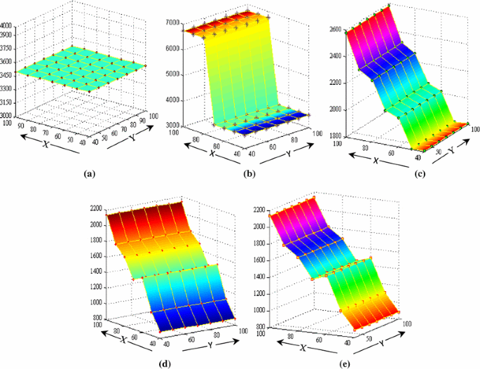

  

  Adaptability analysis of a Hilbert curve, b re-dimensioned Hilbert curve, c Delaunay triangulation, d Voronoi based algorithm, e Delaunay centroid, where X-axis represents Communication range of gateways and Y Axis represents number of gateways deployed in the target area

• b) Re-dimensioned Hilbert curve The result of this algorithm is shown in Fig. 18(b) which depicts two flat surfaces over the whole range of input parameters. Therefore, the sensitivity of the algorithm is better than the Hilbert curve but resultant path length is very longer.

• c) Delaunay triangulation The graph plotted for this algorithm [Fig. 18(c)] shows fine adaptability and the result changes very fast with the change in the input parameters. The result is also very acceptable as the path length is lesser than the Hilbert curve and re-dimensioned Hilbert curve.

• d) Voronoi vertex Here the result [Fig. 18(d)] demonstrates that the Voronoi vertex has similar properties as that of the Delaunay triangulation. It also demonstrates the sensibility and adaptability of the algorithm. It is also very effective in terms of the total distance travelled by the mobile sink in a round.

• e) Delaunay centroid The result of this proposed technique changes with the change in the network parameters. Figure 18(e) clearly witnesses its sensibility and adaptability.

8 Conclusion

In this paper, we have proposed an algorithm for constructing an efficient path of mobile sink in cluster based WSNs using Voronoi diagram. The algorithm has been designed to find a set of RPs which are efficiently selected from the Voronoi vertices in order to reduce the total path length of the mobile sink. Together with this we also have assured the complete coverage of target area so that each node can communicate with the mobile sink through one hop communication. For the fault tolerance of the proposed scheme, an efficient distributed scheme has also been developed for local recovery of orphan sensor nodes. The scheme has been experimented extensively through simulation run and the results have been compared with existing algorithms based on Hilbert curve and re-dimensioned Hilbert curve and Wang et al. algorithm. We have shown that the proposed algorithm outperform these existing schemes in terms of total path length, average waiting time, fault tolerance and adaptability. We have also shown through experiments that our scheme produces best results using Delaunay centroid. However, the proposed scheme have been shown to underperform the existing schemes in terms of energy balancing and network lifetime which may not be the much concern of quick data collection in a critical application of WSN. In our future work, an attempt will be made to design a rendezvous based path by taking care of the energy balancing of the gateways keeping the optimal coverage of the network.

References

Ren, F., Zhang, J., He, T., Lin, C., & Ren, S. K. (2011). EBRP: energy-balanced routing protocol for data gathering in wireless sensor networks. IEEE Transactions on Parallel and Distributed Systems, 22(12), 2108–2125.
Azharuddin, M., & Jana, P. K. (2016). Particle swarm optimization for maximizing lifetime of wireless sensor networks. Computers & Electrical Engineering, 51, 26–42.
Lai, Wei Kuang, Fan, Chung Shuo, & Lin, Lin Yan. (2012). Arranging cluster sizes and transmission ranges for wireless sensor networks. Information Sciences, 183, 117–131.
Ghafoor, S., Rehmani, M. H., Cho, S., & Park, S. H. (2014). An efficient trajectory design for mobile sink in a wireless sensor network. Computers & Electrical Engineering, 40(7), 2089–2100.
Gu, Y., Ji, Y., Li, J., Ren, F., & Zhao, B. (2013). EMS: Efficient mobile sink scheduling in wireless sensor networks. Ad Hoc Networks, 11(5), 1556–1570.
Garcia-Sanchez, A. J., Garcia-Sanchez, F., Losilla, F., Kulakowski, P., Garcia-Haro, J., Rodríguez, A., et al. (2010). Wireless sensor network deployment for monitoring wildlife passages. Sensors, 10(8), 7236–7262.
Salarian, H., Chin, K. W., & Naghdy, F. (2014). An energy-efficient mobile-sink path selection strategy for wireless sensor networks. IEEE Transactions on Vehicular Technology, 63(5), 2407–2419.
Samarah, S., Al-Hajri, M., & Boukerche, A. (2011). A predictive energy-efficient technique to support object-tracking sensor networks. IEEE Transactions on Vehicular Technology, 60(2), 656–663.
Ghaffari, A. (2015). Congestion control mechanisms in wireless sensor networks: A survey. Journal of Network and Computer Applications, 52, 101–115.
Anastasi, G., Conti, M., Di Francesco, M., & Passarella, A. (2009). Energy conservation in wireless sensor networks: A survey. Ad Hoc Networks, 7(3), 537–568.
Di Francesco, M., Das, S. K., & Anastasi, G. (2011). Data collection in wireless sensor networks with mobile elements: A survey. ACM Transactions on Sensor Networks (TOSN), 8(1), 7.
Johnson, D. S., & McGeoch, L. A. (2007). Experimental analysis of heuristics for the STSP. In G. Gutin & A. P. Punnen (Eds.), The traveling salesman problem and its variations (pp. 369–443). Springer US.
Yun, Y., & Xia, Y. (2010). Maximizing the lifetime of wireless sensor networks with mobile sink in delay-tolerant applications. IEEE Transactions on Mobile Computing, 9(9), 1308–1318.
Yu, L., Wang, N., & Meng, X. (2005, September). Real-time forest fire detection with wireless sensor networks. In Proceedings 2005 international conference on wireless communications, networking and mobile computing, 2005 (Vol. 2, pp. 1214–1217). IEEE.
Wang, Z. M., Melachrinoudis, E., & Basagni, S. (2005). Voronoi diagram-based linear programming modeling of wireless sensor networks with a mobile sink. In Proceedings of IIE annual conference. Institute of Industrial Engineers-Publisher.
Almi’Ani, K., Viglas, A., & Libman, L. (2010, October). Energy-efficient data gathering with tour length-constrained mobile elements in wireless sensor networks. In 2010 IEEE 35th conference on local computer networks (LCN) (pp. 582–589). IEEE.
Shah, R. C., Roy, S., Jain, S., & Brunette, W. (2003). Data mules: Modeling and analysis of a three-tier architecture for sparse sensor networks. Ad Hoc Networks, 1(2), 215–233.
Shi, Y., & Hou, Y. T. (2008, April). Theoretical results on base station movement problem for sensor network. In The 27th conference on computer communications INFOCOM 2008. IEEE.
Wang, W., Srinivasan, V., & Chua, K. C. (2005, August). Using mobile relays to prolong the lifetime of wireless sensor networks. In Proceedings of the 11th annual international conference on mobile computing and networking (pp. 270–283). ACM.
Tong, L., Zhao, Q., & Adireddy, S. (2003, October). Sensor networks with mobile agents. In Military communications conference, 2003. MILCOM’03. 2003 IEEE (Vol. 1, pp. 688–693). IEEE.
Zema, N. R., Mitton, N., & Ruggeri, G. (2014). Using location services to autonomously drive flying mobile sinks in wireless sensor networks. In N. Mitton, A. Gallais, M. Kantarci & S. Papavassiliou (Eds.), Ad hoc networks (pp. 180–191). Springer International Publishing.
Luo, J., & Hubaux, J. P. (2010). Joint sink mobility and routing to maximize the lifetime of wireless sensor networks: the case of constrained mobility. IEEE/ACM Transactions on Networking (TON), 18(3), 871–884.
Liang, W., Luo, J., & Xu, X. (2010). Prolonging network lifetime via a controlled mobile sink in wireless sensor networks. In Proceedings of Globecom’10. IEEE.
Gao, S., Zhang, H., & Das, S. K. (2011). Efficient data collection in wireless sensor networks with path-constrained mobile sinks. IEEE Transactions on Mobile Computing, 10(5), 1–9.
Xing, G., Wang, T., Xie, Z., & Jia, W. (2008). Rendezvous planning in wireless sensor networks with mobile elements. IEEE Transactions on Mobile Computing, 7(12), 1430–1443.
Mishra, M., Nitesh, K., & Jana, P. K. (2016). A delay-bound efficient path design algorithm for mobile sink in wireless sensor networks. In 2016 3rd international conference on recent advances in information technology (RAIT) (pp. 72–77). IEEE.
Komal, P., Nitesh, K., & Jana, P. K. (2016). Indegree-based path design for mobile sink in wireless sensor networks. In 2016 3rd international conference on recent advances in information technology (RAIT) (pp. 78–82). IEEE.
Kaswan, A., Nitesh, K., & Jana, P. K. (2016). A routing load balanced trajectory design for mobile sink in wireless sensor networks. In International conference on advances in computing, communications and informatics (ICACCI).
Gu, Y., Ji, Y., Li, J., & Zhao, B. (2013). ESWC: Efficient scheduling for the mobile sink in wireless sensor networks with delay constraint. IEEE Transactions on Parallel and Distributed Systems, 24(7), 1310–1320.
Marta, M., & Cardei, M. (2009). Improved sensor network lifetime with multiple mobile sinks. Pervasive and Mobile computing, 5(5), 542–555.
Yang, Y., Fonoage, M. I., & Cardei, M. (2010). Improving network lifetime with mobile wireless sensor networks. Computer Communications, 33(4), 409–419.
Xing, G., Li, M., Wang, T., Jia, W., & Huang, J. (2012). Efficient rendezvous algorithms for mobility-enabled wireless sensor networks. IEEE Transactions on Mobile Computing, 11(1), 47–60.
Preparata, F. P., Shamos, M. I., & Preparata, F. P. (1985). Computational geometry: An introduction (Vol. 5). New York: Springer.
Kuila, P., & Jana, P. K. (2014). Approximation schemes for load balanced clustering in wireless sensor networks. The Journal of Supercomputing, 68(1), 87–105.
Xu, J., Liu, W., Lang, F., Zhang, Y., & Wang, C. (2010). Distance measurement model based on RSSI in WSN. Wireless Sensor Network, 2(08), 606.
LAN/MAN Standards Committee. (2003). Part 15.4: Wireless medium access control (MAC) and physical layer (PHY) specifications for low-rate wireless personal area networks (LR-WPANs). IEEE Computer Society.
Heinzelman, W., Chandrakasan, A., & Balakrishnan, H. (2002). Application specific protocol architecture for wireless micro-sensor networks. IEEE Transactions on Wireless Communications, 1(4), 660–670.
Lee, J.-J., et al. (2008). Aging analysis in large-scale wireless sensor networks. Ad Hoc Networks, 6(7), 1117–1133.
Rausand, M., & Hoyland, A. (2004). System reliability theory: Models, statistical methods, and applications (2nd ed.). New Jersey: Wiley.
Khamsi, M. A., & Kirk, W. A. (2011). An introduction to metric spaces and fixed point theory (Vol. 53). Hoboken: Wiley.
Erlebach, T., & van Leeuwen, E. J. (2008, January). Approximating geometric coverage problems. In Proceedings of the nineteenth annual ACM-SIAM symposium on discrete algorithms (pp. 1267–1276). Society for Industrial and Applied Mathematics.
Bilò, V., Caragiannis, I., Kaklamanis, C., & Kanellopoulos, P. (2005). Geometric clustering to minimize the sum of cluster sizes. In G. S. Brodal & S. Leonardi (Eds.), Algorithms–ESA 2005 (pp. 460–471). Berlin: Springer.
Azharuddin, M., & Jana, P. K. (2016). PSO-based approach for energy-efficient and energy-balanced routing and clustering in wireless sensor networks. Soft Computing. doi:10.1007/s00500-016-2234-7.
Somasundara, A. A., Ramamoorthy, A., & Srivastava, M. B. (2007). Mobile element scheduling with dynamic deadlines. IEEE Transactions on Mobile Computing, 6(4), 395–410.
Author information
Authors and Affiliations
Corresponding author
Rights and permissions
About this article
Cite this article
Nitesh, K., Azharuddin, M. & Jana, P.K. A novel approach for designing delay efficient path for mobile sink in wireless sensor networks. Wireless Netw 24, 2337–2356 (2018). https://doi.org/10.1007/s11276-017-1477-2
Published:
Issue Date:
DOI: https://doi.org/10.1007/s11276-017-1477-2