Correlated equilibrium in a nutshell

Abstract

We analyze the concept of correlated equilibrium in the framework of two-player two-strategy games. This simple framework makes it possible to clearly demonstrate the characteristic features of this concept. We develop an intuitive and easily memorizable test for equilibrium conditions and provide a complete classification of symmetric correlated equilibria in symmetric games.

1 Introduction

Correlated equilibrium, introduced by Aumann (1974), is a classical concept in game theory. A distinctive literature has emerged to address various facets of this concept, including a multi-stage extension (Forges 1986), epistemic foundations (Aumann 1987), a direct approach to existence (Hart and Schmeidler 1989), communication mechanisms (Forges 1990), perfection-type refinements (Dhillon and Mertens 1996), emergence as limit of a class of learning dynamics (Hart and Mas-Colell 2000), and computational methods (Papadimitriou and Roughgarden 2008).

Introductory material on correlated equilibrium can be found practically in every modern text on game theory or microeconomics. Typically, the presentation of this subject is structured as follows. First a definition of this concept is given in a relatively general setting, and then the conceptual analysis proceeds nearly exclusively via examples. To the best of our knowledge, we cannot point to a source where the exposition deviates from this scheme and where a complete theory is provided, at least in a sufficiently narrow framework. The purpose of this note is to fill this gap.

As a vehicle for our analysis, we use the framework of two-player two-strategy games. It is well known that such games possess a fairly rich structure. They represent a convenient and simple model that makes it possible to clearly demonstrate a number of fundamental ideas, results and paradoxes of game theory, as reflected in the fact that some of the most widely invoked games in the social sciences belong to this class.

We begin with the definition of correlated equilibrium in a two-player two-strategy game. This notion is explained and interpreted by using Harsanyi’s (1967–1968) “mediator”. A system of linear inequalities is derived whose solutions are correlated equilibrium strategies. Then this system is transformed and represented in a compact and tractable form. Based on this representation, we develop an intuitive and easily memorizable algorithm allowing one to check whether a given correlated strategy forms a correlated equilibrium.

An outline of the algorithm is as follows. First the original game is reduced to an equivalent (having the same correlated equilibria) simple game. A game is called simple if the non-diagonal payoffs for both players are zero. After that the question boils down to the characterization of correlated equilibria for the given simple game. To analyze this question we construct an auxiliary “test game”, in which Players 1 and 2 have strategies $a_{1},a_{2}$ and $b_{1},b_{2}$, respectively. It turns out that the given correlated strategy represents a correlated equilibrium if and only if each of the strategy profiles $(a_{1},b_{1})$ and $(a_{2},b_{2})$ forms a Nash equilibrium in the test game.

We apply the above algorithm to describe all symmetric correlated equilibria in a symmetric simple two-strategy game. In this narrow, but still interesting, framework a correlated strategy can be specified by two numbers and thus can be represented by a point on the plane. Several cases are considered in which the set of correlated equilibria corresponds to a quadrangle, triangle, or segment in the plane. This leads to a complete theory of symmetric correlated equilibria in the simplest model we are dealing with.

In the authors’ mind, the main motivation behind this novel treatment of correlated equilibrium is twofold. First, it may pave the way for a more extensive use of correlated equilibrium in applied settings in economics and other social sciences. Second, it may facilitate the teaching of this concept at a level beyond illustrative examples.

The remainder of the paper is organized as follows. In Sect. 2, we introduce the concept of correlated equilibrium and derive the system of linear inequalities characterizing all correlated equilibria. In Sect. 3, we develop an algorithm based on the “test game” making it possible to verify that a given correlated strategy forms a correlated equilibrium. In Sect. 4, we provide a complete characterization of all symmetric correlated equilibria for a symmetric simple two-strategy game. An example in Sect. 5 concludes the paper.

2 Correlated strategies and correlated equilibrium

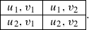
Consider a two-player two-strategy game with strategy sets $A=\{a_{1},a_{2} \}$, $B=\{b_{1},b_{2}\}$ and payoff functions u(a, b), v(a, b). A correlated strategy

$$\begin{aligned} \gamma =\left( \begin{array} [c]{cc} \gamma _{11} &{} \gamma _{12}\\ \gamma _{21} &{} \gamma _{22} \end{array} \right) ,\ \gamma _{ij}\ge 0,\ \sum _{i,j=1,2}\gamma _{ij}=1, \end{aligned}$$

(1)

is a probability distribution on the set of strategy profiles $(a_{i},b_{j})$ of the two players. The number $\gamma _{ij}$ is the probability that the randomly chosen strategy profile (a, b) of the players is $(a_{i},b_{j})$:

$$\begin{aligned} \gamma _{ij}=\Pr \{(a,b)=(a_{i},b_{j})\}. \end{aligned}$$

A correlated strategy may be regarded as a randomized plan of coordinated actions of both players, which is performed by using communication (involving, for example, a “mediator”).

For the correlated strategy $\gamma$, the expectations of the payoffs u(a, b) and v(a, b) are given by

$$\begin{aligned} u(\gamma )=Eu(a,b)=\sum _{i,j=1,2}\gamma _{ij}u(a_{i},b_{j}),\;v(\gamma )=Ev(a,b)=\sum _{i,j=1,2}\gamma _{ij}v(a_{i},b_{j}). \end{aligned}$$

Consider the framework for analyzing correlated strategies involving a mediator due to Harsanyi (1967–1968). Suppose the players use some correlated strategy $\gamma$ defined by probabilities $\gamma _{11}$, $\gamma _{12}$, $\gamma _{21}$, and $\gamma _{22}$. Let us imagine that there is a mediator selecting the strategy profile (a, b) at random according to the probabilities $\gamma _{ij}$, so that $\gamma _{ij}=\Pr \{(a,b)=(a_{i},b_{j})\}$. If the random strategy profile (a, b) happens to be $(a_{i},b_{j})$, the mediator recommends Player 1 to play $a_{i}$ and Player 2 to play $b_{j}$. The mediator communicates $a_{i}$ (only) to Player 1 and $b_{j}$ (only) to Player 2 and each player does not know what has been recommended to the other.

For our further analysis, we will need to consider the conditional expectations:

$$\begin{aligned} E[u(a^{\prime },b)|a=a_{i}]\; \text {and}\; E[v(a,b^{\prime })|b=b_{j}] \end{aligned}$$

(2)

for any $a^{\prime }\in A$ and $b^{\prime }\in B$. In the former expectation, $a^{\prime }$ and $a=a_{i}$ are fixed, and b is random. The expectation is taken under the conditional distribution of b given $a=a_{i}$. In the latter expectation, $b^{\prime }$ and $b=b_{j}$ are fixed, and a is random. The expectation is taken under the conditional distribution of a given $b=b_{j}$ .

Let us explain the meaning of the conditional expectations (2), say, the former. Suppose the mediator has announced $a_{i}$ to Player 1, i.e., the event $\{a=a_{i}\}$ has occurred. Assume that for one reason or another, Player 1 decides to disobey the mediator’s recommendation and to play another strategy $a^{\prime }$, not $a_{i}$. Then the expected payoff Player 1 gets (provided that Player 2 obeys the recommendations of the mediator) is the conditional expectation $E[u(a^{\prime },b)|a=a_{i}]$. The conditional expectation $E[v(a,b^{\prime })|b=b_{j}]$ has the analogous meaning.

A correlated strategy $\gamma$ is said to form a correlated equilibrium if

$$\begin{aligned} E[u(a_{i},b)|a= & {} a_{i}]\ge E[u(a^{\prime },b)|a=a_{i}]\text { for all }i \text { and }a^{\prime }{;} \end{aligned}$$

(3)

$$\begin{aligned} E[v(a,b_{j})|b= & {} b_{j}]\ge E[v(a,b^{\prime })|b=b_{j}]\text { for all }j\text { and }b^{\prime }{.} \end{aligned}$$

(4)

Conditions (3) and (4)—termed strategic incentive constraints—say that in the correlated equilibrium, it is optimal for each player to obey the mediator’s recommendations. Condition (3) states that, given $a=a_{i}$, the maximum conditional expected payoff of Player 1 is attained when he plays $a_{i}$. Analogously, given $b=b_{j}$, the maximum expected payoff of Player 2 is attained when she plays $b_{j}$. In this sense, the equilibrium correlated strategy $\gamma$ is self-enforcing.

Denote by $\mu _{ij}$ the conditional probability that $a=a_{i}$ given $b=b_{j}$ and by $\nu _{ji}$ the conditional probability that $b=b_{j}$ given $a=a_{i}$. Then

$$\begin{aligned} \mu _{ij}=\Pr \{a=a_{i}|b=b_{j}\}=\frac{\Pr \{a=a_{i}, b=b_{j}\}}{\Pr \{b=b_{j} \}}=\frac{\gamma _{ij}}{\gamma _{1j}+\gamma _{2j}} \end{aligned}$$

and

$$\begin{aligned} \nu _{ji}=\Pr \{b=b_{j}|a=a_{i}\}=\frac{\Pr \{b=b_{j}, a=a_{i}\}}{\Pr \{a=a_{i} \}}=\frac{\gamma _{ij}}{\gamma _{i1}+\gamma _{i2}}. \end{aligned}$$

(5)

It is convenient to write conditions (3) and (4) in the following form:

$$\begin{aligned} E[u(a_{i},b)-u(a^{\prime },b)|a= & {} a_{i}]\ge 0 \text { for all }i \text { and }a^{\prime }\ne a_{i}, \\ E[v(a,b_{j})-v(a,b^{\prime })|b= & {} b_{j}]\ge 0 \text { for all }j \text { and }b^{\prime }\ne b_{j}. \end{aligned}$$

Express the conditional expectations through conditional probabilities (5) and multiply the first inequality by $\gamma _{i1} +\gamma _{i2}$ and the second by $\gamma _{1j}+\gamma _{2j}$. This yields

$$\begin{aligned}{}[u(a_{i},b_{1})-u(a^{\prime },b_{1})]\gamma _{1i}+[u(a_{i},b_{2} )-u(a^{\prime },b_{2})]\gamma _{2i}\ge & {} 0, \end{aligned}$$

(6)

$$\begin{aligned}{}[v(a_{1},b_{j})-v(a_{1},b^{\prime })]\gamma _{1j}+[v(a_{2},b_{j} )-v(a_{2},b^{\prime })]\mu _{2j}\ge & {} 0. \end{aligned}$$

(7)

3 Correlated equilibrium test

Let us introduce the notation:

$$\begin{aligned} u_{ij}=u(a_{i},b_{j}),\ v_{ij}=v(a_{i},b_{j}),\ a^{\prime }=a_{k},\ b^{\prime }=b_{m}. \end{aligned}$$

Then inequalities (6) and (7) can be written for all $i,k\ne i$ and $j,m\ne j$ as

$$\begin{aligned} (u_{i1}-u_{k1})\gamma _{i1}+(u_{i2}-u_{k2})\gamma _{i2}\ge 0,\ (v_{1j} -v_{1m})\gamma _{1j}+(v_{2j}-v_{2m})\gamma _{2j}\ge 0. \qquad \end{aligned}$$

(8)

A correlated strategy $\gamma =(\gamma _{ij})$ forms a correlated equilibrium in a game with payoffs $u_{ij}=u(a_{i},b_{j})$, $v_{ij} =v(a_{i},b_{j})$ if and only if the four inequalities in (8) hold.

From (8), we recover directly the well-known result that the set of correlated equilibria is a compact and convex set (Myerson 1991).

Consider a new game, called the reduced version of the original one, in which the payoff matrix is

It has zero non-diagonal payoffs. Such games are called simple. Observe that conditions (8) for the original game and for its reduced version coincide. Hence both games have the same correlated equilibria!

Let us examine correlated equilibria in a simple game

(9)

For such games, conditions (8) characterizing correlated equilibria take on the following form

(10)

Consider the following auxiliary game, which will be called the test game:

(11)

Proposition

The correlated strategy $\gamma =(\gamma _{ij} )$ forms a correlated equilibrium in the simple game (9) if and only if the strategy profiles $(a_{1},b_{1})$ and $(a_{2},b_{2})$ form Nash equilibria in the test game.

Proof

To prove the proposition, observe that

• (I) holds if and only if $a_{1}$ is the best response to $b_{1}$;

• (II) holds if and only if $a_{2}$ is the best response to $b_{2};$

• (III) holds if and only if $b_{1}$ is the best response to $a_{1};$

• (IV) holds if and only if $b_{2}$ is the best response to $a_{2}.$

Let us describe an easily memorizable algorithm for constructing the test game. Suppose we are given a simple game and a correlated strategy

1st step :

Based on the former matrix, construct the following one

2nd step :

Transpose the matrix $\gamma$, i.e., swap $\gamma _{12}$ and $\gamma _{21}$:

$$\begin{aligned} \left( \begin{array} [c]{cc} \gamma _{11} &{}\quad \gamma _{21}\\ \gamma _{12} &{}\quad \gamma _{22} \end{array} \right) . \end{aligned}$$

3rd step :

Multiply element-wise the last two matrices:

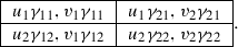
The result is precisely the payoff matrix for the test game!

The above analysis leads to the following procedure for the verification that some given correlated strategy $\gamma$ forms a correlated equilibrium. (1) Reduce the given game to a simple one. (2) Construct the test game. (3) Check whether each of the strategy profiles $(a_{1},b_{1})$ and $(a_{2},b_{2})$ forms a Nash equilibrium. If the answer to the last question is positive, then $\gamma$ is indeed a correlated equilibrium. If either $(a_{1},b_{1})$ or $(a_{2},b_{2})$ is not a Nash equilibrium, then $\gamma$ is not a correlated equilibrium.

Consider an example. Let us verify that the correlated strategy

$$\begin{aligned} \gamma =\left( \begin{array} [c]{cc} \gamma _{11}=1/3 &{} \gamma _{12}=0\\ \gamma _{21}=1/3 &{} \gamma _{22}=1/3 \end{array} \right) \end{aligned}$$

(12)

forms a correlated equilibrium in the game

The reduced simple game is as follows:

The test game (constructed by using the above algorithm) has the following payoff matrix:

Both $(a_{1},b_{1})$ and $(a_{2},b_{2})$ are Nash equilibria, consequently, the correlated strategy (12) indeed forms a correlated equilibrium in the given game. $\square$

4 Symmetric correlated equilibria in symmetric games

For a symmetric game, $v(a,b)=u(b,a)$ for all a, b, i.e., in our notation, $v_{ij}=u_{ji},\ i,j=1,2.$ If the original game

is symmetric, then so is the reduced one:

A correlated strategy $\gamma$ is called symmetric if the matrix $\gamma$ is symmetric: $\gamma _{12}=\gamma _{21}$. Consider a simple symmetric game

(13)

(we write only the payoffs of the first player). If a correlated strategy $\gamma =(\gamma _{ij})$ is symmetric, then the four conditions (10) hold if and only if (I) and (II) hold (conditions (III) and (IV) coincide with (I) and (II) because $u_{1}=v_{1}$, $u_{2}=v_{2}$ and $\gamma _{12}=\gamma _{21}$).

Our next goal is to characterize symmetric correlated equilibria in simple symmetric games (13).

For symmetric correlated strategies $\gamma$, it will be convenient to use the following notation

$$\begin{aligned} \gamma =\left( \begin{array} [c]{cc} \rho _{1} &{} \theta \\ \theta &{} \rho _{2} \end{array} \right) , \ \rho _{1}\ge 0, \ \rho _{2}\ge 0, \ \theta \ge 0, \ \rho _{1}+\rho _{2}+2\theta =1, \end{aligned}$$

(14)

where $\rho _{1}=\gamma _{11},\rho _{2}=\gamma _{22}$ and $\theta =\gamma _{12}=\gamma _{21}$.

For a simple game (13) and a symmetric correlated strategy (14), the test game is also symmetric and it takes on the following form:

(15)

Conditions (I) and (II) mean that a symmetric correlated strategy $\gamma$ forms a correlated equilibrium if and only if both $(a_{1},a_{1})$ and $(a_{2},a_{2})$ are Nash equilibria in the test game, i.e.,

$$\begin{aligned} \text {(I)}\ u_{1}\rho _{1}\ge u_{2}\theta ,\text { (II)}\ u_{2}\rho _{2}\ge u_{1}\theta . \end{aligned}$$

(16)

For a simple symmetric game (13) and a symmetric correlated strategy (14), we can express $\theta$ as

$$\begin{aligned} \theta =(1-\rho _{1}-\rho _{2})/2. \end{aligned}$$

Then conditions (16) can be written as

$$\begin{aligned} \rho _{1}\left( 2u_{1}+u_{2}\right) +\rho _{2}u_{2}\ge u_{2}, \ \rho _{1} u_{1}+\rho _{2}\left( 2u_{2}+u_{1}\right) \ge u_{1}. \end{aligned}$$

(17)

Thus a correlated strategy (14) forms a correlated equilibrium if and only if the pair of non-negative numbers $(\rho _{1},\rho _{2})$ satisfies the system of linear inequalities (17) and

$$\begin{aligned} \rho _{1}+\rho _{2}\le 1. \end{aligned}$$

Let us describe the set of such pairs of numbers $(\rho _{1},\rho _{2})$, representing them as points on the plane. Without loss of generality, we shall assume that $u_{1}\ge u_{2}$.

Case 1 $u_{1}\ge u_{2}>0$. In this case, inequalities (17) are equivalent to the following ones:

$$\begin{aligned} \frac{\rho _{1}}{U_{2}}+\rho _{2}\ge 1, \ \rho _{1}+\frac{\rho _{2}}{U_{1} }\ge 1, \end{aligned}$$

where

$$\begin{aligned} U_{1}=\frac{u_{1}}{u_{1}+2u_{2}}, \ U_{2}=\frac{u_{2}}{2u_{1}+u_{2}}. \end{aligned}$$

The set of points $(\rho _{1},\rho _{2})$ with $\rho _{1}\ge 0$, $\rho _{2}\ge 0$ satisfying these inequalities and $\rho _{1}+\rho _{2}\le 1$ is the triangle $C^{E}$; see Fig. 1.

Fig. 1

Case 1: triangle

Case 2 $0>u_{1}\ge u_{2}$. Then inequalities (17) can be transformed to the following ones:

$$\begin{aligned} \frac{\rho _{1}}{U_{2}}+\rho _{2}\le 1, \ \rho _{1}+\frac{\rho _{2}}{U_{1} }\le 1, \end{aligned}$$

(18)

where

$$\begin{aligned} U_{1}=\frac{u_{1}}{u_{1}+2u_{2}},\ U_{2}=\frac{u_{2}}{2u_{1}+u_{2}}. \end{aligned}$$

The set of points $(\rho _{1},\rho _{2})$ with $\rho _{1}\ge 0$, $\rho _{2}\ge 0$ satisfying these inequalities is the quadrangle $C^{E}$; see Fig. 2.

Fig. 2

Case 2: quadrangle

Note that the inequality $\rho _{1}+\rho _{2}\le 1$ follows automatically from each of the above two inequalities because $0<U_{2}<1$ and $0<U_{1}<1$.

Case 3 $u_{1}>0>u_{2}$. Then the first of the equilibrium conditions (16) is always satisfied. From the second condition, it follows that $u_{2}\rho _{2}=u_{1}\theta =0$. Thus

$$\begin{aligned} \rho _{2}=\theta =0, \ \rho _{1}=1, \end{aligned}$$

and so in this case the correlated equilibrium is given by

$$\begin{aligned} \gamma =\left( \begin{array} [c]{cc} 1 &{}\quad 0\\ 0 &{}\quad 0 \end{array} \right) , \end{aligned}$$

which is nothing but a symmetric pure strategy Nash equilibrium $(a_{1} ,a_{1})$ where both players play the strategy $a_{1}$.

Case 4 $u_{1}>u_{2}=0$. Condition (II) in (16) can be written as $0=u_{2}\rho _{2}\ge u_{1}\theta \ge 0$, from which we find that $\theta =0$. The second condition is always satisfied, and so the set of correlated equilibria is given by

$$\begin{aligned} \gamma =\left( \begin{array} [c]{cc} \rho _{1} &{} 0\\ 0 &{} 1-\rho _{1} \end{array} \right) , \ 0\le \rho _{1}\le 1. \end{aligned}$$

This is the segment connecting the points $\left( 1,0\right)$ and $\left( 0,1\right)$ in the $\left( \rho _{1},\rho _{2}\right)$-plane.

Case 5 $u_{1}=0>u_{2}$. Condition (I) in (16) is always satisfied. From (II) it follows that $0\ge u_{2}\rho _{2}\ge u_{1}\theta =0$, from which we find that $\rho _{2}=0$. Thus in this case, $0\le \rho _{1}\le 1$, $\theta =(1-\rho _{1})/2$ and $\rho _{2}=0$. Consequently, the set of correlated equilibria consists of correlated strategies of the form

$$\begin{aligned} \gamma =\left( \begin{array} [c]{cc} \rho _{1} &{} \left( 1-\rho _{1}\right) /2\\ \left( 1-\rho _{1}\right) /2 &{} 0 \end{array} \right) , \ 0\le \rho _{1}\le 1. \end{aligned}$$

This set is represented by the line segment connecting the points $\left( 0,0\right)$ and $\left( 1,0\right)$ in the $\left( \rho _{1},\rho _{2}\right)$-plane.

Case 6 $u_{1}=u_{2}=0$. In this case any strategy (14) with $\left( \rho _{1},\rho _{2}\right)$ from the triangle $\left\{ \left( \rho _{1},\rho _{2}\right) :\rho _{1}\ge 0,\ \rho _{2}\ge 0, \ \rho _{1}+\rho _{2}\le 1\right\}$ forms a correlated equilibrium.

5 Example

Let us apply the above considerations to the analysis of a classical example: the “chicken game”. This is a symmetric game where each player has two strategies $a_{1}$ “dare” and $a_{2}$ “chicken out”. The payoff matrix is as follows:

We construct the reduced symmetric game (non-diagonal elements are subtracted from columns):

Here, $u_{1}<0$, $u_{2}<0$, and so we are in the framework of case 2. We have

$$\begin{aligned} U_{1}=\frac{u_{1}}{u_{1}+2u_{2}}=\frac{1}{2}\text { and }U_{2}=\frac{u_{2} }{2u_{1}+u_{2}}=\frac{1}{5}. \end{aligned}$$

By virtue of the results obtained, symmetric correlated equilibria (13) in this game correspond to those and only those pairs of non-negative numbers $(\rho _{1},\rho _{2})$ that satisfy

$$\begin{aligned} 5\rho _{1}+\rho _{2}\le 1,\ \rho _{1}+2\rho _{2}\le 1 \end{aligned}$$

(19)

[see (18)]. Geometrically, the set $C^{E}$ of points $(\rho _{1} ,\rho _{2})\ge 0$ in the plane satisfying (19) is a quadrangle; see Fig. 3.

Fig. 3

Example

In the game at hand, the expected payoff for the correlated strategy (13) can be computed as follows:

$$\begin{aligned} u(\gamma )=6\rho _{2}+9\theta =\frac{3}{2}(3-3\rho _{1}+\rho _{2}). \end{aligned}$$

It is of interest to examine which of the symmetric correlated equilibria maximizes the expected payoff of each player. Maximizing this function on the quadrangle $C^{E}$ is equivalent to maximizing $z=\rho _{2}-3\rho _{1}$ on $C^{E}$. The analysis of the diagram in Fig. 3 (the dotted lines are level sets of the function z) shows that the maximum is attained at $(\rho _{1},\rho _{2})=(0,1/2)$, for which

$$\begin{aligned} \gamma =\left( \begin{array} [c]{cc} 0 &{}\quad 1/4\\ 1/4 &{}\quad 1/2 \end{array} \right) \end{aligned}$$

and $u(\gamma )=5\frac{1}{4}$.

This game does not have any symmetric pure strategy Nash equilibrium, but it has a unique symmetric mixed strategy Nash equilibrium, in which the players select $a_{1}$ and $a_{2}$ with probabilities 1 / 3 and 2 / 3 and the expected payoff of each player is $4\frac{1}{3}$. We can see that the correlated equilibrium described above yields a tangibly larger payoff of $5\frac{1}{4}$.

It is well known that Nash equilibria are quite often inefficient. An equilibrium might be a compromise, the achievement of which entails substantial losses to all the players. A correlated equilibrium makes it possible, by invoking a mediator, to reduce these losses. This illustrates in a game-theoretic setting the potential efficiency of intermediaries in resolving conflicts of interest.

References

Aumann, R. (1974). Subjectivity and correlation in randomized strategies. Journal of Mathematical Economics, 1, 67–96.
Aumann, R. (1987). Correlated equilibrium as an expression of Bayesian rationality. Econometrica, 55, 1–18.
Dhillon, A., & Mertens, J.-F. (1996). Perfect correlated equilibria. Journal of Economic Theory, 68, 279–302.
Forges, F. (1986). An approach to communication equilibria. Econometrica, 54, 1375–1385.
Forges, F. (1990). Universal mechanisms. Econometrica, 58, 1341–1364.
Harsanyi, J.C. (1967–1968). Games with incomplete information played by ’Bayesian’ players. Management Science, 14, Parts I–III, 159–182, 320–334 and 486–502.
Hart, S., & Mas-Colell, A. (2000). A simple adaptive procedure leading to correlated equilibria. Econometrica, 68, 1127–1150.
Hart, S., & Schmeidler, D. (1989). Existence of correlated equilibria. Mathematics of Operations Research, 14, 18–25.
Myerson, R. (1991). Game theory. Cambridge: Harvard University Press.
Papadimitriou, C., & Roughgarden, T. (2008). Computing correlated equilibria in multi-player games. Journal of the ACM, 55(3), 1–29 (article 14).
Author information
Authors and Affiliations
Corresponding author
Rights and permissions
About this article
Cite this article
Amir, R., Belkov, S. & Evstigneev, I.V. Correlated equilibrium in a nutshell. Theory Decis 83, 457–468 (2017). https://doi.org/10.1007/s11238-017-9609-9
Published:
Issue Date:
DOI: https://doi.org/10.1007/s11238-017-9609-9