LASCO-C3 Observations of the K- and F-Coronae over 24 Years (1996 – 2019): Photopolarimetry and Electron Density Distribution

Abstract

We present the polarimetric analysis of the white-light images of the corona obtained with the Large-Angle Spectrometric COronagraph LASCO-C3 onboard the Solar and Heliospheric Observatory (SOHO) from 1996 to 2019, leading to the separation of the K- and F-components and the derivation of the electron-density distribution. The analysis makes use of polarized sequences composed of three images obtained through three polarizers oriented at $+60^{\circ}$, $0^{\circ}$, and $-60^{\circ }$, complemented by a neighboring unpolarized image. However, the degradation of the $0^{\circ}$ polarizer noticed in 1999 compelled us to reconstruct the corresponding images from those obtained with the two other polarizers and the unpolarized ones thereafter. The analysis closely follows the method developed for LASCO-C2 (Lamy et al. in Solar Phys. 295, 89, 2020) and implements the formalism of Mueller, albeit with additional difficulties notably the presence of a non-axially symmetric component of stray light. Critical corrections were derived from a SOHO roll sequence and from consistency criteria (e.g. the “tangential” direction of polarization). The quasi-uninterrupted photopolarimetric analysis of the outer corona over two complete Solar Cycles 23 and 24 was successfully achieved and our final results encompass the characterization of its polarization, of its polarized radiance, of the two-dimensional electron density, and of the K-corona. Comparison between the C3 and C2 results in the region where their fields of view overlap shows an overall agreement. The C3 results are further in agreement with those of eclipses and radio-ranging measurements to an elongation of ≈10 R_⊙ but tend to diverge further out. Although the coronal polarization out to 20 R_⊙ is still highly correlated with the temporal variation of the total magnetic field, this divergence probably results from the increasing polarization of the F-corona with increasing solar elongation.

1 Introduction

Whereas the observation of the inner solar corona (defined here as extending to ≈3 R_⊙ from the center of the solar disk) in polarized white-light has been actively pursued for decades with different purposes as summarized by Lamy et al. (2020), the outer corona has received far less attention. This is readily explained by the faintness of the brightness and of the polarization compared with the inner region, so that stray-light components (stray light from the instrument and from the Earth’s atmosphere in the case of ground-based eclipse observations) become a major concern. Ground-based coronagraphs even located at high altitude such as the Mark III, Mark IV, and K-Cor at the Mauna Loa Solar Observatory (Hawaii) have not helped as their polarized brightness $pB$-measurements are limited to a typical elongation of ≈1.5 R_⊙ from the center of the Sun. The space coronagraphs of the first generation such as that flown onboard the Orbiting Solar Observatory (OSO)-7 (Koomen et al., 1975) and the Solar Maximum Mission (SMM) Coronagraph/Polarimeter (MacQueen et al., 1980) were hampered by the poor radiometric performances of their vidicon detectors. More recent space instruments obtained very valuable white-light images of the outer corona, notably the star-tracker camera of the Clementine spacecraft over elongations of $3^{\circ}\lesssim\epsilon\lesssim30^{\circ}$ (Hahn et al., 2002) and the Solar Terrestrial Relationships Observatory (STEREO) Sun–Earth Connection Coronal and Heliospheric Investigation (SECCHI/HI-1) heliospheric imager over elongations of $5^{\circ}\lesssim\epsilon\lesssim24^{\circ}$ (Stenborg, Howard, and Stauffer, 2018) but they had no polarimetric capability.

We are therefore left with the eclipse measurements performed in the years 1952 – 1973 as presented in the review article of Koutchmy and Lamy (1985). Table 1 summarizes the information relevant to the six campaigns that took place during this time interval. In comparison with Figure 4 of Koutchmy and Lamy (1985), we include the results of Michard et al. (1954) but disregard those of Pepin (1970) since this author displays a map of only a few contours of constant polarization (his Figure 3) from which it is retrospectively difficult to construct reliable equatorial and polar profiles. With the exception of the results of Michard and Sotirovski (1965), all other profiles along the equatorial direction agree on a continuous decrease from ≈0.18 at 3 R_⊙ to ≈0.08 at 6 R_⊙. They diverge beyond, an effect that Koutchmy and Lamy (1985) attributed possibly to the presence or absence of a window in aircraft observations. The polarization along the polar direction is much fainter and the bulk of the measurements do not go beyond 5 R_⊙.

Table 1 Summary of past results on the polarization of the outer corona along the equatorial and polar directions.

Whereas the polarization in the inner corona is determined by the K-component, in the outer corona it depends upon the interplay of the K- and F-components according to their respective weight as the elongation increases. This implies that, at some elongation, there must be a turnover from an inner region where the polarization is dominated by the K-component to an outer region where it is dominated by the F-component according to the following equation:

$$ p= \frac{p_{\scriptscriptstyle\mathrm{K}}\,B_{\scriptscriptstyle \mathrm{K}}+p_{\scriptscriptstyle\mathrm{F}}\,B_{\scriptscriptstyle \mathrm{F}}}{B_{\scriptscriptstyle\mathrm{K}}+B_{\scriptscriptstyle \mathrm{F}}} $$

(1)

and connecting to the zodiacal light further out. In other words, we expect the radial variation of the polarization of the corona to slowly decrease with increasing elongation and then rise to progressively match the classical values of the zodiacal light at elongations $\epsilon\geq30^{\circ}$; see for instance Figure 8 c of Lamy and Perrin (1986). In between, there are presently only two measurements from the rocket flight of Leinert, Link, and Pitz (1974) corrected by Leinert et al. (1976): $p=0.137$ at $\epsilon=14.3^{\circ}$ (55 R_⊙) and $p=0.155$ at $\epsilon=21.0^{\circ}$ (82.5 R_⊙). Figure 1 is intended to offer a view of this situation. It regroups the above result of Leinert et al. (1976), the polarization of an homogeneous, minimum K+F-corona between 5 and 20 R_⊙ compiled in Allen’s Astrophysical Quantities (Cox, 2015), and the model of the outer corona constructed by Blackwell and Petford (1966), which we briefly summarize. The K/F-separation was achieved based on measurements of the depth of the H$\alpha$ absorption line in the spectrum of the corona to an elongation of 16 R_⊙ and the resulting radial profile of the K-corona along the equatorial direction was inverted to yield a profile of the electron density, which was subsequently smoothly extrapolated to 1 AU. This latter profile was then used to calculate the brightness and polarization of the K-corona. Combining with values of the K+F-brightness from eclipse observations complemented by zodiacal-light data, Blackwell and Petford (1966) were able to obtain the radial variations of the brightness and the polarization of the K-, F-, and K+F-coronae between 5 and 40 R_⊙ (their Table III). An extrapolation of the K+F-polarization curve of Blackwell and Petford (1966) suggests a reasonable connection with the value of Leinert et al. (1976) at 82.5 R_⊙ whereas that at 55 R_⊙ is probably incorrect (quasi-identical polarization values at such different elongations are extremely unlikely). This model predicts i) a polarization of the F-corona remaining extremely low (less than 0.01) up to ≈20 R_⊙, and ii) a leveling-off of the total polarization $p$ followed by a turnover starting at about 30 R_⊙. In reality, the location of this turnover depends upon several factors, primarily the activity of the Sun, which directly influences the radiance and the geometry of the K-corona. As a matter of fact, the photometers at 16^∘ to the ecliptic plane onboard the Helios spacecraft detected variations of the polarization of the zodiacal light correlated with solar activity, prominently in the polar regions (Leinert and Pitz, 1989). The eclipse results listed in Table 1 will be further illustrated and discussed when we compare them with those coming from the LASCO-C3 observations.

Figure 1

Polarization of the K+F and F coronae as a function of solar elongation in the equatorial direction from different sources. The “Blackwell” K+F and F data are from Blackwell and Petford (1966). The “SK” data are the compilation of two sources, Saito, Hata, and Tojo (1972) and Koutchmy, Picat, and Dantel (1977) presented by S. Koutchmy in Section 14.8 “Corona” of the Fourth Edition of Allen’s Astrophysical Quantities (Cox, 2015). Additional values for the zodiacal light are from Leinert et al. (1976). The broken line represents the linear interpolation (on the log–log scale) between the data of Blackwell and Petford (1966) and the second value of Leinert et al. (1976) at 82.5 R_⊙.

The Large-Angle Spectrometric COronagraph (LASCO), a set of three coronagraphs (Brueckner et al., 1995) onboard the Solar and Heliospheric Observatory (SOHO) opened an entirely new era in the domain of photometric and polarimetric investigations of the white-light corona. LASCO-C3, one of the two externally occulted coronagraphs of direct interest to this present article, has been in nearly continuous operation since January 1996, recording the solar corona from 3.7 to 30 R_⊙ in unpolarized and polarized light implementing the same system as LASCO-C2: a set of three polarizers oriented at $+60^{\circ}$, $0^{\circ}$, $-60^{\circ }$ mounted on a wheel. In spite of this potential and of the limited knowledge of the outer corona, these C3 data have not received particular attention. Encouraged by our achievements with the C2 data as described by Lamy et al. (2020) (hereafter Article I), we decided to analyze the C3 polarization data. Since we implement the same technique, we limit its presentation here to a summary and refer the interested reader to the aforementioned article for background information on the coronal polarization and for detail of the analysis.

Our article is organized as follows: Section 2 describes the observations and the processing of the data. Section 3 presents the method of polarization analysis based on the Mueller formalism, the determination of the Mueller matrices, and the calibration of the instrument. The practical implementation of the analysis, the initial results, and critical tests then reveals the necessity of additional corrections, which are dealt with in Section 4. Final results for the polarization, the polarized radiance [$pB$], the electron density, and the radiance of the K-corona over 24 years are presented in Section 5, and uncertainties are discussed in Section 6. These results are subsequently compared with those coming from LASCO-C2 (Section 7), solar eclipses (Sections 8 and 9), and radio-ranging measurements in Section 10. Finally, we conclude in Section 11.

2 LASCO-C3 Observations and Data Processing

2.1 Observations

A LASCO polarization sequence is composed of three polarized images of the corona successively obtained with three polarizers oriented at +60^∘, 0^∘, and −60^∘ with respect to the direction of the rows (${{x}}$-axis) of the CCD detector and an unpolarized image altogether forming a quadruplet. The polarizers themselves are a sandwich of a Polaroid foil (Kodak HN22) cemented between two polished glass plates. The polarization sequences are prominently taken with the “orange” filter (bandpass of 540 – 640 nm) in the binned format of 512×512 pixels in order to improve the signal-to-noise ratio of the polarized images. A few sequences were taken in the full format of 1024×1024 pixels and were subsequently rebinned to 512×512 pixels.

Figure 2 displays the chronogram of the polarization sequences, typically one per day. This routine program was affected by two major interruptions due to: i) the accidental loss of SOHO during a roll maneuver on 25 June 1998, which resulted in a long data gap until recovery on 22 October 1998, and ii) the failure of the gyroscopes, which caused another gap from 21 December 1998 to 6 February 1999 when nominal operation resumed. Special polarization sequences took place a few times as shown by the peaks in the chronogram. During its first years of operation, the attitude of SOHO was set such that its reference axis was aligned along the sky-projected direction of the solar rotational axis resulting in this direction being “vertical” (i.e. along the column or ${{y}}$-axis of the CCD detector) with solar north up on the LASCO images. Starting on 10 July 2013 and following the failure of the motor steering its antenna, SOHO was periodically (every three months) rolled by 180^∘ to maximize telemetry transmission to Earth. On 29 October 2010 and still on-going, the attitude of SOHO was changed to simplify operation, the reference orientation being fixed to the perpendicular to the ecliptic plane causing the projected direction of the solar rotational axis to oscillate between ±7^∘ 15’ around the “vertical” direction on the LASCO images.

Figure 2

Monthly averaged daily rate of the polarization sequences obtained with the LASCO-C3 coronagraph with the orange filter in the binned format of 512×512 pixels. The arrow indicates the roll sequence of the spacecraft used for calibration.

2.2 Preprocessing of the C3 Images

The original data stream coming from the spacecraft represents the lowest level data, known as Level-0. As explained in Article I, they were processed by the LASCO team at the Naval Research Laboratory to produce FITS files with documented headers forming the Level-0.5 data set of individual images; no correction was applied at this stage. This process was slowed down in 2015 and eventually terminated. As a consequence, we decided in October 2015 to switch to the “quick look data” produced at the Goddard Space Flight Center. Strictly speaking, these two data sets Level-0.5 and “quick look” are identical except for slightly fewer missing telemetry blocks in the former data set.

The LASCO team at the Laboratoire d’Astrophysique de Marseille (formerly Laboratoire d’Astronomie Spatiale) developed a two-stage procedure that corrects for all instrumental effects and processes the raw data to scientific images of the corona. The first stage consists in a preprocessing applied to all images as described in our past articles, in particular Article I. In summary, it performs bias correction, exposure-time equalization (Llebaria and Thernisien, 2001), and corrects for missing blocks and cosmic-ray impacts (Pagot et al., 2014); see Article I for details. The second stage is applied to the polarization sequences and is described in the next section.

2.3 Processing of the C3 Polarized Images

The polarized images further undergo the following processes:

• i) Rebinning to 512×512 pixels. In practice, this applies to the few 1024×1024 pixels images to bring them to a common format for polarization analysis.

• ii) Correction for the stray-light ramp. Unlike C2, C3 is affected by a non-axially symmetric stray-light pattern best defined as a ramp roughly aligned with the NW–SE diagonal of the square field of view. This effect was thoroughly investigated by Morrill et al. (2006), who conjectured that it most likely results from a reflection from the CCD surface. We did not make use of the map of the ramp that they determined (their Figure 20) as we later realized that their determination suffers from a flaw that led us to re-consider the problem and look for a correct solution. This is described in detail in the Appendix.

• iii) Polarimetric analysis based on the Mueller formalism. It is applied to each triplet of polarized images and returns images of the total radiance, the polarized radiance, the polarization, and the angle of polarization.

• iv) Vignetting correction. This vignetting introduced by the occulters is removed from the radiance images using a geometric model of the two-dimensional vignetting function of C3 (Llebaria, Lamy, and Bout, 2004). It is further combined with a cos$^{4}(\phi)$ correction for the optical vignetting where $\phi$ is the incidence angle of any light ray in the field of view as measured from the optical axis.

• v) Absolute calibration of the total radiance derived from the photometric measurements of stars present in the C3 field of view (Thernisien et al., 2006).

• vi) K/F-separation.

3 Analysis of the LASCO-C3 Polarized Images

We strictly follow the method implemented in Article I for the analysis of the LASCO-C2 polarized images as briefly summarized below. It relies on the formalism of Mueller (1948), which relates the vector of the four Stokes parameters $I, Q, U, V$ of the incident beam $\boldsymbol{S}_{\mathrm{in}}$ to that of the output beam $\boldsymbol{S}_{\mathrm{out}}$ via

$$ \boldsymbol{S}_{\mathrm{out}}= \mathbf{M}\,\boldsymbol{S}_{\mathrm{in}} $$

(2)

where the $4\times4$ Mueller matrix ${\mathbf{M}}$ characterizes the optical system. In the case of the corona and since its polarization is known a priori to be linear and tangential, the analysis requires only three coefficients $m_{i,j}$ (instead of 16) for each of the three configurations corresponding to the three polarizers, that is a total of nine coefficients.

Let us introduce the fixed coordinate system defined by the center of the Sun and the direction of the rows (${{x}}$-axis) and that of the columns (${{y}}$-axis) of the CCD detector. By construction, the principal axis of maximum transmittance of the polarizer oriented at $0^{\circ}$ is closely aligned with the ${{x}}$-axis, which is itself closely aligned with the equatorial direction when the SOHO roll angle is either $0^{\circ}$ or $180^{\circ}$. Conversely, the ${{y}}$-axis is closely aligned with the polar direction under the same circumstances. This coordinate system is illustrated in Figure 1 of Article I where the axes are accordingly labeled ${{x}_{\mathrm{equ}}}$ and ${{y}_{\mathrm{pol}}}$.

Let ${\boldsymbol{S}_{\mathrm{cp}}}=[I_{\mathrm{cp}},Q_{\mathrm {cp}},U_{\mathrm{cp}},0]^{-T}$ and ${\boldsymbol{S}_{\mathrm{p}}}$ be the Stokes vectors of the incoming and outgoing coronal light, respectively expressed in this coordinate system. We can then write

$$ {\boldsymbol{S}_{\mathrm{p}}}={\mathbf{M}}\,{\boldsymbol {S}_{\mathrm{cp}}} $$

(3)

and in particular for the total intensity

$$ I_{\mathrm{p}}=m_{11}\,I_{\mathrm{cp}}+m_{12}\,Q_{\mathrm {cp}}+m_{13}\,U_{\mathrm{cp}}. $$

(4)

When using the three polarizers successively, we obtain three images of the polarized radiance of the corona such that we have at each pixel:

$$\begin{aligned} I_{1} = & m_{11}(0)\,I_{\mathrm{cp}} +m_{12}(0)\,Q_{\mathrm {cp}}+m_{13}(0)\,U_{ \mathrm{cp}} , \\ I_{2} = & m_{11}(-60)\,I_{\mathrm{cp}} +m_{12}(-60)\,Q_{\mathrm {cp}}+m_{13}(-60) \,U_{\mathrm{cp}} , \\ I_{3} = & m_{11}(+60)\,I_{\mathrm{cp}} +m_{12}(+60)\,Q_{\mathrm {cp}}+m_{13}(+60) \,U_{\mathrm{cp}}, \end{aligned}$$

(5)

where 0, −60, and $+60$ correspond to the orientation of the three polarizers. $I_{\mathrm{cp}}$, $Q_{\mathrm{cp}}$, and $U_{\mathrm {cp}}$ are all in units of intensity, as are $I_{1}$, $I_{2}$, and $I_{3}$. These latter intensities are known once instrument calibrations are known, if needed. They can be counts such as DN sec⁻¹ if absolute calibrations are not needed, as is the case for polarimetry.

Let us introduce the so-called IPMV (Intensity Polarization Modification Vector) matrix:

$$ {\boldsymbol{\chi}}=\left( \textstyle\begin{array}{c@{\quad}c@{\quad}c} m_{11}(0) & m_{12}(0) & m_{13}(0) \\ m_{11}(-60) & m_{12}(-60) & m_{13}(-60) \\ m_{11}(+60) & m_{12}(+60) & m_{13}(+60) \end{array}\displaystyle \right). $$

(6)

The problem simplifies to inverting ${\boldsymbol{\chi}}$ so as to determine the Stokes vector ${\boldsymbol{S}_{\mathrm{cp}}}$ via:

$$ \left( \textstyle\begin{array}{c} I_{\mathrm{cp}} \\ Q_{\mathrm{cp}} \\ U_{\mathrm{cp}} \end{array}\displaystyle \right) = \chi^{-1}\left( \textstyle\begin{array}{c} I_{1} \\ I_{2} \\ I_{3} \end{array}\displaystyle \right), $$

(7)

from which we obtain the polarization $p_{\mathrm{cp}}$ and its local angle $\alpha_{c}$ via:

$$ p_{\mathrm{cp}} = \sqrt{ \frac{Q_{\mathrm{cp}}^{2}+U_{\mathrm{cp}}^{2}}{I_{\mathrm{cp}}^{2}}} ,$$

(8)

$$ \tan2\,(\alpha_{c}+\varphi) = \frac{U_{\mathrm{cp}}}{Q_{\mathrm {cp}}} ,$$

(9)

where $\varphi$ is the position angle of the considered pixel (see Figure 1 of Article I). We thus determine $\alpha_{c}$ and compare it to its theoretical values $\alpha_{c}=90^{\circ}$ as a test of the quality of the measurements.

As explained in Article I, we worked with relative coefficients and performed, at the end, a global calibration of the total radiance.

3.1 Determination of the Mueller Matrix

Article I explained the difficulties of a global calibration of the instrument to determine the required nine coefficients of the Mueller matrix, and that led to favoring the alternative approach of component calibration. In contrast to C2, C3 has no folding mirrors, so that its Mueller matrix is simply that of a linear polarizer:

$$ \begin{aligned} &\mathbf{M}_{P}(\theta)=\frac{k_{1}}{2}\, \renewcommand{\arraystretch}{1.7} \left[ \textstyle\begin{array}{c@{\ \ }c@{\ \ }c@{\ \ }c} 1+\varepsilon& (1-\varepsilon)\cos2\theta& (1-\varepsilon)\sin2 \theta& 0 \\ (1-\varepsilon)\cos2\theta& (1-\sqrt{\varepsilon})^{2}\cos^{2} 2\theta+2\sqrt{\varepsilon} & (1-\sqrt{\varepsilon})^{2}\cos2 \theta\sin2\theta& 0 \\ (1-\varepsilon)\sin2\theta& (1-\sqrt{\varepsilon})^{2}\cos2 \theta\sin2\theta& (1-\sqrt{\varepsilon})^{2}\sin^{2} 2 \theta+2\sqrt{\varepsilon} & 0 \\ 0 & 0 & 0 & 2\sqrt{\varepsilon} \end{array}\displaystyle \right] \end{aligned} $$

(10)

where $\varepsilon$ is the ratio of the principal transmittances of the polarizer $k_{1}$ and $k_{2}$: $\varepsilon=k_{1}/k_{2}$. The three Mueller matrices characterizing the three linear polarizers in a given spectral band are therefore given by setting $\theta$ equal to the three angles $0^{\circ}$, $-60^{\circ}$, and $+60^{\circ}$.

The Mueller coefficients were calculated from the measured principal transmittances $k_{1}$ and $k_{2}$ and averaged over the bandpass of the “orange” filter to take into account their spectral variations as well as those of the transmissions of the optics, of the filter, of the quantum efficiency of the CCD, and the spectrum of the coronal light (see Figure 5 and Equation 18 of Article I). Table 2 displays the first three coefficients of the Mueller matrix for the “orange” filter and the three polarizers of LASCO-C3.

Table 2 The first three coefficients of the Mueller matrix for the “orange” filter and the three polarizers of LASCO-C3 as calculated from the measured principal transmittances $k_{1}$ and $k_{2}$.

As shown in Article I, the principal transmittances of the polarizers may not be uniform over their surfaces, and those of C2 exhibited variations up to 8%. Unfortunately maps of the $k_{1}$ transmittance such as those displayed in Figure 6 of Article I are not available for the C3-polarizers: either they were not calibrated in the laboratory or the data were lost.

3.2 Calibration of the Total Radiance

The calibration of $I_{\mathrm{cp}}$ follows the procedure developed in Article I and relies on the routine unpolarized images $I_{0}$ systematically taken before or after the three polarized images. The calibration of these images $I_{0}$ is derived from that of the routine images taken in the full format of 1024×1024 pixels with the same filter. The calibration factors relating counts (in DN sec⁻¹) to the units of mean solar radiance $\overline{\mathrm{B}_{\odot}}$ were determined using stars present in the field of view of these images by Thernisien et al. (2006) who reported their values averaged over the first 7.5 years of LASCO operation (their Table II). Unfortunately, this work has not been extended to the following years, and the question arises as to whether there is any temporal evolution. Thernisien et al. (2006) did consider this question for the “clear” filter and found a constant degradation of $0.44\pm0.1$% per year. It is of course unclear whether the orange filter has experienced the same trend (which would point to a progressive reduction of the sensitivity of the CCD detector) or another trend. As a conservative approach, we adopted the averaged calibration factors reported by Thernisien et al. (2006) and will later check their validity in Section 7 by comparing the C3 images with those of LASCO-C2, whose calibration is continuously monitored (see Figure 9 of Article I).

Then, for each quadruplet $I_{0}$, $I_{1}$, $I_{2}$, and $I_{3}$, we calculated the mean value of the ratio $I_{0}/I_{\mathrm{cp}}$ where $I_{\mathrm {cp}}$ results from the polarization analysis of $I_{1}$, $I_{2}$, and $I_{3}$, and we display its temporal variation in Figure 3. The continuous decrease reflects probably the global degradation of the three polarizers, which amounts to a modest 1.8% over 20 years. Combining the calibrations of $I_{0}$ and of $I_{0}/I_{\mathrm{cp}}$ allows for calibrating the polarized radiance $pB$ of the corona and the radiance of the K-corona as observed by LASCO-C3 in units of $\overline{\mathrm{B}_{\odot}}$.

Figure 3

Temporal variations of the ratio $I_{0}/I_{\mathrm{cp}}$ of the intensity of the unpolarized image to that resulting from the polarization analysis.

3.3 Separation of the K and F Coronae

We performed the K/F-separation on the basis of the classical assumption that the F-corona is unpolarized ($p_{\scriptscriptstyle\mathrm {F}}=0$) as well as the stray light ($p_{\scriptscriptstyle\mathrm{S}}=0$). The second assumption is justified on the basis that the stay light results mostly from light diffracted by the various occulters, apertures, and stops, and it is therefore axially symmetric (except for a narrow sector corresponding to the pylon holding the occulters) and unpolarized to first order. It is generally considered that the first assumption holds up to an elongation of $\approx 6$ R_⊙ as confirmed by the results of Article I. The windowless aircraft measurements during eclipses and the model derived by Blackwell and Petford (1966) as presented in the Introduction suggest that the polarization of the F-corona remains very low beyond this elongation, possibly up to 20 R_⊙. In fact, it is quite interesting to test to what extent the assumption $p_{\scriptscriptstyle\mathrm{F}}\approx0$ holds and may be used for the K/F separation, allowing us to write

$$ pB=p_{ \scriptscriptstyle\mathrm{K}}\,B_{\scriptscriptstyle\mathrm{K}}. $$

(11)

We then followed the first route proposed in Article I where $B_{\scriptscriptstyle\mathrm{K}}$ is calculated by taking advantage of the robust “asymptotic” behavior of $p_{\scriptscriptstyle\mathrm {K}}(r)$ beyond ≈ 2.2 R_⊙, that is $p_{\scriptscriptstyle\mathrm{K}}(r)\approx0.64$.

4 Improvements of the Polarization Analysis

The first run of the polarization analysis of the C3 images revealed problems similar to, and in fact worse than, those encountered with the C2 images. First, the distributions of the local angle of polarization was extremely broad and not even centered at $90^{\circ}$, the canonical value for tangential polarization of both the K- and the F-coronae (Figure 4). Second, the crucial test of the shape of the K-corona derived from the observations obtained during the roll sequence of September 1997 when SOHO was allowed to dwell at specified roll angles (Table 3) revealed inconsistent images of the K-corona totally at odds with a corona of the minimum type (Figure 5, upper row). Although this roll sequence extended over $\approx20$ hours, the large-scale corona was not expected to change much at a time close to the minimum of activity, so this cannot explain the pronounced discrepancies.

Figure 4

Histograms of the local angle of polarization calculated from images obtained during the roll sequence of September 1997. The three panels correspond to the three roll angles $0^{\circ}$, $45^{\circ}$, and $90^{\circ}$ as indicated. Dashed lines: initial results. Solid lines: results after correcting for the global transmittance of the polarizers. The histograms have been arbitrarily scaled for better legibility.

Figure 5

LASCO-C3 images of the radiance $B_{\scriptscriptstyle\mathrm{K}}$ of the K-corona calculated from polarization sequences secured during the SOHO roll sequence of September 1997. The three columns correspond to roll angles of $0^{\circ}$ (left), $45^{\circ}$ (middle), and $90^{\circ}$ (right). Upper row: basic polarization analysis with no corrections. Second row: the correction for the global transmission of the polarizers has been introduced. Third row: the correction $S(x,y)$ has been further introduced.

Table 3 C3 images taken during the roll sequence of September 1997.

4.1 Adjustment of the Transmission of the Polarizers

As for C2, slightly different transmissions of the polarizers were found to be the cause of the above problems as also proposed by Moran et al. (2006) who derived correction factors for the transmission of the C3 polarizers. Following Article I, we determined these factors by minimizing the width of the histograms of the local angle of polarization and considered not a single image, as was done by Moran et al. (2006), but the whole set of the three polarization sequences obtained during the roll maneuver of September 1997. In addition to that obtained at a roll angle of $0^{\circ}$, the other two offer a critical test since they were secured at $45^{\circ}$ and $90^{\circ}$: two angles markedly different from the orientations of the polarizers (Table 3). The corrections turned out to be more severe than those found in the case of C2 (for which only one transmission was decreased by 2%) and the optimal correction factors are given in Table 4. They are consistent with those obtained by Moran et al. (2006), but one should realize the extreme sensitivity of the factors up to the third decimal place, which are therefore significant. The full width at half maximum of the distributions is reduced to $\approx8^{\circ}$ (Figure 4) and the shape of the K-corona is dramatically improved as seen when comparing the first and second rows of Figure 5. The north-south distortions have almost disappeared and the three $B_{\scriptscriptstyle\mathrm{K}}$ images obtained at the three different roll angles in September 1997 are close to identical. There do, however, remain some discrepancies, for instance in the north-east quadrant, and we explain in the next section how they were corrected.

Table 4 Correction factors for the global transmissions of the C3 polarizers with the “orange” filter. The third column displays the results of Moran et al. (2006) and the fourth column the ratio of the two results.

4.2 Global Correction

Here again, we follow Article I in introducing a global function $S(x,y)$ correcting for the remaining discrepancies and directly applied to the images produced by the polarization analysis in the (${ {x}}$, ${{y}}$) reference frame introduced in Section 3. It was derived from the roll sequence of September 1997 according to a procedure described in the appendix of Article I, which is therefore not repeated here, and its image is displayed in Figure 6. The three radial structures are roughly reminiscent of the orientations of the three polarizers, but the most important correction affects the north-west quadrant. The lower row in Figure 5 clearly shows that the introduction of the $S(x,y)$ correction improves all images, but particularly those at roll angles of $0^{\circ}$ and $90^{\circ}$.

Figure 6

The LASCO-C3 correction pattern $S(x,y)$ built from the images taken during the roll maneuver of September 1997. This is a full frame image of 512×512 pixels.

4.3 Degradation of the $0^{\circ}$ Polarizer

In the course of testing the polarization results, we discovered a progressive degradation of the C3 polarizer oriented at $0^{\circ}$ to the point of making it useless and terminating the acquisition of the corresponding images. This is illustrated in Figure 7 where we display successive ratios of images taken with this polarizer using a reference image taken in 1996. These images were obtained at the same period of the year, namely the June nodes (i.e. when SOHO crosses the plane of symmetry of the zodiacal cloud) and typically ten images were averaged at each node. The origin of the degradation was possibly traced to the loss of SOHO in 1998, which caused the temperature to drop well below specifications. A slight defect of this polarizer, which otherwise would have remained unnoticed, could have triggered a separation inside the polarizer sandwich.

Figure 7

Temporal evolution of the LASCO-C3 polarizer oriented at $0^{\circ}$. Successive ratios of images taken with this polarizer using a reference image taken in 1996 are displayed with a logarithmic scale (see text for detail). The last ratio “1999/1996” clearly shows the degradation of the polarizer.

We outline below a method implemented after 1 August 1998 to generate the missing $0^{\circ}$ polarized image $I_{2}$ (using our notations) from the other two polarized images $I_{1}$ and $I_{3}$ and the associated unpolarized image $I_{0}$ systematically taken before or after the polarized images. First, using all of the quadruplets obtained until June 1998, we applied the appropriate corrections to these images (in particular for the ramp and for the global transmission of the polarizers), and we calculated the mean value of the ratio $I_{0}/(I_{1}+I_{2}+I_{3})$. Note that this ratio is different from that introduced in Section 3.2. An analysis of the temporal variation of this ratio indicated that it remained nearly constant at a value of 1.32 with pseudo-periodic oscillations whose amplitude did not exceed $1.5\%$ that we consequently neglected. Assuming that this result holds true during the following years, it is straightforward to calculate $I_{2}$ from the above equation. This image obviously does not need any correction and can directly be used in the polarization analysis along with the corrected $I_{1}$ and $I_{3}$ images. We had of course no means to re-derive the $S(x,y)$ correction function and therefore used that obtained from the September 1997 roll sequence. As a test, we analyzed the polarized images obtained during the node of June 1996 using the original $I_{2}$ images on the one hand and the reconstructed $I_{2}$ images on the other hand. The agreement is satisfactory, but we, however, observe that the latter approach leads to slightly larger polarization values, typical differences amounting to 0.005, and reaching 0.01 in the worst case at the edge of the C3 field of view. The ratio $I_{0}/I_{\mathrm{cp}}$, needed to calibrate the total radiance (Section 3.2) whose temporal variation is displayed in Figure 3, was calculated using the reconstructed $I_{2}$ image when the above procedure was implemented.

4.4 Possible Degradation of the $+60^{\circ}$ and $-60^{\circ }$ Polarizers

In view of the above problem with the $0^{\circ}$ polarizer, we wondered about the behavior of the other two polarizers and investigated this question using the same procedure. We considered the successive solar minima to minimize the influence of the K-corona and constructed ratio images “2008/1996” and “2019/1996” for the $+60^{\circ}$ and $-60^{\circ}$ polarizers as displayed in Figure 8. Whereas the “2008/1996” image ratios are fairly uniform, this is less so for the “2019/1996” case although the patterns of sectors of different brightness look similar. To further investigate this aspect, we constructed super-ratio images “$+60/-60$”, which unambiguously demonstrate the absence of differential effects between the two polarizers until 2019. This leaves open the possibility that the two polarizers underwent a strictly similar temporal evolution and, indeed, similar aging cannot be excluded. But this would only affect the absolute calibration of the radiance and not the polarimetric analysis – an important point resulting from this exercise.

Figure 8

Temporal evolution of the LASCO-C3 polarizers oriented at $+60^{\circ}$ and $-60^{\circ}$. Successive ratios of images taken during solar minima using a reference image taken in 1996 are displayed in the upper row ($+60^{\circ}$) and middle row ($-60^{\circ}$). The lower row displays super-ratio images “$+60/-60$” (see text for detail). All images are displayed using a logarithmic scale.

4.5 Results for the Improved Polarization Analysis

Figures 9 and 10, respectively, display the monthly and annually averaged values of the local angle of polarization $\overline{\alpha_{c}}$ and their standard deviations throughout the 24 years of LASCO-C3 observation. The corrections are extremely effective during the first three years [1996 – 1998], during which the local polarization angle is just half a degree off the theoretical value of 90^∘. Thereafter, this deviation slightly increases to a constant value of nearly 2^∘ until 2016, when a progressive decrease is observed: an effect probably related to the evolution of the remaining two polarizers. We felt that this is a quite satisfactory achievement in view of the loss of one polarizer and the numerous corrections (and underlying assumptions) that had to be applied. Consequently, we decided that the complex and lengthy optimization procedure introduced to bring the local angle of polarization to strictly 90^∘ as implemented in the case of C2 was not warranted in the case of C3. It is interesting to note that, except for the first years of operation, the standard deviation varies in opposition with the solar cycle, as found in the case of C2. The same interpretation naturally holds: in phases of high activity, the increased number of highly polarized streamers improves the signal-to-noise ratio. Consequently, the standard deviation of values is anti-correlated with the solar cycle, as clearly seen in Figure 10.

Figure 9

Temporal evolution of the local angle of polarization over 24 years. The error bars represent the standard deviations of the monthly values.

Figure 10

Temporal evolution of the annually averaged value of the local angle of polarization (left scale) and of its standard deviation (right scale) over 24 years.

5 Results for the Photopolarimetric Properties of the Corona

Slightly over 8500 sequences of polarization have been accumulated by LASCO-C3 by the end of 2019, and it is quite challenging to present such a large amount of data. We present below a synthesis aimed at giving an overview of the two-dimensional photopolarimetric properties of the corona and the derived science products over two solar cycles.

• i) Maps at different phases of solar activity during each of Solar Cycles (SC) 23 and 24 as well as the corresponding profiles along the equatorial and polar directions.

• ii) Monthly averaged temporal variations at 10 R_⊙, and additionally 20 R_⊙ in the case of the polarization and the polarized radiance. These curves were constructed by extracting circular profiles from the images at these elongations, averaging the data over the whole range of position angle [0 – 360^∘] and further averaging over Carrington rotations (hence “monthly” refers to Carrington “months”). They are compared with the temporal variation of the total photospheric magnetic flux (TMF) as this proxy of solar activity was found by Barlyaeva, Lamy, and Llebaria (2015) to best match the integrated radiance of the K-corona. The TMF was calculated from the Wilcox Solar Observatory photospheric field maps by Y.-M. Wang according to a method described by Wang and Sheeley (2003).

5.1 Polarization of the Corona

The results for the polarization are presented in three figures where all maps are shown with the same color scale and all profiles with the same scale to facilitate intercomparison. Figure 11 displays the results at three dates of the three minima of solar activity observed by LASCO: SC22/SC23, SC23/SC24, and SC24/SC25, Figure 12 at two dates of the maximum of SC 23 and SC 24, and Figure 13 at two dates of the declining phase of these two cycles. They reflect the spatial behavior of the polarization of the K+F corona as well as possible instrumental effects and even signal-to-noise ratios. A striking feature common to all images is the reinforcement at the left edge of their field of view – also conspicuous on the equatorial profiles – resulting in a strong east–west asymmetry that further increases with time. A natural explanation would be a defect affecting at least one polarizer that keeps developing with time, but this is in contradiction with our investigation of this question in Section 4. In addition, the local angle of polarization remains close to the theoretical value of $90^{\circ}$ in this region. We have no explanation for this problem, but we consider that the polarization results in this region defined by a $\approx90^{\circ }$ sector centered on the equatorial direction and originating at ≈10 R_⊙ on the left side of the field of view are questionable. Much less severe is a hint of a similar problem at the edge of the field of view in the upper-left quadrant, but here again, the local angle of polarization remains close to 90^∘. A very slight enhancement appears to be present at the upper edge of the field of view so that the asymmetric increases of polarization seen along the corresponding profiles beyond $\approx20$ R_⊙ must be viewed with caution. Apart from these regions, the polarization patterns in the large coronal holes characteristic of solar minima are very consistent with a polarization of $\approx0.02$ (Figure 11). The equatorial regions are dominated by very flat streamer belts of higher polarization, typically of the order of 0.04. This contrasts with the configuration of the two maxima of activity (Figure 12), particularly the stronger maximum of SC 23 compared with SC 24, where highly polarized streamers pervade both hemispheres. As expected, intermediate configurations prevail during the declining phases (Figure 13) with streamers still present at high latitudes but generally weaker and therefore less polarized than during the maxima.

Figure 11

Maps and radial profiles of the polarization in the LASCO-C3 field of view at three minima of activity: SC22/SC23 (16 May 1996, upper panels), SC23/SC24 (14 July 2008, middle panels), and SC24/SC25 (15 August 2019, lower panels). The direction of polarization is indicated by yellow bars whose length is scaled to the polarization. The yellow circles represent the solar disk and solar north is down except for the upper image where it is up. Corresponding equatorial (solid lines) and polar (dotted lines) profiles are shown in the right column.

Figure 12

Maps and radial profiles of the polarization in the LASCO-C3 field of view at the two maxima of SC 23 (15 December 1999) and SC 24 (16 April 2014). The direction of polarization is indicated by yellow bars whose length is scaled to the polarization. The yellow circles represent the solar disk and solar north is up in the upper image and down in the lower one. Corresponding equatorial (solid lines) and polar (dotted lines) profiles are shown in the right column.

Figure 13

Maps and radial profiles of the polarization in the LASCO-C3 field of view at two dates of the declining phase of SC 23 (15 May 2004) and SC 24 (31 August 2016). The direction of polarization is indicated by yellow bars whose length is scaled to the polarization. The yellow circles represent the solar disk and solar north is up in the two images. Corresponding equatorial (solid lines) and polar (dotted lines) profiles are shown in the right column.

A more detailed quantitative view of the coronal polarization is offered by its temporal variation at 10 and 20 R_⊙ displayed in Figure 14. It is quite amazing that, even at 20 R_⊙, the large-scale variations are strongly correlated with those of the TMF, notably the relative strength of the two cycles. However, smaller-scale variations are not correlated as faithfully as was the case of the LASCO-C2 polarization (Article I). Several peaks do coincide in 2002, 2005, 2014/2015, and 2018, and the third case is worth emphasizing: it extends from late 2014 to beginning of 2015 and is connected to the anomalous surge of the radiance of the corona discovered on LASCO-C2 images (Lamy et al., 2017) and can be traced as far as 20 R_⊙. However, the C3 polarization exceeds the values predicted by the TMF during the first broad peak of SC 23, from approximately 1999 to 2001.5 (and even from 1997 in the case of the 20 R_⊙ profile). A similar, but more modest, trend is observed during the first part of the maximum of SC 24 (2012 – 2014), which is best seen at 10 R_⊙. There is no obvious explanation(s) for these slight anomalies. It is interesting to note the difference of the low polarizations during the deep SC23/SC24 minimum, 0.024 at 10 R_⊙, and 0.032 at 20 R_⊙, which is a likely consequence of the rising level of the polarization of the F-corona with increasing elongations.

Figure 14

Temporal variation of the polarization at 10 R_⊙ (upper panel) and at 20 R_⊙ (lower panel) averaged over Carrington rotations compared with that of the total magnetic field (TMF, right scale). The gray bands correspond to missing data when SOHO lost its pointing.

5.2 Polarized Radiance of the Corona

The presentation of the results for the polarized radiance $pB$ of the corona follows that of the polarization, except for a more compact format in the case of the images and profiles as illustrated in Figure 15. The dates are identical except for the deletion of the last minimum (15 August 2019) to simplify the make-up of the figure. The reinforcement at their eastern edge of the field of view affecting the polarization is naturally perceptible on the images and more clearly on the equatorial profiles of the polarized radiance with the east–west asymmetry increasing with time. The temporal variations of the polarized radiance at 10 and 20 R_⊙ are displayed in Figure 16 and, similar to the polarization, they closely track the large-scale variations of the TMF. At 10 R_⊙, the tracking is impressive to the level of small-scale variations, which was not the case of the polarization. In particular, the polarized radiance tracks the first broad peak of the TMF during SC 23, unlike the polarization. At 20 R_⊙, discrepancies appear as the two cycles cannot be fitted simultaneously and Figure 16 favors the fit during SC 23. This problem may be understood as resulting from the very low values of $pB$ at this elongation, typically $10^{-14}\overline{\mathrm{B}_{\odot}}$, so that weak stray-light effects become important. The progressive temporal increase of the reinforcement on the left side of the field of view probably explains why, at 20 R_⊙, the amplitude of the $pB$-variations over the two solar cycles are comparable, whereas it is well-known that SC 24 was weaker than SC 23.

Figure 15

Maps and radial profiles of the polarized radiance of the corona in the LASCO-C3 field of view at three phases of activity of SC 23 (upper two rows) and SC 24 (lower two rows). The dates are identical to those of Figures 11, 12, and 13: 16 May 1996, 15 December 1999, and 15 May 2004 for SC 23 and 14 July 2008, 16 April 2014, and 31 August 2016 for SC 24. The white circles represent the solar disk and solar north is up except for the 14 July 2008, and 16 April 2014 images where it is down. Corresponding equatorial (solid lines) and polar (dotted lines) profiles are shown below each map.

Figure 16

Temporal variation of the polarized radiance at 10 R_⊙ (upper panel) and at 20 R_⊙ (lower panel) averaged over Carrington rotations compared with that of the total magnetic field (TMF). The gray bands correspond to missing data when SOHO lost its pointing.

5.3 Coronal Electron Density

The two-dimensional (2D) distributions of the coronal electron density $N_{\mathrm{e}}$ were obtained by extending to the C3 field of view the method developed by Quémerais and Lamy (2002) for the 2D inversion of the C2 $pB$-images. Their method only assumes local spherical symmetry so that the latitudinal variation is preserved. Assuming that the radial variation of the local distribution of electrons $N_{\mathrm{e}}(r)$ can be represented by power laws, our inversion proceeds along radial directions, from the outer limit of the field of view towards the center of the Sun, and it requires a smooth gradient. It has already been implemented in the works of Lamy, Llebaria, and Quémerais (2002), and Lamy et al. (2014, 2017, 2020). However, the C3 $pB$-images are much noisier than those of C2, as can be seen prominently on the polar profiles displayed in Figure 15. The high spatial frequencies fluctuations present in the outer part of the C3 $pB$-images must therefore be eliminated. This was achieved by applying a Lee filter to the $pB$-images with the largest window (15×15 pixels) compatible with the preservation of the large-scale gradient of the coronal signal throughout the whole field of view.

We display the resulting electron density in a set of figures similar to those presented above for the polarized radiance: i) maps at three phases of solar activity during SC 23 and SC 24 with the corresponding profiles along the equatorial and polar directions (Figure 17), and ii) temporal variation limited to the case of an elongation of 10 R_⊙ (Figure 18). This is essentially the distance where the solar wind becomes super-Alfvénic, with no longer dynamical influence (e.g. Alfvén waves) in the outward radial direction.

Figure 17

Maps and radial profiles of the coronal electron density at three phases of activity of SC 23 (upper two rows) and of SC 24 (lower two rows). The dates are identical to those of Figure 15: 16 May 1996, 15 December 1999, and 15 May 2004 for SC 23 and 14 July 2008, 16 April 2014, and 31 August 2016 for SC 24. The white circles represent the solar disk and solar north is up except for the 14 July 2008, and 16 April 2014 images where it is down. Corresponding equatorial (solid lines) and polar (dotted lines) profiles are shown below each map.

Figure 18

Temporal variation of the electron density at 10 R_⊙ averaged over Carrington rotations compared with that of the total magnetic field (TMF). The gray band corresponds to missing data when SOHO lost its pointing.

In principle, the images and profiles of the electron density should closely resemble those of the polarized radiance. This is clearly the case in the polar regions, but less so in the equatorial regions, and we strongly suspect that the stray-light reinforcements bias the determination of the power laws when the inversion proceeds inward starting from the outer parts which are the most affected by the stray light effects. The temporal variation of the electron density at 10 R_⊙ (Figure 14) closely tracks those of the TMF very much like the polarized radiance with, however, slightly larger mismatch during the two maxima of activity.

5.4 K- and F-Coronae

Maps of the K-corona were calculated according to the method described in Section 3.3, i.e. imposing $p_{\scriptscriptstyle\mathrm{K}}(r)=0.64$. We display a set of figures similar to those presented above for the electron density.

• i) Maps of the K-corona at three phases of solar activity during SC 23 and SC 24 as well as the corresponding profiles along the equatorial and polar directions (Figure 19);

  Figure 19

  

  Maps and radial profiles of the K-corona at three phases of activity of SC 23 (upper two rows) and SC 24 (lower two rows). The dates are identical to those of Figure 15: 16 May 1996, 15 December 1999, and 15 May 2004 for SC 23 and 14 July 2008, 16 April 2014, and 31 August 2016 for SC 24. The white circles represent the solar disk and solar north is up except for the 14 July 2008, 16 April 2014 images where it is down. Corresponding equatorial (solid lines) and polar (dotted lines) profiles are shown below each map.

• ii) Monthly averaged temporal variation at 10 R_⊙ (Figure 20).

  Figure 20

  

  Temporal variation of the radiance of the K-corona at 10 R_⊙ averaged over Carrington rotations compared with that of the total magnetic field (TMF). The gray band corresponds to missing data when SOHO lost its pointing.

Unsurprisingly, the maps and profiles of the K-corona and its temporal variations at 10 R_⊙ closely match those of the polarized radiance, thus exhibiting the same features, which are not repeated here.

F-corona maps were simply obtained by subtracting the K-corona maps from the K+F maps. Their in-depth discussion is left to a forthcoming article that will combine results of the F-corona coming from C2 and C3.

6 Uncertainty Estimates

As argued in Article I, the error analysis for the LASCO-C2 polarization data was particularly complex in view of the many sources of error. The situation is even more difficult for C3 due to the lack of relevant laboratory calibrations (Section 3) and the early loss of the 0^∘ polarizer. Nevertheless, we follow the method of Article I and attempt to estimate the uncertainties affecting the different quantities. According to Figures 9 and 10, the measured angle of polarization deviated from the theoretical value of 90^∘ by only 0.5^∘ during the first three years and by a remarkably stable $\leq2^{\circ}$ thereafter. This slight offset may result from improper correction of the global transmission of the polarizers or of the exposure times or both, since they have the same effect of unbalancing the relative contributions of the polarization channels. It could have been corrected by fine-tuning either of the above parameters, but we did not do so because of a negligible impact on the polarization. Even the standard deviation at a level of approximately 5^∘ does not much affect the polarization. The absolute value of the global transmissions introduces a larger uncertainty, which cannot be assessed due to the lack of laboratory calibration, but a relative level of ≈8% measured on the C2 polarizers provides a reasonable estimate. This translates to typical uncertainties of ±0.0016 for $p=0.02$ and ±0.003 for $p=0.04$. Unlike C2, local inhomogeneities in the principal transmittance $k_{1}$ of the polarizers could not be corrected but, based on the C2 measurements, they should not exceed ≈8%, thus leading to uncertainties similar to those resulting from the global transmissions. The accuracy of the correction function $S(x,y)$ is of major concern. The SOHO roll sequence of September 1997 was such that the pylon was oriented along the east and north-east directions at roll angles of 45^∘ and 90^∘, respectively, thus disturbing the images precisely in the sector where major stray-light effects were found and affecting the determination of $S(x,y)$, a difficulty absent in the case of C2. Moreover, this function, determined early on, may well evolve with time. Clearly, all of these effects cannot be quantified. The problem is less severe with the ramps since they are very low-level corrections, prominently affecting the outermost region of the field of view where other effects may be present as well.

The absolute calibration of $pB$ implements a two-step procedure. In the first step, we make use of the ratio $I_{0}/I_{\mathrm{cp}}$, which is determined with an accuracy of ±0.01 during the first four years and ±0.002 thereafter (Figure 3). The second step relies on the calibration of the unpolarized $B$ images based on photometric measurements of stars present in the C3 field of view. We used the calibration coefficient averaged over the first 7.5 years of LASCO operation determined by Thernisien et al. (2006). However, a detailed investigation of the evolution of the “clear” channel revealed a constant degradation at a rate of 0.44± 0.1% per year thus leading to a possible variation of 11% over 24 years. We will show below that, on the basis of the C2–C3 intercomparison, such an extrapolated variation does not appear to be justified.

Finally, the separation of the three components K, F, and stray light S to retrieve the radiance of the K-corona requires several assumptions, namely that the F-corona and the stray light are unpolarized and that $p_{\scriptscriptstyle\mathrm{K}}$ obeys a prescribed model. It turns out that the bulk of stray light in C3 results from the diffraction by the occulters (limited to 5 R_⊙) thus ensuring that it is unpolarized, except for the small influence of the pylon on breaking symmetry. The other assumptions are obviously all sources of uncertainties affecting the determination of the $B_{\scriptscriptstyle\mathrm{K}}$ maps, particularly $p_{\scriptscriptstyle\mathrm{F}} = 0$ which becomes more and more questionable at large elongations. Alternatively, this may offer a mean of probing how far this assumption is valid.

In view of the complexity of analyzing the uncertainties affecting polarized measurements of the corona, Frazin et al. (2012) proposed an intercomparison of the results coming from different coronagraphs both space- and ground-based – an approach that was feasible between 1.6 and 6 R_⊙. It was indeed implemented in Article I using eclipse measurements obtained during the LASCO lifetime. Unfortunately, similar measurements are not available in the C3 field of view, and we are left with the few data obtained decades before the LASCO era as presented in the Introduction and also a few models. An intercomparison of the C2 and C3 results is, however, possible thanks to the overlap between their fields of view and is presented in the next section

7 Intercomparison of the C2 and C3 Results

The overlap between the C2 and C3 fields of view is practically limited to an annulus extending from 5 to 6 R_⊙ in order to avoid possible stray-light residuals in the innermost part of the C3 images, and we selected an elongation of 5.5 R_⊙ as the best compromise to perform the comparison of circular profiles. We also considered radial profiles along the east–west and south–north directions extending from −10 to +10 R_⊙ as well as mean profiles calculated over the full 360^∘ range of position angle and extending from 2 to 10 R_⊙. The comparisons are performed for the seven dates used in Figures 11, 12, and 13: 16 May 1996, 15 December 1999, 15 May 2004, 14 July 2008, 16 April 2014, 31 August 2016, and 15 August 2019 and for the four quantities: polarization, polarized brightness, and the radiances of the K- and F-coronae.

Figures 21 to 27 display the radial profiles showing a nearly perfect agreement between C2 and C3. There exist a few exceptions, but then the differences remain very small. This situation implies that the independent calibrations of C2 and C3 are correct and that the sensitivity of C3 in particular has only marginally evolved during the last 16 years. A careful inspection of the profiles reveals that the inner stray light in C3 is unpolarized as expected from the diffraction by the occulters. Indeed, stray-light effects are totally absent in the $pB$- and $B_{\scriptscriptstyle\mathrm{K}}$-profiles and only present in the $B_{\scriptscriptstyle\mathrm{F}}$ profiles up to an elongation of ≈5 R_⊙.

Figure 21

Comparison of the results of C2 and C3 on 16 May 1996 for, from top to bottom, the polarization, the polarized brightness, the radiance of the K-corona, and that of the F-corona. The radial profiles are displayed along the east–west (left column) and the south–north directions (central column), complemented by a mean profile (right column).

Figure 22

Comparison of the results of C2 and C3 on 15 December 1999 for, from top to bottom, the polarization, the polarized brightness, the radiance of the K-corona, and that of the F-corona. The radial profiles are displayed along the east–west (left column) and the south–north directions (central column), complemented by a mean profile (right column).

Figure 23

Comparison of the results of C2 and C3 on 15 May 2004 for, from top to bottom, the polarization, the polarized brightness, the radiance of the K-corona, and that of the F-corona. The radial profiles are displayed along the east–west (left column) and the south–north directions (central column), complemented by a mean profile (right column).

Figure 24

Comparison of the results of C2 and C3 on 14 July 2008 for, from top to bottom, the polarization, the polarized brightness, the radiance of the K-corona, and that of the F-corona. The radial profiles are displayed along the east–west (left column) and the south–north directions (central column), complemented by a mean profile (right column).

Figure 25

Comparison of the results of C2 and C3 on for 16 April 2014 for, from top to bottom, the polarization, the polarized brightness, the radiance of the K-corona, and that of the F-corona. The radial profiles are displayed along the east–west (left column) and the south–north directions (central column), complemented by a mean profile (right column).

Figure 26

Comparison of the results of C2 and C3 on 31 August 2016 for, from top to bottom, the polarization, the polarized brightness, the radiance of the K-corona, and that of the F-corona. The radial profiles are displayed along the east–west (left column) and the south–north directions (central column), complemented by a mean profile (right column).

Figure 27

Comparison of the results of C2 and C3 on 15 August 2019 for, from top to bottom, the polarization, the polarized brightness, the radiance of the K-corona, and that of the F-corona. The radial profiles are displayed along the east–west (left column) and the south–north directions (central column), complemented by a mean profile (right column).

Figures 28 to 34 display the circular profiles at 5.5 R_⊙. In the case of C3, a large sector 50^∘ wide centered on the pylon is ignored to avoid the stray-light pattern associated with it. Leaving aside the case of the F-corona, which may be affected by stray-light effects, the coincidence of the coronal structures, prominently streamers, is perfect and the low values outside the streamer belt are generally in good agreement. This is not the case for the peak values, as those of C3 are systematically smaller than those of C2, a likely consequence of the very different spatial resolutions of the two instruments, namely by a factor of five. Except for the first case of 16 May 1996 (Figure 28), there appears a problem in the range of position angle [220^∘ – 360^∘] where systematic differences are present between the C2 and C3 profiles of the polarization, the polarized radiance, and the radiance of the K-corona. These differences are variable and typically amount to 0.01 to 0.02 for the polarization and a factor of ≈1.6 for both $pB$ and $B_{\scriptscriptstyle\mathrm{K}}$. It is very difficult, if not impossible, to track these discrepancies to a particular problem in the two instruments, but we did not notice any problem with the C2 data when we compared them with eclipse data in Article I.

Figure 28

Comparison of the results of C2 and C3 on 16 May 1996 for the polarization (upper-left panel), the polarized brightness (upper-right panel), the radiance of the K-corona (lower-left panel), and that of the F-corona (lower-right panel). The circular profiles are taken at 5.5 R_⊙.

Figure 29

Comparison of the results of C2 and C3 on 15 December 1999 for the polarization (upper-left panel), the polarized brightness (upper-right panel), the radiance of the K-corona (lower-left panel), and that of the F-corona (lower-right panel). The circular profiles are taken at 5.5 R_⊙.

Figure 30

Comparison of the results of C2 and C3 on 15 May 2004 for the polarization (upper-left panel), the polarized brightness (upper-right panel), the radiance of the K-corona (lower-left panel), and that of the F-corona (lower-right panel). The circular profiles are taken at 5.5 R_⊙.

Figure 31

Comparison of the results of C2 and C3 on 14 July 2008 for the polarization (upper-left panel), the polarized brightness (upper-right panel), the radiance of the K-corona (lower-left panel), and that of the F-corona (lower-right panel). The circular profiles are taken at 5.5 R_⊙.

Figure 32

Comparison of the results of C2 and C3 on 16 April 2014 for the polarization (upper-left panel), the polarized brightness (upper-right panel), the radiance of the K-corona (lower-left panel), and that of the F-corona (lower-right panel). The circular profiles are taken at 5.5 R_⊙.

Figure 33

Comparison of the results of C2 and C3 on 31 August 2016 for the polarization (upper-left panel), the polarized brightness (upper-right panel), the radiance of the K-corona (lower-left panel), and that of the F-corona (lower-right panel). The circular profiles are taken at 5.5 R_⊙.

Figure 34

Comparison of the results of C2 and C3 on 15 August 2019 for the polarization (upper-left panel), the polarized brightness (upper-right panel), the radiance of the K-corona (lower-left panel), and that of the F-corona (lower-right panel). The circular profiles are taken at 5.5 R_⊙.

In spite of this problem, we attempted to build composites combining C2 and C3 images. We selected two cases of Article I for which we already combined eclipse and C2 images. We completed them by introducing the contemporary C3 images whose field of view is, however, limited to 15 R_⊙ in order to ensure the visibility of the inner eclipse+C2 images. A simple linear interpolation between the C2 and C3 images in a narrow ring centered at 5.5 R_⊙ was implemented to iron out discrepancies, and this “stitching” is barely visible on the composites. In each of the two cases, we present two composites: one for the polarization and the other for the polarized radiance.

• i) This first case illustrates a corona of the minimum type and makes use of the observation of the eclipse on 26 February 1998 by a team of the High Altitude Observatory (HAO) with their Polarimetric Imager for Solar Eclipse 98 (POISE98).

• ii) This second case illustrates a corona of the maximum type and makes use of the observation of the eclipse on 11 August 1999 by P. Lamy.

The four composites are displayed in Figures 35 and 36 using the same scale for the $p$- and $pB$-images, respectively, so as to best reveal the contrast between the two states of the corona. The polarization maps allow us to track major coronal structures from the innermost region out to 15 R_⊙ and suggest their extension further out. The map corresponding to the eclipse of 1998 conspicuously displays the large spatial extent and the depth of the coronal holes.

Figure 35

Composites of eclipse (26 February 1998), C2, and C3 images: polarized brightness (left panel) and polarization (right panel). The yellow circles represent the solar disk with a cross at its center and the field of view extends over ±15 R_⊙. Solar North is up.

Figure 36

Composites of eclipse (11 August 1999), C2, and C3 images: polarized brightness (left panel) and polarization (right panel). The yellow circles represent the solar disk with a cross at its center and the field of view extends over ±15 R_⊙. Solar North is up.

We finally present two composites combining C2 and C3 images of the K-corona and we used two dates of Section 5.3, namely 16 April 2014 for a corona of the maximum type and 15 August 2019 for a corona of the minimum type (Figure 37). We further performed a quantitative comparison of characteristic radial profiles with those of standard models of a homogeneous corona of Allen (1976). To do so, we proceeded as follows:

• i) In the case of a corona of the maximum type, there is a single standard model. Consequently, we compare it with the mean radial profile from the C3 image of 16 April 2014; however, excluding a wide sector centered on the pylon and encompassing its stray-light pattern (two bands on each side of the pylon).

• ii) In the case of a corona of the minimum type, there are two standard profiles, equatorial and polar, relevant to a non-spherical axisymmetric corona (Saito et al., 1970). Accordingly, we constructed two different profiles: i) the equatorial one is the mean over a 40^∘ wide sector centered on the equatorial direction opposite to the stray-light reinforcement (Section 5.1), and ii) the polar one is the mean over a 40^∘ wide sector centered on the polar direction. The above two angular extents are typical of what has been used by past observers to tabulate their results (e.g. Blackwell, 1955; Michard, 1956).

Figure 37

Composites of C2 and C3 images of the K-corona obtained on 16 April 2014 (left panel) and on 15 August 2019 (right panel). The yellow circles represent the solar disk with a cross at its center and the field of view extends over ±15 R_⊙. Solar North is down.

As a general remark, Figures 38 and 39 show the excellent match between the C2 and C3 profiles. The “stitching” is perceptible but cannot affect the following conclusions. In the case of the corona of the maximum type (16 April 2014), the gradient of the C2+C3 profile is remarkably similar to that of the model, but the radiance is globally weaker by a factor of ≈2.4 (Figure 38). To some extent, this may be understood by considering that this model was built from ≈60 year old observations when the Sun and consequently the corona were more active than during the maximum of the recent SC 24. Scaling the C2+C3 profile by the above factor brings it into near-perfect agreement with the standard one as illustrated by the dashed line. The same conclusion holds true for the equatorial profiles of the minimum corona (15 August 2019), except that a smaller factor of ≈1.8 is needed to bring the two profiles to near agreement (Figure 39). The situation is reversed for the polar profiles with the C2+C3 radiance being larger than the model by a factor of ≈2.

Figure 38

Mean profile from the C2+C3 composite image of the K-corona of the maximum type (16 April 2014) displayed in Figure 37 compared with the standard model of Allen (1976). The dashed line corresponds to an adjusted version of the C2+C3 data up-scaled by a factor of 2.4.

Figure 39

Equatorial (upper panel) and polar (lower panel) radial profiles from the C2+C3 composite images of the K-corona of the minimum type (15 August 2019) displayed in Figure 37 compared with the corresponding standard models of Allen (1976). The dashed lines correspond to adjusted versions of the C2+C3 data, an up-scaling by a factor of 1.8 for the equatorial profile and a down-scaling by a factor of two for the polar profile.

To put these comparisons in perspective, one should keep in mind the variability of the K-corona within solar cycles and between cycles so that we should not expect that a particular observation will accurately correspond to some “average” model. In that respect, the scaling factors quoted above are well in line with the typical modulations factors that have been reported in the past as summarized by Barlyaeva, Lamy, and Llebaria (2015).

8 Comparison of C3 Polarization with Eclipse Measurements

We first compare the C3 polarization results with the eclipse measurements presented in the Introduction (Table 1). These measurements were obtained over a time interval of ≈21 years (almost two solar cycles), mostly close to minima of solar activity, and their authors provided tabulated data for the equatorial and polar directions. We note that the data of Blackwell (1955) and of Blackwell and Petford (1966) are identical except that the latter reference extends further out beyond 20 R_⊙. We ignore values <0.01 usually given in parentheses by the authors, thus indicating limited reliability. Regarding C3, we obviously considered the three dates of 16 May 1996, 14 July 2008, and 15 August 2019 illustrating three cases of corona of the minimum type (Figure 11).

A polar profile was constructed by taking the means over sectors 40^∘ wide centered on the polar directions and averaging the resulting three individual profiles. Figure 40 shows that the polarization is nearly constant at a value of 0.023 very slightly increasing with elongation, except for a rapid decrease within 6 R_⊙. Although this looks compatible with the value of 0.01 at 5 R_⊙ reported by both Michard et al. (1954) and Blackwell (1955), we suspect a pure coincidence and an artifact at the inner edge of the C3 field of view possibly associated with the diffraction fringe. The data of Mutschlecner, Keller, and Tabor (1976) indicate a very different behavior, hardly compatible with the above results.

Figure 40

Variation of the polarization with elongation along the equatorial (upper panel) and polar (lower panel) directions. The LASCO-C3 are plotted as continuous lines and the eclipse results as symbols.

An equatorial profile was constructed by considering the streamers on the right side of the field of view as displayed in Figure 11, thus avoiding the stray-light reinforcement discussed in Section 5.1, taking the means over their angular extent and averaging the three individual profiles. This equatorial profile is compatible with the eclipse data except in the inner part of the C3 field of view where the polarization appears too low (but by only 0.01 to 0.02) and beyond 15 R_⊙ where it levels off very much like the data of Blackwell (1955), but at a value slightly larger by 0.015. However, these differences remain modest and well within the dispersion of the various eclipse measurements, further suggesting that the uncertainties are likely to be at least ±0.01.

To broaden the scope of the C3–eclipse comparison, we included in the equatorial case of Figure 40 the polarization of two bright streamers present on 15 August 1999 at the maximum of SC 23. They can easily be seen on the corresponding upper panel of Figure 12 at PA=20^∘ and 45^∘. The fainter jet at PA=45^∘ exhibits a polarization profile (restricted to ≤10 R_⊙ to avoid the stray-light reinforcement) in remarkable agreement with the data of Blackwell (1955), indicating that this jet was representative of an equatorial minimum when the eclipse measurements were performed. The brighter jet at PA=20^∘ exhibits a higher polarization profile whose inner part (≤10 R_⊙) is, however, compatible with some eclipse results. It is interesting to note that this profile is nearly parallel to the data of Blackwell (1955), except at elongations <6 R_⊙, and it shares a similar trend of a constant polarization beyond 16 R_⊙.

9 Comparison of C3 K-Corona Radiance with Eclipse Measurements

In Section 7, we compared the profiles of the C2+C3 composites with the Allen (1976) model of the K-corona at two different dates. We examine this question in more detail, concentrating on the C3 results and considering mean radial profiles constructed in the same way as those of the polarization in the previous section. These profiles correspond to a corona of the minimum type, and they are compared with the results of Blackwell and Petford (1966) and the minimum equatorial and polar models of Allen (1976) as illustrated in Figure 41. We further include his maximum model for comparison with the two bright streamers present on the C3 image of 15 August 1999 at the maximum of SC 23. When limited to 10 R_⊙ or even 5 R_⊙ in the case of the polar profile, the Allen models were extrapolated beyond by applying scaled power laws with an exponent of −3.5 as suggested by Koutchmy and Lamy (1985).

Figure 41

Equatorial (upper panel) and polar (lower panel) radial profiles of the radiance of the K-corona. The LASCO-C3 observations are plotted as continuous lines and the models and eclipse results as symbols. Gray symbols are extrapolated from the Allen models; see text for details.

There is an excellent agreement between the C3 equatorial profile and the Blackwell and Petford (1966) data up to 10 R_⊙, and they both follow a power law with an exponent of −3.2. They diverge further out as the C3 profile experiences a decrease of its gradient with a power exponent of $\approx-2$, whereas it remains constant for the Blackwell and Petford (1966) data. The profile of the brightest streamer at PA=20^∘ is quite remarkable, as it closely matches the Allen maximum model. The other streamer at PA=45^∘ exhibits an intermediate behavior being fainter within ≈10 R_⊙ and slightly brighter farther out.

The situation with the polar profiles is less straightforward. A linear inward extrapolation (on a log–log scale) of the C3 profile leads to a fair agreement with the two Allen values at 4 and 5 R_⊙, but its power exponent of −2.44 appears at odds with the trend suggested by these two points and with the index of −3.5 adopted for their outer extrapolation. At this stage, it is difficult to draw a conclusion. On the one hand, the Allen model (strictly speaking two data points) and our extrapolation may be incorrect and the decrease in the polar direction may be less steep than assumed. On the other hand, the presence of a faint stray-light background may distort the C3 profile, or the K/F separation may be imperfect with the K-component being contaminated by the F-component, or ultimately both adverse effects may be present.

10 Comparison of C3 Electron Density with Eclipse and Radio-Ranging Measurements

Many eclipse data have been inverted to construct radial profiles of the electron density, but most of them are restricted to the inner corona, typically within a few solar radii. We collected a set of results that extend over all or part of the C3 field of view, which we briefly summarize. Michard (1954) produced two profiles from his observation of the eclipse of 25 February 1952 (17 months before the SC 18/19 minimum): an equatorial one extending to 10 R_⊙ and a polar one to 4.75 R_⊙. From their observation of the eclipse of 20 July 1963 (13 months before the SC 19/20 minimum), Blackwell and Petford (1966) produced an equatorial profile up to 16 R_⊙ and then a model of the outer corona that extends to 40 R_⊙ (their Table III) to which they fitted a simple power law: $N_{\mathrm{e}}(r) = 1.46 \times10^{6}~R^{-2.3}$ where $N_{\mathrm{e}}$ is in units of cm⁻³. Newkirk (1967) combined a set of eclipse data and constructed an equatorial profile at solar minimum extending to 215 R_⊙. Saito et al. (1970) also combined many eclipse results to generate a non-spherical axisymmetric corona of the minimum type where the two-dimensional electron density is a function of elongation and helio-latitude. This function appears valid up to 215 R_⊙ in the equatorial direction,. This is not the case of the polar direction as the term ensuring the behavior at large elongations ($r^{-2.5}$) disappears, causing the density to decrease abruptly. This problem was fixed by Lemaire (2011) who reintroduced such a term with a slightly different exponent ($r^{-2}$). We finally include the classical model of Allen (1976); see also Cox (2015), which tabulates three profiles, one for a maximum corona up to 20 R_⊙ and two for a minimum corona: equatorial up to 10 R_⊙ and polar up to 5 R_⊙.

The comparison of these results with the C3 mean radial profiles constructed in the same way as those of the polarization and the K-corona in the previous sections are presented in Figure 42. Within ≈10 R_⊙, the C3 equatorial and streamers profiles are well in line with the eclipse measurements and derived models, both in terms of density values and gradient of the radial variation. Beyond this elongation, the diverging behavior of the C3 profiles is similar to those of both the polarized radiance and the K-corona radiance (Figure 41) and they certainly have the same origin(s) as discussed in the above section on the K-corona. It is interesting to note that the two selected streamers were rather modest, with a density of 1 to $1.5 \times10^{4}~\mbox{cm}^{-3}$ at 10 R_⊙, although they occurred during the maximum of SC 23, whereas the one studied by Michard (1954) close to a solar minimum peaked at $3 \times10^{5}\mbox{ cm}^{-3}$ at the same elongation.

Figure 42

Comparisons of radial profiles of the electron density derived from LASCO-C3 observations with those from radio-ranging (upper panel), from eclipse measurements and models along the equatorial (middle panel), and polar directions (lower panel).

The field of view of C3 extends over a region that is traditionally probed by spacecraft using the technique of radio-ranging when they experience a solar conjunction. Single-frequency or the more accurate dual-frequency measurements of time delay on the travel time of the carrier signal (Earth-to-spacecraft and return), sometimes complemented by Doppler measurements, offer a direct measure of the total electron content between the spacecraft and ground stations. Electron-density distributions are then derived assuming linear power-law representations with one or two terms. Table 5 summarizes past missions whose results are suitable for a comparison with those of C3. The first three occultations occurred at or close to solar minima whereas the last two occurred close to a solar maximum. The path along which the radio ranging is performed, and consequently its sky projection on the corona, depends upon the trajectory of the spacecraft. As the corona is generally not symmetric, two separate density distributions are generally reported corresponding to the two legs of the path known as ingress (i.e. before occultation or solar proximate distance) and egress (i.e. after these circumstances). In addition, a latitude effect may have to be accounted for when the ray path makes a wide excursion in solar latitude (as was the case of Viking during egress) when the authors report profiles along the equatorial direction as presented in the upper panel of Figure 42. The C3 equatorial profile is shown to be consistent with the radio-ranging profiles of Helios 2 and Viking and within a factor of two with those of Voyager 2 in 1985 and Ulysses up to an elongation of ≈10 R_⊙. Beyond, we note a divergence of the C3 profile that has already been discussed above when comparing with eclipse data and in Section 9. Incidentally, the agreement with the Ulysses result is somewhat surprising as it was obtained 13 months after a solar maximum. In contrast, the result of Voyager 2 in 1988 obtained seven months before a solar maximum is, as expected, significantly larger than those obtained at solar minima.

Table 5 Summary of past results of radio-ranging determination of the coronal electron density.

11 Conclusion

Similar to LASCO-C2, the capability of LASCO-C3 to perform accurate polarimetric measurements is hampered by the limitations inherent to the very basic polarization analyzer system (three polaroid foils) and the fluctuations in exposure times. On the one hand, it benefits from the absence of two folding mirrors, which complicated the Mueller analysis in the case of C2. On the other hand, it is affected by an extra source of stray light (in addition to the diffraction by the occulters), the early loss of the $0^{\circ}$ polarizer, and incomplete calibration. It is therefore quite encouraging that we could overcome these shortcomings, thus successfully carrying out the polarimetric analysis and obtaining maps of the polarization, the polarized radiance, the radiance of the K-corona, and the electron density in a region poorly characterized so far and, furthermore, with a quasi-continuous monitoring over a time interval of 24 years covering the two complete Solar Cycles 23 and 24. This in itself represents a major advance in the characterization of the outer corona.

The four composites of images of the polarization and of the polarized radiance of the corona constructed by combining eclipse, C2, and C3 images supplemented by C2+C3 composites of images of the K-corona at two phases of solar activity, minimum and maximum, provide a strong validation of the polarization analysis, at least in the inner part of the C3 field of view. This is further reinforced by the direct comparison of the C3 results with the eclipse and radio-ranging measurements. However, the divergences found at elongations larger than ≈10 R_⊙ raise questions for which we presently have no clear-cut answers. A critical puzzle concerns what we called the stray-light reinforcement prominently affecting the left part of the outer field of view and increasing with time; best perceived on the polarization maps, it contaminates the other maps as well. Whereas we could easily reveal the degradation of the $0^{\circ}$ polarizer, we found no evidence of such an effect on the other two that could explain this stray-light effect. Another difficulty that must be fully appreciated lies in the faintness of the radiance and of the polarization of the corona in the outer part of the C3 field of view.

In spite of these limitations, the C3 results do confirm the expected behavior of the polarization as illustrated in Figure 1, namely its progressive decrease with increasing elongation followed by a low plateau extending from ≈15 to 30 R_⊙. This stems from the combination of the decreasing contribution of the highly polarized K-corona and the take-over of the brighter F-corona whose polarization is progressively increasing with increasing elongation. This balance obviously depends upon where in the solar cycle, which determines the level and the geometry of the K-corona and therefore its variation with solar latitude. The plateau levels of polarization at ≈0.04 along the equatorial direction and ≈0.02 along the polar direction during solar minima averaging to 0.03 are remarkably consistent with the model of Blackwell and Petford (1966). These levels naturally increase with solar activity, in particular in the polar regions.

To which elongation does the polarization of the F-corona come into play and compromise the K/F separation? On the one hand, we showed that the coronal polarization remains strongly controlled by the K-corona to an elongation of at least 20 R_⊙ on the basis of its high correlation with the temporal variation of the total photospheric magnetic field (TMF). On the other hand, we noted a progressive reduction of the gradient of the radial profiles of the K-corona and its streamers starting at approximately 10 R_⊙ whereas a constant gradient is expected on the basis of eclipse observations. A similar trend naturally affects the electron density and is furthermore at odds with the radio-ranging measurements. This may in fact result from the increasing polarization of the F-corona and of the violation of the assumption of zero polarization beyond ≈10 R_⊙, thus answering the above question. However, we cannot exclude the presence of a faint background of stray light whose effect would preferentially be felt in the outer part of the field of view where the coronal radiance becomes very low.

The properties of the F-corona combining the outcomes of the photopolarimetric analysis of the C2 images (Article I) and of the present analysis of the C3 images are presented by Lamy, Gilardy, and Llebaria (2021).

Appendix: Determination of the C3 Stray Light Ramp

The C3 images suffer from a non-radially symmetric pattern of stray light that we identified very early in our analysis of the F-corona. Monitoring the temporal variation of the radiance in two windows above the North and South Poles was expected to reveal the semi-annual variation as SOHO (and the Earth) oscillates about the plane of symmetry of the zodiacal cloud. The two radiance profiles, north and south, were expected to cross twice per year when SOHO crosses this plane and the corresponding epochs would constraint its orientation, namely the longitude of its ascending node. However, and contrary to the equivalent C2 profiles which behaved as expected, the C3 profiles, both unpolarized and polarized were conspicuously offset and never crossed each other.

Morrill et al. (2006) presented a solution for determining the component of the C3 stray light responsible for this anomaly in the case of routine unpolarized images obtained with the “clear” broadband images of 1024×1024 pixels. They took advantage of the roll maneuver performed by SOHO on 19 March 1996 and used the images taken at roll positions of $0^{\circ}$ and $180^{\circ}$. The difference between these two images removed the coronal scene and revealed a diagonally oriented pattern, so-called “ramp”, shown in their Figure 20. Retrospectively, there is a flaw in this procedure as it assumes that the coronal background, primarily the F-corona, is symmetric. This situation occurs only twice per year, in late June and December (see below), when SOHO crosses the plane of symmetry of the zodiacal cloud. The second half of March is unfortunately the time when the asymmetry of the F-corona is maximized, thus biasing the determination of the ramp.

We used a different approach that exploits these two plane crossings insuring that the F-corona is symmetric. The corresponding dates are known from the C2 profiles as described above, approximately 20 June and 20 December, very close to past determinations of the line of nodes of the symmetry plane (e.g. Leinert et al., 1980): 24 June and 23 December ±2 days. In practice, the extrema are sufficiently shallow that the symmetry condition holds over a time interval of approximately ±10 days centered on the above dates. This allowed averaging typically 20 polarized images (one polarization sequence per day) and many more unpolarized images, thus improving the determination of the ramps. These images were preprocessed as described in Section 2.2 and averaged images were calculated at each node. The center of symmetry of the F-corona was accurately determined (in practice, it is the same for all images). A $180^{\circ}$ rotated image was generated and subtracted from the original image. The difference image revealed the diagonally oriented ramp, faint arcs resulting from multiple internal reflections in the instrument, and remnants of the K-corona (Figure 43). The pylon holding the occulter and its symmetrical figure create a gap in the images appearing as a diagonal band, which is blocked by an appropriate mask wide enough to encompass the specific stray-light pattern associated with the pylon. We found that the ramp could be confidently modeled by a plane whose parameters were determined by considering a thin ring that best captures its geometry while excluding the artifacts mentioned above as well as the outermost region affected by various stray-light effects. A sinusoidal function was fitted to the average circular profile of this ring (Figure 43) and used to characterize the line of steepest descent of the plane: its phase defines its orientation and its amplitude yields the gradient or tilt of the plane, more precisely twice that of the ramp because of the difference (Figure 44). This procedure left the absolute level of the ramp undefined and the offsets were determined by imposing the requirement that the corrected F-corona be symmetric along the north–south direction.

Figure 43

The upper-left panel displays a processed image obtained with the LASCO-C3 coronagraph on 21 June 1997 when SOHO crossed the symmetry plane of the zodiacal cloud. The lower-left panel displays the difference between this image and the same image rotated by 180^∘ around the center of the Sun. The two white circles define the ring used to analyze the ramp. The upper-right panel displays the mean circular profile of the rings extracted from the difference image and the fit by a sinusoidal function. The lower-right panel displays the difference image corrected by the ramp.

Figure 44

Illustration of the ramp constructed from the sinusoidal profile fitted to the difference image that defines its orientation and gradient. This is a full-frame image of 512×512 pixels.

The overall procedure was applied at the nodes spanning the 24 years of operation (limited to the first four years for the $0^{\circ}$ polarizer because of its degradation thereafter) to possibly reveal temporal variations of the ramps. This in-depth analysis allowed us to reach the following conclusions.

• i) The planar ramp of the unpolarized images is extremely well determined and remarkably constant. The temporal variations of the ramp parameters remain within their 2$\sigma$ uncertainties and the $1\sigma$ uncertainties of the individual determinations do not exceed 10% with only a few exceptions (Figure 45).

  Figure 45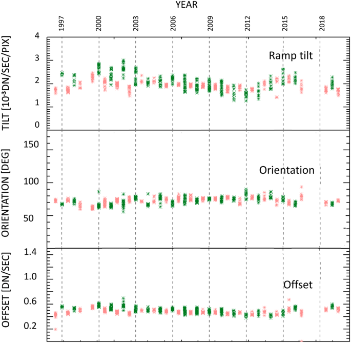

  

  Temporal variations of the ramp parameters of the unpolarized images: tilt, orientation, and offset. The colors distinguish the June ascending (pink) and December descending (green) nodes of the orbit of SOHO as it crosses the symmetry plane of the zodiacal cloud. At each node, several determinations of the parameters were obtained using different images.

• ii) A similar behavior is observed for the parameters of the ramps of the polarized images with, however, larger errors: typically 30%.

• iii) The geometry of the ramps of the polarized images is compatible with that of the unpolarized images.

These conclusions led us to adopt the ramp geometry of the unpolarized images for all polarized images with appropriate scaling of the parameters defined by the well-defined ratios of the individual polarized images to the unpolarized images.

References

Allen, C.W.: 1976, Astrophysical Quantities, 3rd edn., Astrophysical Quantities 1, Athlone, London. ADS.
Anderson, J.D., Krisher, T.P., Borutzki, S.E., Connally, M.J., Eshe, P.M., Hotz, H.B., Kinslow, S., Kursinski, E.R., Light, L.B., Matousek, S.E., Moyd, K.I., Roth, D.C., Sweetnam, D.N., Taylor, A.H., Tyler, G.L., Gresh, D.L., Rosen, P.A.: 1987, Radio range measurements of coronal electron densities at 13 and 3.6 centimeter wavelengths during the 1985 solar conjunction of Voyager 2. Astrophys. J. Lett. 323, L141. DOI. ADS.
Barlyaeva, T., Lamy, P., Llebaria, A.: 2015, Mid-term quasi-periodicities and solar cycle variation of the white-light corona from 18.5 years (1996.0-2014.5) of LASCO observations. Solar Phys. 290, 2117. DOI.
Bird, M.K., Volland, H., Paetzold, M., Edenhofer, P., Asmar, S.W., Brenkle, J.P.: 1994, The coronal electron density distribution determined from dual-frequency ranging measurements during the 1991 solar conjunction of the ULYSSES spacecraft. Astrophys. J. 426, 373. DOI. ADS.
Blackwell, D.E.: 1955, A study of the outer corona from a high altitude aircraft at the eclipse of 1954 June 30. I. Observational data. Mon. Not. Roy. Astron. Soc. 115, 629. DOI. ADS.
Blackwell, D.E., Petford, A.D.: 1966, Observations of the 1963 July 20 solar eclipse. ii, the electron density in the solar corona in the region 5 to 16 solar radii obtained from measurements of Fraunhofer line depth and the polarization of the f corona. Mon. Not. Roy. Astron. Soc. 131, 399. DOI. ADS.
Brueckner, G.E., Howard, R.A., Koomen, M.J., Korendyke, C.M., Michels, D.J., Moses, J.D., Socker, D.G., Dere, K.P., Lamy, P.L., Llebaria, A., Bout, M.V., Schwenn, R., Simnett, G.M., Bedford, D.K., Eyles, C.J.: 1995, The large angle spectroscopic coronagraph (LASCO). Solar Phys. 162, 357. DOI. ADS.
Cox, A.N.: 2015, Allen’s Astrophysical Quantities, fourth edn., Springer, New York.
Esposito, P.B., Edenhofer, P., Lueneburg, E.: 1980, Solar corona electron density distribution. J. Geophys. Res. 85, 3414. DOI. ADS.
Frazin, R.A., Vásquez, A.M., Thompson, W.T., Hewett, R.J., Lamy, P., Llebaria, A., Vourlidas, A., Burkepile, J.: 2012, Intercomparison of the LASCO-C2, SECCHI-COR1, SECCHI-COR2, and Mk4 coronagraphs. Solar Phys. 280, 273. DOI.
Hahn, J.M., Zook, H.A., Cooper, B., Sunkara, B.: 2002, Clementine observations of the zodiacal light and the dust content of the inner solar system. Icarus 158, 360. DOI. ADS.
Koomen, M.J., Detwiler, C.R., Brueckner, G.E., Cooper, H.W., Tousey, R.: 1975, White light coronagraph in OSO-7. Appl. Opt. 14, 743. DOI. ADS.
Koutchmy, S., Lamy, P.L.: 1985, The f-corona and the circum-solar dust evidences and properties. In: Giese, R.H., Lamy, P. (eds.), IAU Colloq. 85: Properties and Interactions of Interplanetary Dust, Astrophys. Space Sci. Lib. 119, Springer, Cham, 63. DOI. ADS.
Koutchmy, S., Picat, J.P., Dantel, M.: 1977, Etude polarimétrique de la couronne solaire observe a l’èclipse totale du 30 juin 1973 à l’aide d’un filtre neutre radial. Astron. Astrophys. 59, 349. ADS.
Krisher, T.P., Anderson, J.D., Morabito, D.D., Asmar, S.W., Borutzki, S.E., Delitsky, M.L., Densmore, A.C., Eshe, P.M., Lewis, G.D., Maurer, M.J., Roth, D.C., Son, Y.H., Spilker, T.R., Sweetnam, D.N., Taylor, A.H., Tyler, G.L., Gresh, D.L., Rosen, P.A.: 1991, Radio range measurements of coronal electron densities at 13 and 3.6 centimeter wavelengths during the 1988 solar conjunction of Voyager 2. Astrophys. J. Lett. 375, L57. DOI. ADS.
Lamy, P., Gilardy, H., Llebaria, A.: 2021, The F-corona from 24 years of LASCO observations. Solar Phys. (in preparation).
Lamy, P., Llebaria, A., Quémerais, E.: 2002, Solar cycle variation of the radiance and the global electron density of the solar corona. Adv. Space Res. 29, 373. DOI.
Lamy, P.L., Perrin, J.-M.: 1986, Volume scattering function and space distribution of the interplanetary dust cloud. Astron. Astrophys. 163, 269. ADS.
Lamy, P., Barlyaeva, T., Llebaria, A., Floyd, O.: 2014, Comparing the solar minima of cycles 22/23 and 23/24: the view from LASCO white light coronal images. J. Geophys. Res. Space Phys. 119, 47. DOI. ADS.
Lamy, P., Boclet, B., Wojak, J., Vibert, D.: 2017, Anomalous surge of the white-light corona at the onset of the declining phase of solar cycle 24. Solar Phys. 292, 60. DOI. ADS.
Lamy, P., Llebaria, A., Boclet, B., Gilardy, H., Burtin, M., Floyd, O.: 2020, Coronal photopolarimetry with the LASCO-C2 coronagraph over 24 years [1996 - 2019]. Solar Phys. 295, 89. DOI. ADS.
Leinert, C., Link, H., Pitz, E.: 1974, Rocket photometry of the inner zodiacal light. Astron. Astrophys. 30, 411. ADS.
Leinert, C., Pitz, E.: 1989, Zodiacal light observed by HELIOS throughout solar cycle No 21: stable dust and varying plasma. Astron. Astrophys. 210, 399. ADS.
Leinert, C., Link, H., Pitz, E., Giese, R.H.: 1976, Interpretation of a rocket photometry of the inner zodiacal light. Astron. Astrophys. 47, 221. ADS.
Leinert, C., Hanner, M., Richter, I., Pitz, E.: 1980, The plane of symmetry of interplanetary dust in the inner solar system. Astron. Astrophys. 82, 328. ADS.
Lemaire, J.F.: 2011, Determination of coronal temperatures from electron density profiles. arXiv. ADS.
Llebaria, A., Lamy, P., Bout, M.: 2004, Lessons learnt from the soho LASCO-C2 calibration. Proc. SPIE 5171, 27. DOI.
Llebaria, A., Thernisien, A.: 2001, Highly accurate photometric equalization of long sequences of coronal images. In: Starck, J-L., Mutragh, F.D. (eds.), Astronomical Data Analysis, Internat. Symp. Opt. Phot. CP-4477, SPIE, Bellingham, 265. DOI.
MacQueen, R.M., Csoeke-Poeckh, A., Hildner, E., House, L., Reynolds, R., Stanger, A., Tepoel, H., Wagner, W.: 1980, The High Altitude Observatory coronagraph/polarimeter on the Solar Maximum mission. Solar Phys. 65, 91. DOI. ADS.
Michard, R.: 1954, Densités électroniques dans la Couronne externe du 25 février 1952. Ann. Astrophys. 17, 429. ADS.
Michard, R.: 1956, Observations aériennes de la couronne externe à l’éclipse du 20 juin 1955. Ann. Astrophys. 19, 229. ADS.
Michard, R., Sotirovski, P.: 1965, Contributions à l’étude de la couronne lors de l’éclipse du 15 février 1961. ii. Photométrie et polarimètre de la couronne. Ann. Astrophys. 28, 96. ADS.
Michard, R., Dollfus, A., Pecker, J.C., Laffineur, M., D’Azambuja, M.: 1954, I Observations photométriques et polarimétriques de la Couronne externe. Ann. Astrophys. 17, 320. ADS.
Moran, T.G., Davila, J.M., Morrill, J.S., Wang, D., Howard, R.: 2006, Solar and heliospheric observatory/large angle spectrometric coronagraph polarimetric calibration. Solar Phys. 237, 211. DOI. ADS.
Morrill, J.S., Korendyke, C.M., Brueckner, G.E., Giovane, F., Howard, R.A., Koomen, M., Moses, D., Plunkett, S.P., Vourlidas, A., Esfandiari, E., Rich, N., Wang, D., Thernisien, A.F., Lamy, P., Llebaria, A., Biesecker, D., Michels, D., Gong, Q., Andrews, M.: 2006, Calibration of the SOHO/LASCO C3 white light coronagraph. Solar Phys. 233, 331. DOI. ADS.
Mueller, H.: 1948, The foundation of optics. J. Opt. Soc. Am. 38, 661.
Muhleman, D.O., Anderson, J.D.: 1981, Solar wind electron densities from Viking dual-frequency radio measurements. Astrophys. J. 247, 1093. DOI. ADS.
Mutschlecner, J.P., Keller, C.F., Tabor, J.E.: 1976, Electron density models of the solar corona. In: Bull. Am. Astron. Soc. 8, 397. ADS.
Newkirk, G. Jr.: 1967, Structure of the solar corona. Annu. Rev. Astron. Astrophys. 5, 213. DOI. ADS.
Pagot, E., Lamy, P., Llebaria, A., Boclet, B.: 2014, Automated processing of LASCO coronal images: spurious point-source-filtering and missing-blocks correction. Solar Phys. 289, 1433. DOI.
Pepin, T.J.: 1970, Observations of the brightness and polarization of the outer corona during the 1966 November 12 total eclipse of the Sun. Astrophys. J. 159, 1067. DOI. ADS.
Quémerais, E., Lamy, P.: 2002, Two-dimensional electron density in the solar corona from inversion of white light images-application to SOHO/LASCO-C2 observations. Astron. Astrophys. 393, 295. DOI.
Saito, K., Hata, S., Tojo, A.: 1972, Photometric and polarimetric analysis of the coronal streamers observed at the March 7, 1970 Mexican eclipse. Ann. Tokyo Astron. Obs. 13, 91. ADS.
Saito, K., Makita, M., Nishi, K., Hata, S.: 1970, A non-spherical axisymmetric model of the solar K corona of the minimum type. Ann. Tokyo Astron. Obs. 12, 51. ADS.
Stenborg, G., Howard, R.A., Stauffer, J.R.: 2018, Characterization of the white-light brightness of the f-corona between 5 and 24 elongation. Astrophys. J. 862, 168. DOI. ADS.
Thernisien, A., Morrill, J., Howard, R., Wang, D.: 2006, Photometric calibration of the LASCO-C3 coronagraph using stars. Solar Phys. 233, 155. DOI.
Wang, Y.-M., Sheeley, N.R. Jr.: 2003, On the fluctuating component of the Sun’s large-scale magnetic field. Astrophys. J. 590, 1111. DOI. ADS.
Acknowledgments
We thank our former colleagues at the Laboratoire d’Astrophysique de Marseille B. Boclet, M. Bout, and M. Burtin for their contributions to the early phases of this study. We are grateful to Y.-M. Wang for providing the Total Magnetic Field (TMF) data. The LASCO-C2 project at the Laboratoire d’Astrophysique de Marseille and the Laboratoire Atmosphères, Milieux et Observations Spatiales is funded by the Centre National d’Etudes Spatiales (CNES). LASCO was built by a consortium of the Naval Research Laboratory, USA, the Laboratoire d’Astrophysique de Marseille (formerly Laboratoire d’Astronomie Spatiale), France, the Max-Planck-Institut für Sonnensystemforschung (formerly Max Planck Institute für Aeronomie), Germany, and the School of Physics and Astronomy, University of Birmingham, UK. SOHO is a project of international cooperation between ESA and NASA.
Author information
Authors and Affiliations
Corresponding author
Ethics declarations
Disclosure of Potential Conflicts of Interest
The authors declare that they have no conflicts of interest.
Additional information
Publisher’s Note
Springer Nature remains neutral with regard to jurisdictional claims in published maps and institutional affiliations.