Anomalous Surge of the White-Light Corona at the Onset of the Declining Phase of Solar Cycle 24

Abstract

In late 2014, when the current Solar Cycle 24 entered its declining phase, the white-light corona as observed by the LASCO-C2 coronagraph underwent an unexpected surge that increased its global radiance by 60%, reaching a peak value comparable to the peak values of the more active Solar Cycle 23. A comparison of the temporal variation of the white-light corona with the variations of several indices and proxies of solar activity indicate that it best matches the variation of the total magnetic field. The daily variations point to a localized enhancement or bulge in the electron density that persisted for several months. Carrington maps of the radiance and of the HMI photospheric field allow connecting this bulge to the emergence of the large sunspot complex AR 12192 in October 2014, the largest since AR 6368 observed in November 1990. The resulting unusually high increase of the magnetic field and the distortion of the neutral sheet in a characteristic inverse S-shape caused the coronal plasma to be trapped along a similar pattern. A 3D reconstruction of the electron density based on time-dependent solar rotational tomography supplemented by 2D inversion of the coronal radiance confirms the morphology of the bulge and reveals that its level was well above the standard models of a corona of the maximum type, by typically a factor of 3. A rather satisfactory agreement is found with the results of the thermodynamic MHD model produced by Predictive Sciences, although discrepancies are noted. The specific configuration of the magnetic field that led to the coronal surge resulted from the interplay of various factors prevailing at the onset of the declining phase of the solar cycles, which was particularly efficient in the case of Solar Cycle 24.

1 Introduction

In a recent article, Barlyaeva, Lamy, and Llebaria (2015) have shown on the basis of 18.5 years (1996.0 – 2014.5) of observations with the LASCO-C2 coronagraph (Brueckner et al., 1995) onboard the Solar and Heliospheric Observatory (SOHO) that the global radiance of the K-corona closely tracks solar activity as recorded by standard indices and proxies. The maximum phase of the current Solar Cycle (hereafter abbreviated to SC) 24 has been remarkably quiet and weaker than the previous cycle, the yearly average of the sunspot number barely reaching 80, compared with a range of 106 to 190 in SC 23. Thus, it was quite surprising when the global radiance of the corona underwent a sudden increase starting in October 2014 that culminated in November – a rise by ${\approx}\,60\%$ that propelled the radiance to peak values comparable to those of the more active SC 23 – and finally leveled down to its pre-event value in April 2015.

The triggering event may have been the large sunspot complex AR 12192 first spotted on 17 October 2014, which turned out to be the largest ($\mbox{A} = 2740\times 10^{-6}$) since AR 6368 observed in November 1990 ($\mbox{A} = 3080\times 10^{-6}$). During the time AR 12192 was observable, it unleashed ten large solar flares, six of which were X-class types – including an X3.1 on 24 October 2014 – and four of which were of the M-class. This burst of activity in fact started in mid-2014 in a process that Sheeley and Wang (2015) called rejuvenation of the Sun’s large-scale magnetic field. According to these authors, several corroborating signs were observed, notably i) the amplitude of the Sun’s 27-day smoothed mean line of sight magnetic field derived from the Wilcox Solar Observatory (WSO)¹ measurements, which grew from 1.3 G in mid-2014 to reach a peak value of 2.5 G at the beginning of 2015, thus exceeding the peak values recorded during SC 23, and ii) the coronal inflows observed with LASCO occurring at unprecedentedly high rates and reaching the highest values measured since 1996 (Sheeley and Wang, 2014, 2015).

The purpose of the present article is to analyze in detail the simultaneous surge of the coronal radiance recorded by the LASCO-C2 white-light coronagraph. In Section 2 we describe the data used in this study and their reduction and introduce the solar indices and proxies used for comparison. Section 3 considers first the solar cycle variation of the radiance of the corona and then its variations on shorter timescales. Section 4 presents 2D reconstructions of the coronal electron density at the time of the maximum of the surge and 3D reconstructions based on time-dependent solar rotational tomography (SRT) over the whole considered period, which are compared to magnetohydrodynamic (MHD) models. Section 5 discusses our results in the framework of the unusual configuration of the solar magnetic field in late 2014, and we conclude in Section 6.

2 Observations and Data Reduction

LASCO-C2 is one of the two externally occulted coronagraphs of LASCO. It has been in continuous operation since January 1996, except for an interruption of a few months (from the end of June 1998 to March 1999) when the SOHO spacecraft lost its pointing. With its field of view extending from 2.2 to $6.5~\mathrm{R}_{\odot}$, it records the brightest part of the solar corona that is accessible to LASCO. Following the work of Lamy et al. (2014) and Barlyaeva, Lamy, and Llebaria (2015), the present analysis makes use of the routine polarization sequences since their temporal cadence (typically, one to four per day) is sufficient for our purpose and allows us to extract the K-corona following a classical procedure. A polarization sequence is composed of three linear polarized images of the corona obtained with three polarizers oriented at 60°, 0°, and −60° and an unpolarized image, all taken with the orange filter (bandpass of 540 – 640 nm) in the binned format of $512\times512$ pixels.

The standard preprocessing applied to the C2 raw, so-called “level 0.5”, images is continuously updated, in particular to reflect the temporal evolution of the performances of C2. This procedure as well as the separation of the K and F coronae and of the instrumental stray light are described in Lamy et al. (2014) and summarized in the appendix of Barlyaeva, Lamy, and Llebaria (2015). Several improvements have been introduced since the completion of these works; they marginally affected the integrated radiance, but were critical to the correct implementation of the time-dependent SRT (Section 4). Ultimately, we obtain a set of calibrated radiance ($B$) and polarized radiance ($pB$) maps of the K-corona that samples the period 1996 to the end of 2015 at the time of writing.

Following our aforementioned previous works, the radiance images of the K-corona are globally integrated in an annular region extending from 2.7 to $4.5~\mathrm{R}_{\odot}$, thus slightly restricting the field of view of C2 to avoid possible traces of stray light from the occulter in the inner region and dropping the outer region of low coronal signal. With respect to this last point, we note that the upper boundary is reduced to $4.5~\mathrm{R}_{\odot}$ compared with $5.5~\mathrm{R}_{\odot}$ used by Barlyaeva, Lamy, and Llebaria (2015) as a final choice for the LASCO products. Because the SOHO–Sun distance varies due to the slight eccentricity of the Earth orbit (and therefore of the L1 Lagrangian point), the size of the inner and outer radii expressed in pixels varies accordingly to precisely measure the same region of the solar corona throughout the year. The daily values of the integrated radiance are then averaged over each Carrington rotation (CR), whereas Barlyaeva, Lamy, and Llebaria (2015) used monthly averages. Finally, we do not consider the various sectors used by these authors (their Figure 1) since they are not relevant to the analysis of the surge of late 2014.

In order to place the variation of the radiance of the corona in the broader scope of solar activity and following our previous works, we consider several indices and proxies: sunspot number (SSN), sunspot area (SSA), total solar irradiance (TSI), total photospheric magnetic flux (TMF), and decimetric radio flux at 10.7 cm (F10.7). The SSN data come from WDC-SILSO data center,² the SSA data from the RGO/USAF/NOAA database,³ and the TSI data are from the newly scaled VIRGO composite.⁴ The total photospheric magnetic flux, calculated from the Wilcox Solar Observatory photospheric field maps, was kindly made available to us by Y.-M. Wang; details can be found in Wang and Sheeley (2003). The radio flux data come from the NOAA database.⁵

3 Temporal Variation of the Radiance of the Corona

We now analyze the temporal evolution of the global radiance of the K-corona as constructed in the above section and compare it with the evolutions of the selected indices and proxies. We first consider the whole time interval of 20 years – that is, the full SC 23 and a large part of SC 24 – covered by the LASCO observations. We then have a closer look at the four years extending over the maximum and early declining phases of SC 24, the latter having witnessed the surge of the coronal radiance. We finally analyze in detail the temporal evolution of the surge.

3.1 Solar Cycle Variation of the Radiance of the Corona

Figure 1 presents the long-term temporal evolution of the coronal radiance together with the evolutions of the selected proxies. The daily values are averaged over Carrington rotations, and the time interval extends over 20 years, from 1996.0 to 2015.9. In this set of graphs, the scales were chosen so that the curves closely match providing an easy comparison. It is important to realize, however, that the variations do not have the same amplitude. As has been found by Barlyaeva, Lamy, and Llebaria (2015), the coronal radiance tracks the solar (Schwabe) cycle well, as classically quantified by the sunspot number until mid-2014, with differences when compared to the different proxies, however. Its temporal evolution has been remarkably smooth during the ascending and maximum phases of SC24, especially when compared with SC 23, which was marked by several large-amplitude oscillations. A nearly constant value of ${\approx}\,1.6\times 10^{-10} B_{\odot}$ has prevailed since 2012, conspicuously lower than the peaks recorded in SC 23, which exceeded $2.5\times10^{-10}B_{\odot}$, in agreement with a weaker SC 24. An unexpected surge started in October 2014, culminated in November to a level comparable to the peaks of SC 23, and finally leveled down to its pre-event value in April 2015. It is remarkable that this surge took place at the onset of the declining phase of SC 24, as clearly indicated by the decrease of the sunspot number. In contrast, the sunspot area underwent a different evolution, the emergence of the extremely large AR 12192, which resulted in a peak in phase with that of the coronal radiance. The TSI and F10.7 proxies were not significantly affected by this activity surge, in contrast to the total magnetic field, whose variation by far best matches that of the radiance. This confirms one of the conclusions of Barlyaeva, Lamy, and Llebaria (2015), namely that the strongest correlation of the temporal variations of the coronal radiance – and consequently of the coronal electron density – is with the total magnetic flux, but it somewhat mitigates their other conclusion on the correlation with the total solar irradiance.

Figure 1

Temporal variation of the global radiance of the K-corona integrated from 2.7 to $4.5~\mathrm{R}_{\odot}$ compared with that of five proxies of solar activity from 1996.0 to 2015.9. From top to bottom: sunspot number, sunspot area, radio flux, total solar irradiance, and total magnetic field. All data are averaged over the Carrington rotation.

Figure 2 displays a zoomed version of the above figure limited to four years (2012.0 to 2015.9) and to SSN, SSA, and TMF. In the latter case, both the coronal radiance and TMF data have been normalized to their respective nearly constant values that they exhibited from January 2012 to September 2014. It is indeed quite remarkable that the four quantities, radiance, SSN, SSA, and TMF, have followed such a quasi-stable evolution during 2.75 years, albeit with larger fluctuations for SSA. These close-up views confirm the conclusions reached on the basis of Figure 1, but give a better insight into the surge. In addition to the total magnetic field, we introduce the open magnetic field as calculated by Sheeley and Wang (2015) and normalized as described above. As emphasized by these authors, “whereas the mean field reflects the variation of the non-axisymmetric components of the field, the amount of open flux depends on the entire field and therefore includes the contribution of the axi-symmetric component”. In addition to pre-event fluctuations about its mean value, which are more pronounced than for the TMF, the striking differences between the two variations are a much higher peak in late 2014 that reached a factor ${\approx}\,2.9$ compared to ${\approx}\,1.5$ for the TMF and a persistent high level thereafter, in contrast with both the radiance and TMF, which slowly returned to their respective pre-event values in the second half of 2015. Clearly, the correlation between radiance and TMF is overwhelming, implying that the variation of the radiance prominently reflects that of the non-axisymmetric components of the magnetic field.

Figure 2

Temporal variations of the global radiance of the K-corona integrated from 2.7 to $4.5~\mathrm{R}_{\odot}$ and of the sunspot number (upper panel), the sunspot area (middle panel), and the total and open magnetic fields (lower panel) from 1996.0 to 2015.9. In the lower panel, the radiance data and the total and open magnetic fields data are normalized to their respective pre-event values. All data are averaged over the Carrington rotation.

3.2 Short-Term Variations of the Radiance of the Corona

To further characterize the surge, we display in Figure 3 the daily evolutions of the coronal radiance and of the sunspot area from June 2014 to May 2015 (i.e. one year). We clearly see the emergence of the large sunspot complex (AR 12192) in mid-October 2014 and its periodic reappearance due to solar rotation (i.e. a period of ${\approx}\,27$ days). The radiance also undergoes periodic variations, but with a period of approximately half a solar rotation resulting from the alternative appearance of a local enhancement in the east and west hemispheres of the corona. This is illustrated by the synoptic map of the radiance displayed in Figure 4 that covers the time from June 2014 to May 2015. It has been constructed by extracting circular profiles at a radius of $3~\mathrm{R}_{\odot}$ from daily images of the coronal radiance and stacking them. It therefore simultaneously displays the east and west hemispheres of the corona and conspicuously confirms the alternative appearance of the enhancement on the east and west sides from October 2014 to February 2015. A close-up of this enhancement is offered by the Carrington map of the radiance at $3~\mathrm{R}_{\odot}$ (west limb) for CR2156 that is displayed in Figure 5 together with the synoptic chart of the HMI photospheric field.⁶ It is centered on an area close to the location of AR 12192 and has a remarkable inverse S-shape that extends from approximately longitude and latitude of 210° and 30° in the northern hemisphere to 320° and −60° in the southern hemisphere. This shape is consistent with the evolution of the non-axisymmetric component of the field and consequently of the shape of the magnetic “neutral line”, which progressively steepened as flux continued to emerge to become oriented along the south–north direction, as illustrated by Figure 4 of Sheeley and Wang (2015).

Figure 3

Daily variations of the global radiance of the K-corona integrated from 2.7 to $4.5~\mathrm{R}_{\odot}$ and of the sunspot area from June 2014 to May 2015.

Figure 4

Synoptic map of the radiance of the K-corona at $3~\mathrm{R}_{\odot}$ from June 2014 to May 2015. The color bar has units of $10^{-10}B_{\odot}$.

Figure 5

Carrington west-limb map of the radiance of the K-corona at $3~\mathrm{R}_{\odot}$ (upper panel) and synoptic chart of the HMI photospheric field for CR 2156 (lower panel). The color bars have units of $10^{-10}B_{\odot}$ for the radiance and gauss for the magnetic field.

4 Reconstructions in 2D and 3D of the Electron Density

We pursue our characterization of the surge by performing first a 2D reconstruction of the coronal electron density using the inversion method developed by Quémerais and Lamy (2002), restricted to the case of spherical symmetry and applied to a sequence of polarized radiance images obtained during the second half of November 2014 (CR 5927) when the enhancement was at its maximum (Figure 6). As expected for a corona of the maximum type, it is highly structured with a well-developed coronal hole in the south polar region, however. We concentrate our attention to the map of 24 November, when the central part of the local enhancement or bulge was approximately located in the plane of the sky on the west side and extract several radial profiles in the bulge and in the coronal hole to compare extreme cases (Figure 7). Each profile is averaged over a small sector of typically 10°. The comparison furthermore includes several classical models of the coronal electron density. For a corona of the maximum type (usually assumed to be spherical), we retain the following references: Allen (1973), Baumbach (1937), and van de Hulst (1950). For a corona of the minimum type, we retain the polar profiles of Allen (1973) and Saito et al. (1970). We also include the coronal hole model of Munro and Jackson (1977). We see that the profile along the bulge exceeds all classical maximum models by a factor of ${\approx}\,3$. The profile of the south polar hole is in remarkable agreement with the result of Munro and Jackson (1977), except for a slightly different gradient beyond $4.5~\mathrm{R}_{\odot}$.

Figure 6

Six maps of the coronal electron density obtained by 2D inversion of LASCO-C2 $pB$ images from 18 to 28 November 2014. The color bar is scaled to the logarithm of the electron density in units of $\mbox{cm}^{-3}$. The black disk corresponds to the occulter and the white circle to the Sun.

Figure 7

Radial profiles of the coronal electron density extracted from the maps displayed in Figure 6 on 22 November and from the 3D reconstruction for CR 2157. The profiles are centered on the bulge (top panel) and on the south coronal hole (bottom panel), respectively. Classical profiles as introduced in the text are overplotted for comparison: Allen (1973), Baumbach (1937), Munro and Jackson (1977), Saito et al. (1970), and van de Hulst (1950).

As a final effort to characterize the surge, we performed a 3D time-dependent reconstruction of the coronal electron density using the time-dependent solar rotation tomography (SRT) procedure recently developed by Vibert et al. (2016). It implements the multiple constraint regularization scheme, but limited to a spatio-temporal regularization in this present application. The relative weight of the two regularizations was tuned using a time-dependent MHD model of the corona based on observed magnetograms to build a time series of synthetic images of the corona.

Solving the inverse problem to reconstruct the coronal density requires building the projection matrix ($\mathbf{A}$), which is determined by the geometry and the physics of the problem. For each pixel located between $2.5~\mathrm{R}_{\odot}$ and $6.2~\mathrm{R}_{\odot}$, the geometry of the line of sight is specified using the information in the headers of the LASCO-C2 images and in the ancillary data, i.e. the date of observation, attitude and location of the SOHO satellite, and heliographic latitude, which is the tilt angle of the ecliptic with respect to the solar equatorial plane, also called the $B_{0}$ angle. The Thomson scattering function is determined for each line of sight and summed over four adjacent lines of sight. After building the matrix $\mathbf{A}$ for the LASCO images of size $512^{2}$ pixels, we resampled the images with a factor 2 to obtain images of size $256^{2}$ pixels that were used for the reconstruction. This increases the accuracy of the coefficients of the matrix. The inversion of the matrix $\mathbf{A}$ is performed in a spherical frame with a spatial resolution of 1° in both longitude and latitude and $0.1~\mathrm{R}_{\odot}$ in radial distance. The reconstruction requires that the corona be observed during at least half a solar rotation with a minimum cadence of about one image per day. We thus selected seven time intervals of 14 days that span seven Carrington rotations (CR2155 to CR2161) extending over six months, from 19 September 2014 to 16 March 2015, as specified in Table 1.

Table 1 Timelines of the seven 3D reconstructions of the coronal electron density.

Figure 8 displays six views of the 3D coronal electron density from six different vantage points for each of the seven selected time intervals; the same vantage points are used in the seven cases. The temporal evolution of the corona can be tracked by examining images along a column (same vantage point), whereas a row allows seeing a corona reconstructed in a given time interval from six different directions. A more spectacular view of the temporal evolution of the corona during the seven Carrington rotations (CR2155 to CR2161) is offered by a movie (see electronic supplementary material). The highly structured appearance of the corona is even more dramatically apparent in 3D views than in the 2D maps of Figure 6. The enhanced density in the bulge that created the radiance surge is prominently seen in the south hemisphere during four consecutive Carrington rotations, from 2156 to 2159, and tends to decrease and finally vanishes afterward. The color coding indicates that the electron density reaches peak values of ${\approx}\,1.6~10^{6}~\mbox{cm}^{-3}$ in the innermost part of the bulge. Average radial profiles of the electron density were constructed from the 3D cube by considering two different cones centered on the center of the Sun and probing different regions of the corona, by analogy to the sectors used in the case of the 2D maps. This allows averaging the density over increasing areas as it decreases with increasing heliocentric distance. The first cone probes the bulge; it is centered on a latitude and longitude of −40.5° and 283.5°, whereas the second cone probes the south coronal hole and is centered on a latitude and longitude of −40.5° and 73.5°; both cones have a full angular extent of 20° (Fig. 9).

Figure 8

Time-dependent SRT reconstructions of the coronal electron density for seven time intervals from CR 2155 (upper row) to CR 2161 (lower row). The corona is visualized from six different vantage points corresponding to the six columns. Following a column from top to bottom allows visualizing the temporal evolution of the corona from the same vantage point. Following a row from left to right allows visualizing a corona reconstructed in a given time interval from six different directions. The occulting disk has a radius of $2.5~\mathrm{R}_{\odot}$. The color bar is scaled to the logarithm of the electron density in units of $\mbox{cm}^{-3}$.

Figure 9

Two cones used to calculate the average radial profiles in the bulge and in the coronal hole.

Figure 7 compares the profiles obtained by 2D inversion and 3D time-dependent SRT reconstruction during the second half of November 2014 (CR 5927) when the enhancement was at its maximum. We note the perfect agreement of the profiles that are centered on the bulge. For the south polar hole, the 3D profile presents a better match to the model of Munro and Jackson (1977) than the 2D profile, to the point of being in perfect agreement except for a very slight deviation below $2.7~\mathrm{R}_{\odot}$.

The profiles for three consecutive Carrington rotations (CR 2156 to CR 2158) are displayed in Figure 10 together with the classical models introduced above, and the profiles are entirely consistent with the results obtained with the 2D inversion. The bulge reached its maximum radiance during CR 2157, during which it exceeded all classical maximum models by a factor of ${\approx}\,3$. The profiles of the south polar hole during CR 2156 and CR 2157 are in remarkable agreement with the result of Munro and Jackson (1977), whereas the profile of CR 2158 exhibits a slight excess.

Figure 10

Average radial profiles of the coronal electron density extracted from 3D cubes in two cones, one centered on the bulge (upper panel) and the other centered on the south coronal hole (lower panel). Classical profiles as introduced in the text and displayed in Figure 7 are overplotted for comparison.

Our 3D reconstruction of the electron density can be compared with the MHD calculations of Predictive Science Inc. available online:⁷ the two thermodynamic solutions labeled “std 101” and “std 201” and the polytropic “std 201” solution. The MHD calculations were performed for the six Carrington rotations considered above, CR 2155 to CR 2160, using HMI magnetograms as input, except for CR 2159, for which a GONG magnetogram was used because no HMI data are available. Comparing two data cubes is always challenging, and we present different visualizations of the resulting 3D electron densities. Figure 11 displays several 3D views produced from our tomographic reconstruction and the three MHD solutions for CR 2157. Figure 12 displays Mollweide equal-area projections of the electron density at $3.25~\mathrm{R}_{\odot}$ for six Carrington rotations from CR 2155 (top row) to CR 2160 (bottom row). Figure 13 displays radial profiles of the electron density calculated in two cones as defined above. Inspecting these figures leads to the following remarks.

• The two MHD thermodynamic solutions clearly outperform the polytropic solution both in the morphology of the corona and in the general level of the electron density, which is systematically too high in the latter solution. The lower panel of Figure 11 conspicuously shows coronal structures present in the latter solution that are absent both in our reconstruction and in the thermodynamic models, particularly in the north and southeast regions.

  Figure 11

  

  Comparison of the 3D reconstruction of the coronal electron density with different MHD models for CR 2157. The upper panel displays two views (one per row) from two different vantage points: the first column corresponds to the tomographic reconstruction, the second and third columns to the MHD thermodynamic std 101 and std 201 solutions. The lower panel displays a single view from the same vantage point as the second row of the upper panel. The left image represents the reconstructed electron density, and the middle and left images represent the MHD polytropic std 201 solution using two different color bars scaled to the logarithm of the electron density in units of $\mbox{cm}^{-3}$. The middle image uses the color bar of the upper panel. The left image uses the color bar below the lower panel. The occulting disk has a radius of $2.5~\mathrm{R}_{\odot}$.

  Figure 12

  

  Mollweide projections of the electron density at $3.25~\mathrm{R}_{\odot}$ for six Carrington rotations from CR 2155 (upper row) to CR 2160 (lower row). The first column corresponds to the tomographic reconstruction, the second and third columns to the MHD thermodynamic std 101 and std 201 solutions, respectively, and the fourth column to the MHD polytropic std 201 solution. The neutral lines of the MHD models are overplotted in black. The color bar is scaled to the logarithm of the electron density in units of $\mbox{cm}^{-3}$.

• The morphology of the corona produced by the two MHD thermodynamic models std 101 and std 201 are quite similar, as shown in Figure 11. However, careful inspection of the Mollweide projections reveals conspicuous differences prominently in the region of the bulge. They also differ in the general level of electron density, with std 101 producing higher densities.

• As also revealed by the Mollweide projections, the std 101 solution is in better agreement with our tomographic reconstruction than the std 201 solution, particularly in the region of the bulge, where the latter misses several coronal structures.

• The best agreement is obtained for CR 2157, which corresponds to the maximum of the surge, and to a lesser extent, for the two neighboring rotations, CR 2156 and CR 2158. Pronounced disagreements appear for the other Carrington rotations, notably the last two at longitudes ranging from 0° to 90°. This may result from the low resolution of the models on the website; the models are run automatically with a uniform distribution of points in longitude (J. Linker, private communication).

• The profiles of Figure 13 confirm that the generally higher level of the electron density of the thermodynamic std 101 is in better agreement with the our tomographic reconstruction than std 201. For the south coronal hole, our profile lies between the two MHD profiles, a quite remarkable result since these two profiles differ at most by ${\approx}\,50\%$ at $6~\mathrm{R}_{\odot}$. For the bulge, the std 101 profile is unable to reach our profile by a factor of ${\approx}\,2.2$ in the inner part of the corona, but is still closer than the std 201 profile, especially at large distances. The fact that the profile of the bulge produced by the polytropic std 201 model is slightly closer to the profile of our reconstruction than the thermodynamic std 101 solution is a direct consequence of the generally high level of the electron density in the former model, as is best seen in the case of the south coronal hole, where the excess reaches a factor of 20.

  Figure 13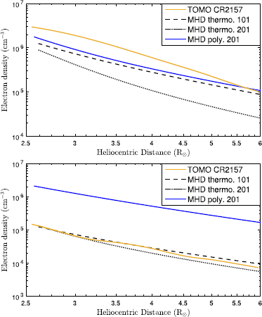

  

  Average radial profiles of the coronal electron density extracted from 3D cubes of the tomographic reconstruction, of the MHD thermodynamic std 101 and std 201 solutions, and of the MHD polytropic std 201 solution in two cones, one centered on the bulge (upper panel), and the other centered on the south coronal hole (lower panel).

On the basis of the perfect agreement that we obtain between the extreme profiles of the 2D inversion and the 3D reconstruction, we are inclined to think that the latter is fully correct and that the discrepancies with the thermodynamic std 101 and 201 profiles result from the difficulties and limitations intrinsic to the MHD thermodynamic models. However, the very fact that we obtain an agreement with the std 101 solution on a global scale and at finer scales in several cases as well as on the general level of electron density is extremely encouraging.

5 Discussion

The vigorous surge experienced by the white-light corona in late 2014 undoubtedly results from a local enhancement of the electron density associated with the emergence of AR 12192 that i) contributed to an unusually large increase of the magnetic field and ii) distorted the neutral sheet in a characteristic inverse S-shape. This resulted in the coronal plasma being trapped during several months in a similar pattern. In the view of Shibata, Ishii, and Kawamura (2015), the magnetic field became so strong that the reconnection point was very low (${<}\,6\times10^{4}~\mbox{km}$, the limit for eruption) so that flare ejecta were trapped and coronal mass ejections were prevented from erupting.

Sun et al. (2015) studied this active region in detail, particularly its magnetic configuration. They found that AR 12192 belongs to a class of confined active regions that produce non-eruptive flares as a result of weaker non-potentiality and stronger overlying field in the core region compared with unconfined ones. Sheeley and Wang (2015) presented an in-depth study of the behavior of the large-scale field and argued that its rejuvenation in late 2014 was not caused by a significant increase in the number of the sources of flux, but by the emergence of flux in a more efficient manner. Quantifying this effect, they found that AR 12192 accounted for only half of the increase in open flux, the other half came from the large unipolar region of positive polarity that was present just west of AR 12192. The authors concluded that the rejuvenation process depends upon the concomitance of three factors: i) the longitudinal phasing of the emerging sources, ii) the sizes of these sources, and iii) the contribution of the axisymmetric component of the field. They finally remarked that these three factors preferentially take place at the onset of the declining phase of a solar cycle since the newly reversed axisymmetric component helps to enhance the contribution of the equatorial component. Searching for similar occurrences during past cycles, the authors found maxima in the total and equatorial dipole fluxes during the past three solar cycles, in 1982 (SC 21), 1991 (SC 22), and 2003 (SC 23), see their Figure 6. Closer examination of the latter case reveals the presence of two peaks, one at the beginning of 2003 and the other in late 2003. Both peaks are present in the temporal variation of the radiance of the corona (Figure 1), but they do not stand out in the long-term evolution as the 2014 surge. Therefore, and while these pre-declining phase events certainly result from the interplay of various factors as proposed by Sheeley and Wang (2015), these two peaks optimally combined in late 2014 and were reinforced by the specific magnetic configuration of the confined AR 12192.

6 Conclusion

We have presented a detailed analysis and interpretation of the unexpected surge experienced by the white-light corona observed by the LASCO-C2 coronagraph in late 2014 as the current Solar Cycle 24 was initiating its declining phase. Its global radiance increased by 60%, reaching a peak value comparable to those of the more active Solar Cycle 23. Our main conclusions are summarized below.

• The relative temporal variation of the global radiance of the corona integrated in an annular region extending from 2.7 to $4.5~\mathrm{R}_{\odot}$ matches that of the total magnetic field remarkably well both in phase and in magnitude, unlike other indices and proxies of solar activity.

• The surge that appears during the second half of October 2014 and persisted until March 2015 underwent periodic variations with a period of approximately half a solar rotation. It resulted from a localized enhancement or bulge in the electron density with a characteristic inverse S-shape best seen on synoptic maps.

• This bulge is intimately connected to the emergence of the large sunspot complex AR 12192 in October 2014, the largest since AR 6368 observed in November 1990. The induced unusually large increase of the magnetic field and the distortion of the neutral sheet caused the coronal plasma to be trapped during several months along an inverse S-shape pattern.

• A 3D reconstruction of the electron density based on time-dependent solar rotational tomography confirms the morphology of the bulge. Together with 2D inversion of the coronal radiance, the reconstruction shows that the electron density level was well above the standard models of a corona of the maximum type, typically by a factor of 3. In addition, the reconstruction shows that its radial variation in the south coronal hole is remarkably consistent with the coronal hole model of Munro and Jackson (1977).

• A rather satisfactory agreement is found with the results of the std 101 polytropic MHD model produced by Predictive Science Inc., although discrepancies are noted.

• The specific configuration of the magnetic field that led to the spectacular coronal surge resulted from the interplay of various factors that usually prevail at the onset of the declining phase of the solar cycles. However, they optimally combined in late 2014 and were reinforced by the specific magnetic configuration of the confined AR 12192.

References

Allen, C.W.: 1973, Astrophysical Quantities, 3rd edn. University of London, The Athlon Press, London. ADS .
Barlyaeva, T., Lamy, P., Llebaria, A.: 2015, Mid-term quasi-periodicities and solar cycle variation of the white-light corona from 18.5 years (1996.0 – 2014.5) of LASCO observations. Solar Phys. 290, 2117. DOI .
Baumbach, S.: 1937, Strahlung, Ergiebigkeit und Elektronendichte der Sonnenkorona. Astron. Nachr. 263(6), 121. DOI .
Brueckner, G.E., Howard, R.A., Koomen, M.J., Korendyke, C.M., Michels, D.J., Moses, J.D., Socker, D.G., Dere, K.P., Lamy, P.L., Llebaria, A., Bout, M.V., Schwenn, R., Simnett, G.M., Bedford, D.K., Eyles, C.J.: 1995, The Large Angle Spectroscopic Coronagraph (LASCO). Solar Phys. 162, 357. DOI .
Lamy, P., Barlyaeva, T., Llebaria, A., Floyd, O.: 2014, Comparing the solar minima of cycles 22/23 and 23/24: The view from LASCO white-light coronal images. J. Geophys. Res. 119, 47. DOI .
Munro, R.H., Jackson, B.V.: 1977, Physical properties of a polar coronal hole from 2 to 5 solar radii. Astrophys. J. 213, 874. DOI .
Quémerais, E., Lamy, P.: 2002, Two-dimensional electron density in the solar corona from inversion of white light images application to SOHO/LASCO-C2 observations. Astron. Astrophys. 393, 295. DOI .
Saito, K., Makita, M., Nishi, K., Hata, S.: 1970, A non-spherical ax-symmetric model of the solar corona of minimum type. Ann. Tokyo Astron. Obs. 12, 53. ADS .
Sheeley, N.R. Jr., Wang, Y.M.: 2014, Coronal inflows during the interval 1996 – 2014. Astrophys. J. 797, 10. DOI .
Sheeley, N.R. Jr., Wang, Y.M.: 2015, The recent rejuvenation of the Sun’s large-scale magnetic field: A clue for understanding past and future sunspot cycles. Astrophys. J. 809, 113. DOI .
Shibata, K., Ishii, T., Kawamura, A.: 2015, Why big sunspot 12192 did not produce CME? In: Japan Geoscience Union Meeting, abstract number PEM07-32_E.
Sun, X., Bobra, M.G., Hoeksema, J.T., Liu, Y., Li, Y., Shen, C., Couvidat, S., Norton, A.A., Fisher, G.H.: 2015, Why is the great solar active region 12192 flare-rich but CME-poor? Astrophys. J. Lett. 804, L28. DOI .
van de Hulst, H.C.: 1950, The electron density of the solar corona. Bull. Astron. Inst. Neth. 11, 135. ADS .
Vibert, D., Peillon, C., Lamy, P., Frazin, R.A., Wojak, J.: 2016, Time-dependent tomographic reconstruction of the solar corona. Astron. Comput. 17, 144. DOI .
Wang, Y.M., Sheeley, N.R. Jr.: 2003, On the fluctuating component of the Sun’s large-scale magnetic field. Astrophys. J. 590, 1111. DOI .
Acknowledgements
We acknowledge fruitful discussions with N. R. Sheeley, Y.-M. Wang, and R. Howard (NRL). We are grateful to Y.-M. Wang for providing the total and open magnetic fields data. This study makes use of the MHD models of Predictive Science Inc., and we thank J. Linker for several clarifications. The LASCO-C2 project at the Laboratoire d’Astrophysique de Marseille is funded by the Centre National d’Etudes Spatiales (CNES). LASCO was built by a consortium of the Naval Research Laboratory, USA, the Laboratoire d’Astrophysique de Marseille (formerly Laboratoire d’Astronomie Spatiale), France, the Max-Planck-Institut für Sonnensystemforschung (formerly Max Planck Institute für Aeronomie), Germany, and the School of Physics and Astronomy, University of Birmingham, UK. SOHO is a project of international cooperation between ESA and NASA.
Author information
Authors and Affiliations
Corresponding author
Ethics declarations
Disclosure of Potential Conflicts of Interest
The authors declare that they have no conflicts of interest.
Electronic Supplementary Material
Below is the link to the electronic supplementary material.
Rights and permissions
About this article
Cite this article
Lamy, P., Boclet, B., Wojak, J. et al. Anomalous Surge of the White-Light Corona at the Onset of the Declining Phase of Solar Cycle 24. Sol Phys 292, 60 (2017). https://doi.org/10.1007/s11207-017-1089-0
Received:
Accepted:
Published:
DOI: https://doi.org/10.1007/s11207-017-1089-0