
Abstract
Delineation of management zones (MZs) are needed to manage fields in order to maximize economic return, minimize environmental impact, and improve soil and crop management. The MZs of uniform production potential may offer an effective solution to nutrient management. In this study, a total of 122 geo-referenced representative surface (0–250 mm depth) soil samples were collected from the study area covering an area of 6296 ha. Soil samples were analysed for pH, EC, CaCO3, organic carbon (SOC), available nitrogen (AN), available phosphorus (AP), available potassium (AK) and micronutrients (Fe, Mn, Zn and Cu). Their spatial variability was analyzed and spatial distribution maps were constructed using geostatistical techniques. Geostatistical analysis showed that exponential, rational quadratic, tetraspherical, pentaspherical and circular models were the best-fit models for soil properties and available nutrients. Further, geographical weighted principal component analysis (GWPCA) and possibilistic fuzzy C-means (PFCM) clustering algorithm were carried out to delineate the management zones based on optimum clusters identified using fuzzy performance index (FPI) and normalized classification entropy (NCE). The results revealed that the optimum number of MZs for this study area was four and there was heterogeneity in soil nutrients in four MZs. The study indicated that MZ-based soil test crop response recommendation reduces the application quantity of fertilizer significantly at a large extent. Therefore, the management zone concept can reduce agricultural inputs and environmental pollution, and maximize crop production.
Introduction
Hot arid environments pose many challenges for the management of agriculture. Soils of the arid tropics are highly variable. Variability in soil properties results mainly from the complex interactions between geology, topography, climate, as well as soil use (Jenny and Raychaudhuri 1960). The majority of arid ecosystems are characterized by erratic rainfall, in terms of both intensity and amount. Plant-nutrient balances are negative for many cropping systems. The long-term sustainability of many existing cropping systems in arid environments is questionable because of land degradation. Soils are usually poorly developed due to inherently low organic matter levels, and subject to degradation and structural decline. The fertilizer-use efficiency in crops of these regions is usually less than 25% and highly inconsistent (Singh et al. 2007). Crop responses to inputs such as fertilizers have generally been low and unprofitable to the farmer. Strategic application of fertilizers may improve use efficiency of the supplement with significant gains in both crop yield and biomass production. Ideally, application rates should be adjusted based on estimates of the requirements for optimum production at each location because there is always high spatial variability of nutrients within individual fields (Page et al. 2005; Ruffo et al. 2005). So, efficient techniques should be implemented to accurately measure within-field variations in soil properties and to delineate homogeneous management zones (MZs) for balanced application of fertilizers (Peralta and Costa 2013). The MZ concept advocates the identification of regions (management zones) within the area delimited by field boundaries. These subfield regions constitute areas of a field with similar characteristics, such as texture, topography and nutrient levels. However, it is difficult to accurately define management zones due to the complex interactions of all factors that could affect crop yield. Furthermore, the fact that factors interact in a dynamic way can make it very difficult to determine management by sub-fields.
Soil properties that limit crop yield within agricultural fields often vary considerably over space and time. Usually, this variability is intentionally ignored in soil sampling schemes, laboratory analyses and agronomic strategies for crop management. Hence, it appears that applying strategies for soil-specific conditions in the context of precision agriculture would have the potential to improve the way in which soils are currently managed. Quantification of the spatial variation of soil and terrain features has been facilitated by modern technologies that allow precise measurement. The advent of new spatially explicit technologies used in precision agriculture provides producers with the possibility of gathering information from small areas within the field and managing those areas differentially (Bullock et al. 2007). Mapping of soil nutrient levels would also facilitate proper monitoring and review of recommended farming technologies at locations from time to time. Use of geospatial tools and techniques in delineation of MZs assist in enhancing site-specific nutrient management in a sustainable manner. Moreover, knowledge about the soil fertility status may help to delineate correct MZs of particular regions for efficient nutrient management, crop production as well as environmental protection. Various traditional methods such as soil survey and topographical maps (Reyniers et al. 2006), crop yield-based management zone technique (Flowers et al. 2005; Hornung et al. 2006) and nutrient index technique (Jena et al. 2015) have been used for defining management zones.
In the last two decades, the application of geostatistical methods by soil scientists have been used to predict spatial variability of soil properties with different kriging methods over small to large spatial scale (Voltz and Webster 1990; Chatterjee et al. 2015). Geostatistics are used to detect, estimate and map the spatial patterns of regional variables. They are based on modelling and interpreting the semivariograms that relate any dissimilarity between paired data values to the distance between each sample pair (Goovaerts 1998). Several methods of cluster analysis such as c-means (Anderberg 1973) have been widely used to classify management areas. The application of fuzzy set theory (Burrough 1989) to clustering has enabled researchers to account for the continuous variation in natural soil variables (Guastaferro et al. 2010). The clustering procedure called fuzzy C-means (FCM), has been used to identify potential within-field management zones in precision agriculture (Peralta and Costa 2013). In the FCM algorithm, each data point has some degree of membership value which is used to determine the closeness of data points to a cluster (Bezdek 1981). FCM has a problem in that it creates noisy data points. To avoid this problem, Krishnapuram and Keller (1993) developed a new fuzzy cluster method named possibilistic c-means (PCM). PCM uses typicality values rather than membership value, but PCM has a problem with overlapping clusters. To avoid these problems, possibilistic fuzzy C-means (PFCM) is a better clustering algorithm as it has the potential to give more value to membership or typicality values (Pal et al. 2005). PFCM inherits both the properties of PCM and FCM that often avoids various problems like cluster coincidence and noisy sensitivity.
It is very difficult to separate the contribution of each soil property from soil fertility, making difficult the identification of the boundary between management zones. Thus, statistical methods such as principal components analysis (PCA) and clustering have been extensively used for delineation of MZs. However, the PCA method can be complemented using geographically weighted principal components analysis (GWPCA) when spatial heterogeneity occurs in the data (Harris et al. 2011). The use of GWPCA presents clear advantages over standard PCA since the former provides information regarding the spatial distribution of the percentage of variance and the variables with most influence in each of the components. In fact, a statistical hypothesis test is normally performed in GWPCA in order to establish the existence of spatial heterogeneity. Indeed, this method consists of performing a local PCA, based on neighbourhood of each data point, instead of a global PCA. The spatial principal components score obtained by GWPCA are used as input variables in the PFCM algorithm as a way to include autocorrelation in the clustering of spatial data. The hypothesis underlying the proposal is that application and incorporation of the GWPCA of soil variables into possibilistic fuzzy classification would produce MZs that avoid various problems like cluster coincidence and noisy sensitivity than those derived from the PCM and FCM algorithms. Therefore, greater separations of yield means among MZs are expected for the PFCM and GWPCA algorithm than for other implementations of PCA and FCM. The main goal of this study was to illustrate the proposed methodology, which accounts for spatial autocorrelation of soil variables, as a tool to identify MZs in precision agriculture.
Decisions regarding field management are usually undertaken based on the results of spatial variability of soil properties. Considering the high soil variability, it was hypothesized that soil properties that were studied in the same area differed in spatial distribution over time, which makes it more difficult to give proper recommendation for management practices based on the MZs. In view of the above facts, the present study was done to (i) characterize the spatial variability of the soil attributes affecting crop productivity using geostatistical analysis, (ii) identify management zones by using robust GWPCA and PFCM cluster algorithms, and (iii) evaluate the potential of defined management zones for site-specific nutrient management in the arid region of India.
Materials and methods
Study area
This study was conducted in Central State Farm, Suratgarh, located in the western plains of Rajasthan, India (29°20′53″–29°24′47″N, 73°30′00″–73°37′38″E) (Fig. 1). The total cultivated area of the farm is ~ 6296 ha which is intensively cultivated. The physiography of the study area is western plain-semi arid transitional plains which represent hot arid sandy plains and the Ghaggar flood plains agro-eco sub-region. The area has very scanty and erratic rainfall with extremely hot summers and cold winters. The average rainfall of the area is 286 mm. During the late 1960s, a canal network was brought in the northern part of the Thar Desert, Rajasthan, India which provides irrigation to the study area. The dominant soils are deep to very deep, either calcareous or non-calcareous and sandy in nature. Texture varied from sandy loam to clay loam with weak to moderate sub-angular blocky structure. It is a member of the fine-loamy mixed (cal.) hyperthermic, Typic Haplocambids (Soil Survey Staff 1999). Rice–wheat is the major annual crop rotation where rice is grown in kharif (rainy) and wheat during Rabi (winter) season. Rice is fertilized with mineral fertilizers at 150 kg N, 80 kg P2O5 and 60 kg K2O ha−1, while wheat is fertilized at 120 kg N, 60 kg P2O5 and 40 kg K2O ha−1. The N, P and K are supplied through urea, di-ammonium phosphate and muriate of potash, respectively. The rice–wheat system is adequately irrigated with ground and canal water.

Study site and soil-sampling points in irrigated hot arid environment of India
Soil sampling and analysis
One hundred twenty-two composite surface soil samples (0–250 mm) were collected from each grid point using 750 × 750 m grid map and handheld GNSS unit (GARMIN GPS Map 60-Garmin, USA) during 2015. The composite soil samples were collected in polythene bags and transported to the laboratory. Soil samples were then air-dried, thoroughly mixed, ground gently by a wooden mortar, and finally passed through a 2-mm sieve and stored in plastic bottles for soil analysis. Soil pH and electrical conductivity (EC) were measured as per the procedure described by Jackson (1973). Soil organic carbon (SOC) content of the soil samples was determined by the Walkley and Black (1934) method. Calcium carbonate (CaCO3) was analysed by rapid titration method (Richards 1954). Available N (AN) content was determined by alkaline permanganate method as described by Subbiah and Asija (1956). Available P (AP) was extracted with 0.5 M sodium bicarbonate (pH 8.5) as outlined by Olsen et al. (1954) and the P content in the extract was determined using ascorbic acid as reducing agent by a spectrophotometer. Available potassium (AK) was extracted with neutral 1N ammonium acetate (Hanway and Heidel 1952) and estimated by a flame photometer. The available micronutrients viz., Zn, Cu, Fe and Mn were extracted by diethylene tri-amine pentacetic acid (DTPA) as per the procedure developed by Lindsay and Norvell (1978).
Preliminary statistical analysis
Before conducting the GWPCA, an exploratory analysis of the data was carried out in order to find relationships between available nutrients and soil properties. The descriptive statistics like minimum, maximum, mean, median, standard deviation, coefficient of variation (CV), skewness, kurtosis and standard error (SE) were calculated for each soil property by using R-statistics software (R-Core-Team 2013). A correlation matrix was generated to compute the relationship among all the studied soil properties using Pearson’s correlation coefficient analysis.
Geostatistical analysis
To characterize the spatial distribution of soil attributes, semivariogram parameters were estimated using the geostatistical analyst of ArcGIS 10.3.1 software (Webster and Oliver 2007). Skewed soil properties were transformed using a natural logarithm to a nearly normal distribution before geostatistical analysis. The data were then back transformed using a weighted back transformation technique. In geostatistics, spatial variability of soil properties is expressed by semivariogram γ(h), which measures the average dissimilarity between the data separated by a vector h (Goovaerts 1998). It was computed as half of the average squared difference between the components of data pairs:
where, N(h) is the number of data pairs within a given class of distance and direction, z(xi) is the value of the variable at the location xi, z(xi+ h) is the value of the variable at a lag of h from the location xi. Experimental semivariograms \(\left[ {\hat{\gamma }\left( h \right)} \right]\) as obtained from the above equation were fitted with standard models using weighted least square technique and three standard spatial variations parameters were calculated: nugget (C0), sill (C + C0), and range (a). Weight was assigned as inversely proportional to the number of pairs for a particular lag. During semivariogram calculation, maximum lag distance was taken as half of the minimum extent of sampling area to minimize the border effect. In this study, omni-directional semivariogram was computed for each soil property because no significant directional trend was observed. Best-fit model with the lowest value of residual sum of square was selected for each soil property. Various semivariogram models such as circular, gaussian, exponential, tetraspherical, pentaspherical and rational quadratic were evaluated to determine the best-fit for explaining the spatial structure of each variable. The fitted models were then used in an ordinary kriging procedure to estimate different properties at non-measured points as interpolated values for mapping (Krige 1981).
Geographically weighted principal components analysis
Geographically weighted principal component analysis (GWPCA) is an extension of the global principal component analysis (PCA) to geographic data that aims to account for a certain spatial heterogeneity in the data (Harris et al. 2011). While global PCA analysis can provide information regarding global internal structure, it fails to consider spatial change in the covariance structure of the data. In GWPCA, the covariances are weighted as a function of the distance between the feature object and the features in the neighbourhood (Fotheringham et al. 2002). The GW covariance matrix is calculated as follows:
where X is the n × p matrix of data, being n the number of observations and p the number of covariates, and W (u,v) a n × n diagonal matrix of distance weights that depends on co-ordinates of location (u, v). Again the GWPCA defines the local eigen-structure at each spatial location (ui,vi) as follows:
where L(ui,vi) is a matrix of eigenvectors that represents the loadings of each variable on each principal component and V(ui,vi) the diagonal matrix of eigenvalues that represents the variances of the corresponding principal components. Similarly, component scores of the principal components are given by:
In general, two important decisions have to be considered before carrying out a statistical analysis: to transform or not the data, and how to deal with outliers. In PCA (and GWPCA), the most common pre-processing operations are logarithmic transformation and standardization. Standardization is required in PCA as well as in GWPCA because they are not scale invariant and to hold the normality assumption. In this case, the variable with the maximum standard deviation is AK (σ = 61.7), while the variable with the minimum standard deviation is SOC (σ = 0.17), so it is advisable to standardize the data to prevent the variables with larger variances dominating the first principal component.
Outliers are the extreme observations in a data, can artificially increase local variability and mask key features in local data structures, so a robust GWPCA (Harris et al. 2014) was performed instead of the basic approach. To perform a robust GWPCA, each local covariance matrix is estimated using the robust minimum covariance determinant (MCD) estimator. The MCD estimator searches for a subset of h data points that have the smallest determinant for their basic sample covariance matrix. The detail steps adopted for this robust GWPCA are as follow:
-
1.
Globally standardized the data and specify PCA with the covariance matrix. The same (globally) standardized data is also used in GWPCA calibrations, which are similarly specified with (local) covariance matrices (Harris et al. 2014).
-
2.
Components (say, k) having eigen value greater than one are retained assuming that PCs receiving high eigen values are best to represent soil properties and will be considered as a prior information to decide the number of components to be retained in GWPCA. (Schepers et al. 2004).
-
3.
Optimal bandwidth selection for the above retained components in GWPCA based on a minimum cross-validation score. Thus, for analysis, to generate a weighted matrix, an optimal adaptive bandwidth is found using a bi-square kernel function for robust GWPCA. The bi-square kernel function is given by:
$$w_{ij} \, = \,\left\{ {\begin{array}{*{20}c} {\left( {1 - \left( {\frac{{d_{ij} }}{b}} \right)^{2} } \right)^{2 } } & {if \left| {d_{ij} } \right| < b,} \\ 0 & {otherwise} \\ \end{array} } \right.$$(5)where the bandwidth is geographical distance b and \(d_{ij}\) is the distance between spatial locations of the ith and jth row in the data matrix.
-
4.
The standardized data are converted into a spatial data frame with incorporating the spatial data points and run the robust GWPCA using GW model R package (Gollini et al. 2015). To remove effect of outliers, the MCD estimator searches for a subset of h = 0.75 data points has been considered in this study
-
5.
Compute the GWPCA score for each covariate at each data point using the GWPCA components and the data matrix, which will be the input for the PFCM algorithm. Figure 2 is a schematic representation of the proposed methodology.
Fig. 2 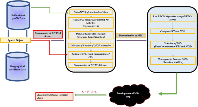
Schematic representation of the proposed methodology

Possibilistic fuzzy C-means algorithm
The possibilistic fuzzy C-means (PFCM) was used to divide the field into different unique management zones. The PFCM statistically minimizes the within-group variability while maximizing the among-group variability to produce homogeneous groups. The PFCM is a mixed clustering algorithm, which overcomes the noise sensitivity problem of FCM, and tries to eliminate the coincident clusters problem of PCM. It also provides a more informative description of the data than FCM and PCM, since it provides both membership and typicality information simultaneously. The purpose of this algorithm is to minimize the following objective function:
Subject to the constraint \(\mathop \sum \limits_{i = 1}^{c} \mu_{ik} = 1 \forall k\), and \(\mu_{ik} \ge 0,t_{ik} \le 1\). Here b > 0, a > 0, η > 1, m > 1 and \(\gamma_{i } > 0\) used as user defined constants. Constants a, b is used to define the relative proportion of typicality and membership values. Here, \(U = \left[ {\mu_{ik} } \right]\) is a membership matrix similar as in FCM and,\(T = \left[ {t_{ik} } \right]\) a typicality matrix similar as in PCM algorithm. Let Z is a dataset, \(Z_{k} = \left\{ {z_{1} ,z_{2 } , \ldots ,z_{n} } \right\}\) and list of clusters centres represented by \(V_{i} = \left\{ {v_{1} ,v_{2 } , \ldots ,v_{c} } \right\}\). Algorithmic steps for possibilistic fuzzy c-means (PFCM):
-
1.
Initialize the number of clusters i.e. c. In this study, a minimum of two clusters and maximum of eight clusters were set as initial parameters.
-
2.
Randomly set the clusters centroids. In this analysis, a minimum of two centroids to a maximum of eight centroids were considered.
-
3.
The FCM Algorithm was run and the membership values of each data point for different clusters were computed by minimizing the following objective function.
$$\mathop {\hbox{min} }\limits_{{\left( {Z,U,V} \right)}} \left\{ {J\left( {Z,U,V} \right) = \mathop \sum \limits_{i = 1}^{C} \mathop \sum \limits_{k = 1}^{n} \mu_{ik}^{m } \left\| {Z_{k} - V_{i}^{2} } \right\| } \right\}$$(7) -
4.
With the help of these results, the penalty parameter \(\gamma_{i }\) was calculated for every cluster using Eq. 8.
$$\gamma_{i } = K\frac{{\mathop \sum \nolimits_{k = 1}^{n} \mu_{ik}^{m } \left\| {Z_{k} - V_{i}^{2} } \right\| }}{{\mathop \sum \nolimits_{k = 1}^{n} \mu_{ik}^{m } }}$$(8) -
5.
Calculated the membership values \(U = \left[ {\mu_{ik} } \right]\) when distance between data point and centroid was greater than 0.
$$\mu _{{ik}} = \frac{1}{{\sum\nolimits_{{j = 1}}^{c} {\left( {\frac{{\left\| {Z_{k} - V_{i} } \right\|}}{{\left\| {Z_{k} - V_{j} } \right\|}}} \right)^{{\frac{2}{{m - 1}}}} } }}$$(9) -
6.
Calculated the typicality values \(T = \left[ {t_{ik} } \right]\) when distance between data point and centroid was greater than 0.
$$t_{ik} = \frac{1}{{1 + \left( {\frac{b }{\eta }\left\|Z_{k} - V_{i}^{2}\right\|} \right)^{{\frac{1}{{\left( {\eta - 1} \right)}}}} }}$$(10) -
7.
Calculated the center Vector i using:
$$v_{i } = \frac{{\mathop \sum \nolimits_{k = 1}^{n} \left( {a\mu_{ik}^{m } + bt_{ik}^{\eta } } \right) Z^{k } }}{{\mathop \sum \nolimits_{k = 1}^{n} \left( {a\mu_{ik}^{m } + bt_{ik}^{\eta } } \right) }}$$(11) -
8.
Stopped when the error is less or equal to \(\left\| {V_{{k + 1}} - V_{k} } \right\|{\text{ < }}\;\delta\), otherwise moved to step 6.
In this study, the PFCM was performed using the “ppclust” R-package (Cebeci et al. 2018). Settings used in R software were as follows: a = 2; b = 3; η = 2; fuzziness exponent (m) = 1.5; the stopping criterion (δ) = 0.0001; minimum number of zones = 2; maximum number of zones = 8. Two cluster validity functions; including fuzzy performance index (FPI) (McBratney and Moore 1985) and normalized classification entropy (NCE) were used as indicators of optimum cluster number (Bezdek 1981) as follows:
where c is the number of clusters and n is the number of observations, μik is the fuzzy membership and loga is the natural logarithm. The FPI measures the degree of fuzziness created by a specified number of classes. Values of FPI may range from 0 to 1. Values approaching 0 indicate distinct classes with little membership sharing while values near 1 indicate no distinct classes with a large degree of membership sharing. The NCE is an estimate of the amount of disorganization created by a specified number of classes. The optimal number of clusters for each computed index (FPI and NCE) is obtained when the index is at the minimum, representing the least membership sharing (FPI) and greatest amount of organization (NCE) as a result of the clustering process (Fridgen et al. 2004). Furthermore, analysis of variance was used to indicate heterogeneity among different MZs. Descriptive statistics were obtained by R software. ArcGIS 10.3.1 software (ESRI, Redlands, California) was used for geostatistics analysis and mapping. R software was used in implementing the GWPCA and PFCM clustering algorithm.
Results and discussion
Descriptive statistics of soil properties
Descriptive statistics of the soil variables are reported in Table 1. It was evident that this site is slightly to strongly alkaline, with a pH ranging from 7.28 to 9.70 having the lowest coefficient of variation (CV). Other researchers also documented a smaller variation of soil pH compared to other soil properties (Reza et al. 2017; Shukla et al. 2017). Low variability of pH may be attributed to the fact that pH values are log scale of proton concentration in soil solution; there would be much greater variability if soil reaction is expressed in terms of proton concentration directly. Generally, soil buffering capacity resists the abrupt change of soil pH or its high variability under different cropping systems and its management in the study area. The rest of the soil properties exhibited moderate (CV 25–75%) variability except EC. In comparison with other properties, EC had the highest CV (92.8%) with values ranging from 0.10 to 1.99 dS m−1. This is mainly because application of saline groundwater as irrigation source, resulting in marked changes in EC over small distances. The SOC content in the study site varied from 0.10 to 0.97% and meets the need for rice and wheat growth with a mean of 0.44%. According to Moharana et al. (2017), SOC content in this area was adequate for a rice–wheat cropping system. Available K content was high, similar findings also reported by Singh et al. (2007). The available P content was high, with a mean of 31.3 kg ha−1, which was due to formation of insoluble Ca–P complexes in an arid environment. The mean values of Zn, Cu, Fe and Mn in this region were 0.61, 1.46, 14.2 and 7.93 mg kg−1, respectively and concentration of these micronutrients varied widely. This variation of soil properties in the studied areas may be due to adoption of different soil management practices including variation in fertilizer application and other crop management practices (Srinivasarao et al. 2014; Shukla et al. 2017). Overall, the soil in the study area was characterized by medium nutrient levels and high variability. The uniform application of nutrients resulted in varying supply of nutrients with respect to their content in the specific location of the studied area, which caused spatial variability in crop yield.
The Pearson linear correlation analysis results (Table 2) showed that soil pH was significantly negatively correlated to SOC (r = − 0.33, P < 0.01), CaCO3 (r = 0.44, P < 0.01), AN (r = − 0.29, P < 0.01) and AP (r = − 0.27, P < 0.01), indicating that increasing pH might significantly decrease the level of available N in this area. Singh et al. (2007) and Moharana et al. (2017) found similar results in hot arid environments. SOC showed a significantly positive correlation with available macronutrients (N, P and K), and negatively correlated with CaCO3. The significant correlation between the selected soil properties indicated that PCA should be performed to summarize the principal sources of variability in the data.
Geostatistical analysis
In order to identify the possible spatial structure of different soil properties, semivariograms were calculated and the best models that describe these spatial structures were identified. The experimental semivariogram of the soil properties were fitted with theoretical models (Fig. 3) and the results are presented in Table 3. Root-mean-squared residuals were found minimally corresponding to the pentaspherical model for pH, SOC and available Zn contents and therefore are considered the best-fit model for these soil parameters. The J Bessel, rational quadratic, teraspherical, exponential and circular models were found best for the CaCO3, AP, AK, Mn and Cu, respectively. Similarly, a Gaussian model was found best for the AN and Fe. Spatial structural parameters, i.e., nugget, sill and range corresponding to the best-fit model are also given in Table 3. All soil properties showed positive nugget, which can be explained by sampling error, short range variability, random and inherent variability. The relative proportion (i.e. nugget/sill) of < 25%, 25–75%, and > 75% could be used to describe the degree of the spatial structure that showed strong, moderate and weak spatial autocorrelation, respectively. Usually, strong, moderate and weak spatial dependence of soil properties can be attributed to intrinsic factors of soil properties and mineralogy, extrinsic factors such as anthropogenic activities, and both intrinsic and extrinsic factors respectively (Cambardella et al. 1994; Liu et al. 2006). In the present study, AK showed a strong spatial dependence whereas soil pH, AN, Zn and Cu showed a moderate spatial dependence. The other parameters like EC, SOC, CaCO3, AP, Fe and Mn showed weak spatial dependence. This variation of soil nutrients might be attributed to the improper doses of fertilizer application in crops by the farmers of the study area. The ‘range’ of the semivariogram was the distance (h) at which semi-variance attained the maximum value (sill), and the sill approximately equalled the sample variance (Reza et al. 2017). The range expressed as distance could be interpreted as the diameter of the zone of influence that represented the average maximum distance over which a soil property of two samples was related. The measured soil attribute of two sampling points became similar with decreasing distance between these locations within its spatial range. The range of spatial variation was found ~ 1000 m for pH and SOC content. This indicated that, in the field, these soil parameters were spatially correlated with each other up to a distance of 1000 m, beyond which the variation was considered as random. The range for AP was 1790 m, which was higher than the remaining soil nutrient contents. Spatial correlation structure for available Fe and Zn were comparatively better than those for Mn and Cu.

Best-fitted semivariogram models for selected soil properties. a pH, b EC, c SOC, d CaCO3, e available N, f available P, g available K, h available Cu, i available Zn, j available Mn and k available Fe
Spatial distribution maps for all soil properties are shown in Fig. 4. All soil nutrients showed high levels in the northeast and north, and low levels in the south and southwest direction, which was mainly caused by heterogeneous management and fertilizer application. SOC and AN showed similar spatial variability, high values occurred in the northeast area and low values in the southwest. The distribution maps for AN, AP, AK and micronutrients were very similar, decreasing from northeast to southwest direction. This was probably due to parent material, irrigation, fertilizer application and crop planting. Soil pH, EC and CaCO3 displayed similar patterns, with high values in the west and south and low values in the east. The quantitative information obtained from these maps could be used to facilitate site-specific management and apply variable rate technology for best management. The distribution maps could be used to design site-specific management strategies to increase crop yields while minimizing environmental pollution and input costs.

Spatial distribution map of soil properties and available nutrients in irrigated hot arid environment of India. a pH, b EC, c CaCO3, d SOC, e available N, f available P, g available K, h available Zn, i available Cu, j available Fe and k available Mn. Values in parenthesis in legends represent the % area for that particular legend class
Global principal components analysis
To understand any geographically weighted model output, it is always important to fit the usual global model for context excluding the spatial effect. In this respect, a PCA was conducted on the eleven variables describing soil properties and fertility. Table 4 shows that the first four PCs have eigenvalues greater than unity, and for these four PCs, the cumulative percentage of total variance (PTV) exceeds 66%. The four PCs (PC1, PC2, PC3 and PC4) explained 28, 17, 12 and 9% of total variance, respectively. The SOC, AN and AP had the most significant influence on PC1. For PC2, Zn and Cu produced a large contribution relative to the other variables. The PC3 was dominated by Mn. Similarly, EC and CaCO3 had the most significant influence on PC4. All these properties are probably related to soil fertility, but the absence of spatial information in PCA, does not allow confirmation of this hypothesis. Consequently, the scores map of PC1 was very similar to the distribution maps for pH, SOC, AN and AP. In the same way, the scores map of PC2 was very similar to the map of AK, Zn and Cu, and the distribution maps of PC3 and EC were similar. The most obvious spatial concentrations of large negative scores are in the north-eastern part of the farm, and large positive scores are in the eastern part (Fig. 5), although, there is no clear geographical trend. The map suggests marked spatial variation in soil characteristics, but it is not possible to assess which variables explain most variation in particular regions. GWPCA provides additional information which is obscured by PCA, and the former comprises the major focus in this paper.

PC scores maps for GPCA and GWPCA. GPCA global principal component analysis, GWPCA geographically weighted principal component analysis, PC principal component
Geographically weighted principal components analysis
The GWPCA is now applied to account for expected spatial heterogeneity in the soil fertility. The GWPCA results are compared with those from global PCA throughout. To compare GWPCA and PCA, only the first four components (PC1 to PC4) from each calibration are considered. PCs scores from GWPCA and the global PCA are mapped in Fig. 5. Observe that for GWPCA, a full n = 122 valued scores data set is available at each location for each component. Thus, the GWPCA scores data that are mapped are only those that fully correspond to their location. For each location, a matrix of four principal components was obtained as well as the corresponding proportion of variance explained by them and the winning variables (those with the highest loadings). The optimal bandwidth of n = 69 has been obtained from the bi-square kernel function for k = 4 components considering a minimum cross-validation score. To provide a robust GWPCA, the MCD estimator was specified for a subset of h = 0.75n (n = 122) data points that has the smallest determinant for their basic sample covariance matrix according to the recommendation of Varmuza and Filzmoser (2009). The majority of the soil samples account for between 85.9 and 93.8% of the variance in the data with an average of 89.9%, which explains 23% more variability than Global PCA. This percentage variance is greater in the center and eastern area of the region as well as at the western edge of the region. In each location, the variable with the highest loading (in absolute value), the so-called winning variable, in each GWPC was determined. The winning variables are different depending on the location.
Clustering analysis for delineating management zones
Geographically weighted principal components score for the first four PCs were imported into “ppclust” package of R software for management zone analysis. The PFCM cluster algorithm was performed to classify the four PCs into MZs and the detail of setting for this analysis has been explained in the material and methodology section. PFCM algorithm repeated multiple times to get cluster validity indices for 2 to 8 MZs. The values of cluster validity indices FPI and NCE are plotted against the number of classes in Fig. 6. The optimum number of clusters is determined when each index is at the minimum representing the least membership sharing (FPI) or greatest amount of organization (NCE) as a result of the clustering process. It was observed that the FPI and NCE values were minimum for four clusters and the membership for all observations in different clusters were calculated. Management zones map was developed by performing zonal statistics in ArcGIS 10.3.1 (Fig. 7). For characterizing the spatial variability of soil properties and availability of nutrients for delineating MZs, Tukey multiple comparisons test was performed to assess the effectiveness of using combination of GWPCA and fuzzy cluster algorithm. This analysis indicated that the four MZs created were distinctly different from each other as also observed by other researchers (Xin-Zhang et al. 2009; Davatgar et al. 2012; Tripathi et al. 2015). In addition, the analysis of variance indicated that significant statistical difference (P < 0.01) existed among the four MZs for all properties (Table 5).

Fuzzy performance index (FPI) and normalized classification entropy (NCE) calculated for identifying the optimum clusters for the study area

Management zone map for four clusters in irrigated hot arid environment of India
Heterogeneity of soil chemical properties among different MZs was evident from the analysis (Table 5). The average values for EC, CaCO3, AN, AK, Cu, Zn, Mn and Fe within each management zone were significantly different at P < 0.01. There was no significant difference for pH, SOC and AP among the MZs. MZ 4 is covering the major portion of the study area (41.5%) followed by MZ 3(31.3%), MZ2 (18.1%) and MZ1 (9.1%). The difference in soil properties in four MZs may be due to crop and management practices, soil types and agro-ecological factors (Ortega and Santibanez 2007; Shukla et al. 2017). This zonation concept will be helpful in effective and efficient scientific management of nutrients. Geostatistical analysis demonstrated the spatial heterogeneity of soil properties, particularly macro and micronutrients in the study region. Hence, the information regarding MZs could be used by farmers and other stakeholders for site specific nutrient management.
Fertilizer recommendation strategies
The present status of spatial variations in the available nutrient (NPK) contents of the soils in the given study brings out the potential of site-specific fertilizer management strategies for applying the exact requirement of nutrients to individual fields and crops within a domain of individual holdings, supported by a range of management practices. The small-scale production systems in India are characterized by a very large number of land holdings and therefore, the implementation of field-specific fertilizer application schedule would be a rather difficult proposition unless one is able to group the fields with similar indigenous nutrient supplying capacity as unique management zones and treat them as one entity. The soil test crop response (STCR) equations, developed by the All India Coordinated Research Project (AICRP), Indian Council of Agricultural Research (ICAR), which are unique for each crop, soil type and climatic conditions, are used in described management zones for production of rice and wheat. The established STCR equation for, rice in the present study area is FN = 3.60T–0.253N, FP2O5 = 2.29T–0.82SP, FK2O = 2.61T–0.19SK and for wheat, the equation is FN = 7.87T–0.76SN, FP2O5 = 3.04T–1.50SP, FK2O = 4.07T–0.26 SK, where FN, FP2O5, and FK2O are the fertilizer requirement to obtain the target yield of 5 t/ha in case of rice and wheat, and SN, SP, and SK are the soil test values for N, P, and K. Indeed one may interlink these equations with MZs map by putting the calculated soil test values in the equations for determining the fertilizer rates. The amount of fertilizer savings in rice–wheat production system for the four MZs was calculated (Table 6). This study indicated that, under similar agro-climatic conditions and management practices, site-specific nutrient management reduces the application quantity of fertilizer significantly at a large extent. Therefore, the management zone concept can reduce the agricultural inputs and environmental pollution, and increase farmer incomes. Cluster analysis will reduce within-zone variability by grouping data points into naturally occurring clusters, and provides some information for site-specific fertilization with the aim of maximizing crop production across the entire zone.
Conclusion
Research in site-specific fertilization has focused on dividing a field into a few relatively uniform homogeneous zones as a practical, environmentally sustainable and cost-effective approach for managing soil variability. In this study, the spatial variability of eleven soil properties was quantified using geostatistical methods and was aggregated into MZs using GWPCA and fuzzy clustering algorithms. Geostatistical analysis revealed that circular, exponential, tetraspherical, pentaspherical and rational quadratic models were best fit models for estimated soil parameters. Soil properties and available nutrients showed spatial heterogeneity with weak to moderate spatial dependence. Results indicated that the optimal number of MZs was four. The analysis indicated heterogeneity in soil properties among the four MZs. The MZ-based soil test crop response recommendation reduces the application quantity of fertilizer significantly at a large extent. The prescribed fertilizer doses based on MZ maps could be the primary guide for farmers to adopt site-specific nutrient management, which satisfies the criteria of management zones to be simple, functional, easy to understand and economically feasible. Therefore, the MZs take into account completeness and continuity, and facilitate farming operations. At the same time, use of MZs saves fertilizer. These results provide information for rationally managing soil fertilizer site-specifically while minimizing detrimental environmental impacts and improving overall productivity.
References
Anderberg, M. R. (1973). Cluster analysis for applications. New York, USA: Academic Press Inc.
Bezdek, J. C. (1981). Pattern recognition with fuzzy objective function algorithms. New York, USA: Plenum.
Bullock, D. S., Kitchen, N., & Bullock, D. G. (2007). Multidisciplinary teams: A necessity for research in precision agriculture systems. Crop Science,47, 1765–1769.
Burrough, P. A. (1989). Fuzzy mathematical methods for soil survey and land evaluation. Journal of Soil Science,40, 477–492.
Cambardella, C. A., Moorman, T. B., Novak, J. M., Parkin, T. B., Karlen, D. L., Turco, R. F., et al. (1994). Field-scale variability of soil properties in central Iowa soils. Soil Science Society of America Journal,58, 1501–1511.
Cebeci, Z., Yildiz, F., Kavlak, A. T., Cebeci, C., & Onder, H. (2018). ppclust: Probabilistic and Possibilistic Cluster Analysis. R package version 0.1.1, URL https://CRAN.R-project.org/package=ppclust. Accessed 22 August 2018.
Chatterjee, S., Santra, P., Majumdar, K., Ghosh, D., Das, I., & Sanyal, S. K. (2015). Geostatistical approach for management of soil nutrients with special emphasis on different forms of potassium considering their spatial variation in intensive cropping system of West Bengal. India. Environmental Monitoring and Assessment,187, 183. https://doi.org/10.1007/s10661-015-4414-9.
Davatgar, N., Neishabouri, M. R., & Sepaskhah, A. R. (2012). Delineation of site specific nutrient management zones for a paddy cultivated area based on soil fertility using fuzzy clustering. Geoderma,173–174, 111–118. https://doi.org/10.1016/j.geoderma.2011.12.005.
Flowers, M., Weisz, R., & White, J. G. (2005). Yeild-based management zones and grid sampling strategies: Describing soil test and nutrient availability. Agronomy Journal,97(3), 968–982.
Fotheringham, A. S., Brunsdon, C., & Charlton, M. (2002). Geographically weighted regression: The analysis of spatially varying relationships. Chichester, UK: Wiley.
Fridgen, J. J., Kitchen, N. R., Sudduth, K. A., Drummond, S. T., Wiebold, W. J., & Fraisse, C. W. (2004). Mnagement zone analyst (MZA): Software for subfield management zone delineation. Agronomy Journal,96, 100–108.
Gollini, I., Lu, B., Charlton, M., Brunsdon, C., & Harris, P. (2015). GWmodel: An R package for exploring spatial heterogeneity using geographically weighted models. Journal of Statistical Software,63, 1–50.
Goovaerts, P. (1998). Geostatistical tools for characterizing the spatial variability of microbiological and physico-chemical soil properties. Biology and Fertility of Soils,27, 315–334.
Guastaferro, F., Castrignanò, A., Benedetto, D., Sollitto, D., Troccoli, A., & Cafarelli, B. (2010). A comparison of different algorithms for the delineation of management zones. Precision Agriculture,11, 600–620.
Hanway, J. J., & Heidel, H. (1952). Soil analysis methods as used in Iowa State College Soil Testing Laboratory. Iowa Agriculture,57, 1–31.
Harris, P., Brunsdon, C., & Charlton, M. (2011). Geographically weighted principal components analysis. International Journal of Geographical Information Science,25, 1717–1736.
Harris, P., Brunsdon, C., Charlton, M., Juggins, S., & Clarke, A. (2014). Multivariate spatial outlier detection using robust geographically weighted methods. Mathematical Geosciences,46, 1–31.
Hornung, A., Khosla, R., Reich, R., Inman, D., & Westfall, D. G. (2006). Comparsion of site specific management zones: Soil-color-based and yield-based. Agronomy Journal,98(2), 407–415.
Jackson, M. L. (1973). Soil chemical analysis. New Delhi: Prentice Hall of India Pvt. Ltd.
Jena, R. K., Duraisami, V. P., Sivasamy, R., Shanmugasundaram, R., Krishnan, R., Padua, S., et al. (2015). Spatial variability of soil fertility parameters in Jirang Block of Ri-Bhoi District, Meghalaya. Clay Research,34(1), 35–45.
Jenny, H., & Raychaudhuri, S. P. (1960). Effect of climate and cultivation on nitrogen and organic matter reserves in Indian Soils. New Delhi, India: ICAR.
Krige, D. G. (1981). Lognormal-de Wijsian geostatistics for ore evaluation. Johannesburg, South Africa: Printpak (Cape) Ltd.
Krishnapuram, R., & Keller, J. M. (1993). A possibilistic approach to clustering. IEEE Transactions on Fuzzy Systems,1(2), 98–110.
Lindsay, W. L., & Norvell, W. A. (1978). Development of a DTPA soil test for zinc, iron, manganese, and copper. Soil Science Society of America Journal,42, 421–428.
Liu, D. W., Wang, Z. M., Zhang, B., Song, K. S., Li, X. Y., et al. (2006). Spatial distribution of soil organic carbon and analysis of related factors in croplands of the black soil region, Northeast China. Agriculture, Ecosystem and Environment,113, 73–81.
Mc Bratney, A. B., & Moore, A. W. (1985). Application of fuzzy sets to climatic classification. Agricultural and Forest Meteorology,35, 165–185.
Moharana, P. C., Naitam, R. K., Verma, T. P., Meena, R. L., Kumar, Sunil, Tailor, B. L., et al. (2017). Effect of long-term cropping systems on soil organic carbon pools and soil quality in western plain of hot arid India. Archives of Agronomy and Soil Science,63, 1661–1675.
Olsen, S. R., Cole, C. V., Watanabe, F. S., & Dean, L. A. (1954). Estimation of available phosphorus in soils by extraction with sodium bicarbonate. USDA Circular No. 939.
Ortega, R. A., & Santibanez, O. A. (2007). Determination of management zones in corn (Zea mays L.) based on soil fertility. Computers and Electronics in Agriculture,58, 49–59.
Page, T., Haygarth, P. M., Beven, K. J., Jones, A., Butler, T., Keeler, C., et al. (2005). The spatial variability of soil phosphorus in relation to topographic indices and important source areas: Samples to assess the risks to water quality. Journal of Environmental Quality,34, 2263–2277.
Pal, N. R., Pal, K., Keller, J. M., & Bezdek, J. C. (2005). A possibilistic fuzzy c-means clustering algorithm. IEEE Transactions on Fuzzy Systems,13(4), 517–530.
Peralta, N. R., & Costa, J. L. (2013). Delineation of management zones with soil apparent electrical conductivity to improve nutrient management. Computers and Electronics in Agriculture,99, 218–226.
R-Core-Team. (2013). R: A language and environment for statistical computing. Vienna, Austria: R Foundation for Statistical Computing.
Reyniers, M., Maertens, K., Vrindts, E., & De Baerdemaeker, J. (2006). Yield variability related to landscape properties of a loamy soil in central Belgium. Soil and Tillage Research,88, 262–273.
Reza, S. K., Nayak, D. C., Mukhopadhyay, S., Chattopadhyay, T., & Singh, S. K. (2017). Characterizing spatial variability of soil properties in alluvial soils of India using geostatistics and geographical information system. Archives of Agronomy and Soil Science,63, 1489–1498.
Richards, L. A. (1954). Diagnosis and improvement of saline and improvement of saline and alkali soils, USDA Agricultural Handbook 60. Washington DC, USA: US Government Printing Office.
Ruffo, M. L., Bollero, G. A., Hoeft, R. G., & Bullock, D. G. (2005). Spatial variability of the Illinois soil nitrogen test: Implications for soil sampling. Agronomy Journal,97(6), 1485–1492.
Schepers, A. R., Shanaham, J. F., Liebig, M. A., Schepers, J. S., Johnson, S. H., & Luchiari, J. A. (2004). Appropriateness of management zones for characterizing spatial variability of soil properties and irrigated corn yields across years. Agronomy Journal,96, 195–203.
Shukla, A. K., Sinha, N. K., Tiwari, P., Prakash, C., Behera, S. K., Lenka, N. K., et al. (2017). Spatial distribution and management zones for sulphur and micronutrients in Shiwalik Himalayan region of India. Land Degradation and Development,28, 959–969.
Singh, S. K., Kumar, M., Sharma, B. K., & Tarfadar, J. C. (2007). Depletion of organic carbon, phosphorus and potassium stock under pearl millet based cropping sequence in arid environment of India. Arid Land Research and Management,21, 119–131.
Soil Survey Staff. (1999). Soil taxonomy: A basic system of soil classification for making and interpreting soil surveys (2nd ed.). USDA-Natural Resources Conservation Service, Agriculture Handbook, 436, Washington, DC, USA.
Srinivasarao, C., Venkateswarlu, B., Lal, R., Singh, A. K., Kundu, S., Vittal, K. P. R., et al. (2014). Long-term manuring and fertilizer effects on depletion of soil organic carbon stocks under pearl millet-cluster bean-castor rotation in western India. Land Degradation and Development,25, 173–183.
Subbiah, B. V., & Asija, G. L. (1956). A rapid method for the estimation of available nitrogen in soils. Current Science,25, 259–260.
Tripathi, R., Nayak, A. K., Shahid, M., Lal, B., Gautam, P., Raja, R., et al. (2015). Delineation of soil management zones for a rice cultivated area in eastern India using fuzzy clustering. CATENA,133, 128–136.
Varmuza, K., & Filzmoser, P. (2009). Introduction to multivariate statistical analysis in chemo-metrics. Boca Raton, FL, USA: CRC Press.
Voltz, M., & Webster, R. (1990). A comparison of kriging, cubic splines and classification for predicting soil properties from sample information. Journal of Soil Science,41, 473–490.
Walkley, A., & Black, I. A. (1934). An examination of the Degtjareff method for determining soil organic matter and a proposed modification of the chromic acid titration method. Soil Science,37, 29–38.
Webster, R., & Oliver, M. A. (2007). Geostatistics for environmental scientists. Chichester, UK: Wiley.
Xin-Zhang, W., Guo-Shun, L., Hong-Chao, H., Zhen-Hai, W., Qing-Hua, L., Xu-Feng, L., et al. (2009). Determination of management zones for a tobacco field based on soil fertility. Computer and Electronics in Agriculture,65, 168–175.
Acknowledgements
The study was funded by ICAR-National Bureau of Soil Survey and Land Use Planning (NBSS & LUP), Nagpur, India in the form of institutional project. The authors are thankful to the Director, NBSS & LUP, Nagpur and the Head, NBSS & LUP Regional Centre, Udaipur for providing facilities for successful completion of the research work.
Author information
Authors and Affiliations
Corresponding author
Ethics declarations
Conflict of interest
The authors declare that they have no conflict of interest.
Additional information
Publisher's Note
Springer Nature remains neutral with regard to jurisdictional claims in published maps and institutional affiliations.
Rights and permissions
About this article

Cite this article
Moharana, P.C., Jena, R.K., Pradhan, U.K. et al. Geostatistical and fuzzy clustering approach for delineation of site-specific management zones and yield-limiting factors in irrigated hot arid environment of India. Precision Agric 21, 426–448 (2020). https://doi.org/10.1007/s11119-019-09671-9
Published:
Issue Date:
DOI: https://doi.org/10.1007/s11119-019-09671-9