Nullspaces yield new explicit Runge–Kutta pairs

Abstract

Sixty years ago, Butcher (Butcher Math. Soc. 3, 185–201 1963) characterized a natural tabulation of the order conditions for Runge–Kutta methods of order p as an isomorphism from the set of rooted trees having up to p nodes and provided examples of explicit and implicit methods of several orders. Within a few years, Fehlberg (Fehlberg 1968) derived pairs of explicit methods of successive orders that could be implemented efficiently by using the difference of each pair of estimates to control the local error. Unfortunately, Fehlberg’s pairs were deficient for quadrature problems. Subsequently, this author (Verner SIAM J. Numer. Anal. 15, 772–790 1978, Verner SIAM J. Numer. Anal. 16, 857–875 1979) derived parametric families of explicit Runge–Kutta pairs of increasing orders 6 to 9 that avoided this problem altogether. These, and most known explicit methods, have been derived by exploiting certain “simplifying conditions” suggested by Butcher (Butcher Math. Soc. 3, 185–201 1963, Butcher 1987 [pp. 194 f.]) that imposed constraints on subsets of the coefficients and thereby simplified the solution of the order conditions for moderate to high-order methods. “RK-Test-21”, a MAPLE program developed recently by Butcher (Butcher 2021), was applied to derive known 13-stage pairs of orders 7 and 8. Unexpectedly, results of this application revealed the existence of some previously unknown pairs—i.e., some with the correct orders that satisfied most, but not all, of the previously known simplifying conditions. This present study develops formulas for directly computing exact coefficients of these new pairs together with others lying within this new parametric family of (13,7-8) pairs. While the best of these new pairs falls short of the best of pairs already known, the properties discovered might be utilized to precisely characterize recently reported higher-order methods found using other approaches by Khashin (Khashin 2009) and Zhang (Zhang 2019) and possibly lead to finding other Runge–Kutta and related yet unknown methods.

1 Introduction

1.1 Initial value problems and their approximate solutions

For a system of ordinary differential equations, consider an autonomous initial value problem (IVP) with a vector solution y(x) beginning at the point $(x_0,y_0)$. The solution is required in an interval $[x_0,X]$, and this problem is denoted by

$$\begin{aligned} \left\{ \begin{array}{ll} y'(x)=f\big (y(x)\big ), &{}\quad x\in [x_0,X], \\ y(x_0)=y_0, \end{array} \right. \end{aligned}$$

(1)

where $y_0\in {\mathbb R}^m$, and the function $f:{\mathbb R}^m \rightarrow {\mathbb R}^m$ is assumed to be sufficiently smooth. At each point of its domain of definition, the solution is assumed to have a Taylor series solution, and the accuracy of a method is determined by its order, the number of terms of the Taylor solution reflected by the approximation. (The addition of a single differential equation, $u'(x) =1,\ u(x_0)=x_0$, reduces a non-autonomous system to one that has this form.)

Let N be a positive integer and define a stepsize $h=(X-x_0)/N$, and a uniform grid $x_n=x_0+nh$, $n=0,1,..,N$. The accuracy of a method is partly a function of its order of accuracy and partly of the magnitudes of the coefficients multiplying the local truncation error terms. Butcher [1] has shown for a method to have order p for (1), the coefficients have to be chosen to satisfy $N_p$ algebraic “order conditions” in the coefficients of the method.

In practice, the rates of change of a solution change a lot, and accordingly, changing the stepsize from step to step can reduce the computation required to arrive after N steps at a final point of the independent variable. The methods studied here provide an estimate of the local error that may be utilized to select stepsizes which tend to keep the local errors equal while keeping the global error after N steps not too large. Thus, $h_n$ will denote the stepsize in step n, that occurs for $x_n=x_0+\Sigma _1^{n} h_i$ in interval $[x_{n-1},x_{n-1}+h_n].$

To approximate the solution $y=y(x)\ \in \ {\mathbb R}^m$ of the IVP (1) together with estimates of the local error in each step, consider an s-stage explicit Runge–Kutta pair of methods computed by

$$\begin{aligned} \left\{ \begin{array}{ll} Y_i^{[n]}=&{}y_{n-1} + h_n \sum \limits _{j=1}^{i-1}a_{i,j}f(Y_j^{[n]}), \quad i=1,2,..,s, \\[1mm] y_{n}=&{}y_{n-1} + h_n \sum \limits _{i=1}^sb_{i}f(Y_i^{[n]}),\\ {\widehat{y}}_{n}=&{}y_{n-1} + h_n \sum \limits _{i=1}^s{\widehat{b}}_{i}f(Y_i^{[n]}),\quad n=1,2,\dots ,N.\\ \end{array} \right. \end{aligned}$$

(2)

Within each step of length $h_n$, the s values $Y_i^{[n]}$ form low-order approximations to the solution at $\{x_{n-1}+h_nc_i,\ i=1,..,s\}$, and coefficients $\{a_{i,j},b_i, {\widehat{b}}_i\}$ with $c_i=\Sigma _{j=1}^{i-1} a_{i,j}$ are to be chosen specifically to obtain approximations $y_{n}$ of local order p and ${\widehat{y}}_{n}$ of local order $p-1$ at each endpoint, $x_{n-1}+h_n$. Parametric families of such methods have been derived by the author [11, 12], with particular robust and efficient examples described more recently in [13], and coefficients of these methods displayed on the author’s website. Derivations in those papers form basic tools for new pairs obtained here.

Usually, the coefficients of an explicit method are represented by a strictly lower triangular matrix A, and for the s-vector e $=[1,..,1]^t$, c$=$Ae. The weights $b_i$ and ${\widehat{ b}_i}$ for $i=1,..,s$ are represented by row vectors b and ${\varvec{\hat{{\textbf {b}}}}}$, respectively. With appropriate allowances for a system of differential equations, examples will be represented as Butcher tableaus in the form (Table 1).

Table 1 A Butcher tableau for an error-estimating Runge–Kutta pair

1.2 Alternate order conditions

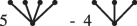
The standard formulation of conditions required to be satisfied for an s-stage Runge–Kutta method to have order p was tabulated by Butcher [1] using an isomorphic mapping from the set of rooted trees having up to p nodes onto polynomial constraints on the coefficients $\{b_i, a_{i,j}, c_j\}$ of a method. For each rooted tree of q nodes, $1\le q\le p$, the constraint is determined in two parts: first, assign sequentially to the nodes of a tree t,  indices i, j, k, ... so that the root has index i, and the tree has q distinct indices. For the elementary differential $\Phi (t)$, assign $b_i$ to the root; for each internal edge $j-k$ occurring, assign $a_{j,k}$ to node k, and to each terminal node l attached to a node k, assign $c_k$. Now, $\Phi (t)$ is equal to the sum over all indices, of the products of the coefficients assigned to all nodes. For example, for the 5-node tree $t_{11}$ (see [3][page 66] for a standard enumeration of trees), the first three parts illustrate this partition to give $\Phi (t)$:

(3)

This constraint is completed by equating $\Phi (t)$ to the reciprocal of an integer-valued function t! identified on this rooted tree. For this, assign the integer 1 to each terminal node of the tree; to each other node, assign 1 plus the total number of its descendent nodes. Then, t! is the product of all integers assigned to the tree. For the example above, $t! = 1\cdot 1\cdot 1\cdot 3\cdot 5 = 15,$ and the full constraint for $t_{11}$ appears in Eq. (3). We now observe that the standard order condition for a general tree t is

$$\begin{aligned} \Phi (t) = \frac{1}{t!}. \end{aligned}$$

(4)

Below, for each tree, we shall specify an alternate order condition to (4) as a linear combination of order conditions $\Phi (t)=1/t!$ for two different trees.

For the column vector, ${{\textbf {e}}}=[1,..,1]^t$, consisting of s ones, each order condition can be represented using vectors {b, e}, a matrix $\textbf{A}$ being strictly lower triangular for explicit methods, and a diagonal matrix ${\textbf {C}}$ for which ${{\textbf {C}}}{{\textbf {e}}}={{\textbf {c}}}$. The left side of each $\Phi (t)$ is a product of ${\textbf {b}}$ followed by products of powers of ${\textbf {A}}$ and ${\textbf {C}}$ selected according to the number of times and positions symbols $a_{i,j}$ and $c_j$ occur in (4), followed by one copy of ${\textbf {e}}$ either for each side branch having at least two contiguous nodes or else for the final branch; the right side remains unchanged. Hence, the order condition for $t_{23}$ can be written as follows:

$${\textbf{bCAC}}^3{{\textbf {e}}} = 1/24.$$

A more general order condition may be written in the form

$$\begin{aligned} {{\textbf {bAC}}}^{k_1}({{\textbf {AC}}}^{l_1}{{\textbf {e}}})..{{\textbf {AC}}}^{k_m}({{\textbf {AC}}}^{l_m}{{\textbf {e}}}){{\textbf {AC}}}^{k-1}{{\textbf {e}}}= 1/t!, \end{aligned}$$

(5)

where t! is specified by the rule above for the right side of a standard order condition. Factors ${{\textbf {AC}}}^{l_i}{{\textbf {e}}}$ arise from side branches of the main tree having two contiguous nodes and can be more general as indicated following (7) below.

Now, we specify a particular set of alternate equivalent order conditions. That is, every method of s stages has order p if and only if its coefficients satisfy both the standard order conditions tabulated by Butcher and this set of alternate order conditions. In fact, there are several ways to select a set of “alternate order conditions.” The approach is to use a (backward) sequence of linear combinations of pairs of standard order conditions to eliminate the rational fraction 1/t! from the right sides of each of the order conditions one by one (excepting only the first-order condition, namely $\Sigma _i \, b_i = 1$).

To specify these alternate order conditions for a method of order p, the strategy for each value of p is to consider the standard conditions in Butcher [3] [page 66] in reverse sequence. Start from tree number $N_p$, and after some alternate conditions have replaced standard order conditions, consider the next standard order condition corresponding to a tree t. If t has at least one branch leaving the root having at least two contiguous edges, the standard order condition will contain a factor $\sum a_{i,j}c_{j}^{k-1}$ (i.e., ${{\textbf {AC}}}^{k-1}{{\textbf {e}}}$) with k maximal. Subtract from this standard order condition for tree t, 1/k times the previous order condition for $t'$ which differs only from that of t by having the stated factor replaced by the factor $c_i^k$ ($={{\textbf {C}}}^k{{\textbf {e}}}$). This yields the alternate order condition

$$ \Phi (t) -\frac{1}{k}\Phi (t') =\frac{1}{I1\cdot I2\cdot k} - \frac{1}{k}\frac{1}{I1\cdot I2}=0, $$

(where $I1,\ I2$ include all factors in the second part t! in (5) not arising from the factor $\sum a_{i,j}c_{j}^{k-1}$), and this constraint is homogeneous in the coefficients. Each of these alternate order conditions will now take the form

$$\begin{aligned} {{\textbf {bAC}}}^{k_1}({{\textbf {AC}}}^{l_1}{{\textbf {e}}})..{{\textbf {AC}}}^{k_m}({{\textbf {AC}}}^{l_m}{{\textbf {e}}}){{\textbf {q}}}^{[k]} = 0, \end{aligned}$$

(6)

where we define stage-order or “subquadrature” expressions as

$$\begin{aligned} {{\textbf {q}}}^{[k]}=({{\textbf {AC}}}^{k-1} - \frac{{{\textbf {C}}}^k}{k}) {{\textbf {e}}}, \quad k=1,..,p-1. \end{aligned}$$

(7)

Formula (6) has different forms depending upon the type of tree it arises from; trees with at least two branches each having two or more contiguous nodes will generate factors such as ${{\textbf {AC}}}^{l_i}{{\textbf {e}}}$ or more general forms (e.g., ${{\textbf {AAC}}}^{l_i}{{\textbf {e}}}$ not shown) and give order conditions of type D below. If there is exactly one single branch leaving the root having at most two contiguous nodes, this order condition will be type C, and hence, equation (6) will be ${{\textbf {bC}}}^{k_1}{{\textbf {q}}}^{[k]}=0.$ A form with three contiguous nodes would have the form ${{\textbf {bC}}}^{k_1}{{\textbf {AC}}}^{k_2}{{\textbf {q}}}^{[k]}=0.$ Otherwise, t will be a bushy tree of $k-1$ nodes attached to the root. For $k>1$, the corresponding quadrature order condition ${{\textbf {Q}}}_k = {{\textbf {bC}}}^{k-1}{{\textbf {e}}}-\frac{1}{k}=0$ will be replaced by the alternate order condition

$$\begin{aligned} k{{\textbf {Q}}}_k - (k-1){{\textbf {Q}}}_{k-1} = 0, \end{aligned}$$

(8)

which may be also be written in the form ${{\textbf {bC}}}^{k-2}(k{{\textbf {C}}}-(k-1){{\textbf {I}}}) {{\textbf {e}}} = 0.$

Each of these alternate order conditions has the form $\beta _i\cdot \alpha _j = 0,\ 2\le i+j \le p$ where $\beta _i$ is a product of b with $i-1$ copies of A and/or C, and $\alpha _j$ is a polynomial in A and/or C of terms up to degree j. Hence, the coefficients of a method of order p must have $\beta _i$ orthogonal to $\alpha _j$, and as each is obtained as a single weighted difference of two standard order conditions, we denote these order conditions as singly orthogonal order conditions (SOOC). Later, we will explore this relationship in more detail, and at that time, the two expressions, $\beta _i$ and $\alpha _j$, will be referred to as the left and right parts of the SOOC respectively. As a simple illustration, the (scaled) difference of the standard order conditions for $t_7$ and $t_5,$

yields the SOOC for $t_7$ as ${{\textbf {b}}}\cdot {{\textbf {q}}}^{[3]} =0$. For this SOOC, ${{\textbf {b}}}$ and ${{\textbf {q}}}^{[3]}$ are the left and right parts respectively.

This procedure changes each of $N_p-1$ standard order conditions to a singly orthogonal order condition (SOOC) by essentially adding a multiple of a standard order condition lower in the sequence, and hence, this process is totally reversible. This establishes the following:

Theorem 1

An s stage method is of order p if and only if its coefficients $({\textbf{b, A,C}})$ satisfy ${\mathbf {b\cdot e}}=1$, and the $N_p-1$ singly orthogonal order conditions.

Proof

For a tree with at least one internal node, consider the “beta-partitioning” [3] [page 48] $t = L(t)*R(t)$ in which R(t) is a subtree obtained by pruning one branch from the root of t. Suppose R(t) contains a penultimate node j which has parent i (possibly the root of t) and $k-1$ terminal nodes as descendants. Now, let $\widehat{t} = L(t)*{R(\widehat{t})}$ be an alternate tree for tree t in which $R(\widehat{t})$ has k nodes attached to node i to replace edge $i-j$ and the $k-1$ terminal nodes of R(t). With this replacement by $R(\widehat{t})$, it follows that in the integers giving $\widehat{t}!$, the value $R(t)!=k\cdot R(\widehat{t})!$. This same replacement also implies that $t!=k\cdot \widehat{t!}\,.$ This in turn implies that, $\Phi (t) = 1/t!$ if and only if $\Phi (\widehat{t}) = 1/\widehat{t!}\,.$ Accordingly, for any particular tree t, we could replace the standard order condition by the requirement that

$$\begin{aligned} \Phi (t) - \frac{1}{t!}= \Phi (t)-\frac{1}{k\cdot \widehat{t!}} = \Phi (t)-\frac{1}{k}\cdot \Phi (\widehat{t}) = 0, \end{aligned}$$

(9)

because the standard order condition for $\widehat{t}$ lies within the remaining (lower sequenced) order conditions. (Observe as above that if R(t) has at most two contiguous nodes, $R(\widehat{t})$ becomes a set of k nodes attached to the root of L(t), and the result holds in the same way.) A similar argument shows that (6) and (8) are necessary for a method to be of order p. Hence, along with the first-order condition, exchanging each standard order condition by the corresponding alternate order condition retains a necessary set of conditions for the method to have order p.

Standard order conditions establish that the singly orthogonal order conditions hold. On the other hand, if the singly orthogonal order conditions hold, the process described above can be reversed starting from the first-order condition and the lowest sequenced SOOC to establish that the standard order conditions hold as well. $\square$

2 Types of order conditions

Order conditions may be partitioned according to the types of problems for which they determine the accuracy of corresponding methods; we characterize four distinct types of order conditions.

To solve $y'=f(x)$, the weights and nodes must satisfy the quadrature conditions, each of which corresponds to a (bushy) tree of $k-1$ nodes each directly connected to the root. To solve linear constant coefficient non-homogeneous problems (C.C. N.-H.) $y' = Ky +f(x)$, order conditions corresponding to tall trees in which each terminal node is connected to the single penultimate node must be satisfied. (A subset of these conditions to solve linear constant coefficient homogeneous problems, $y'=Ky$ corresponding to non-branching trees is not needed here.) To solve linear variable coefficient problems (V.C.), order conditions in which each terminal node is connected to a single node of a tall tree must be satisfied. For all other (non-linear) problems, the order conditions required correspond to trees that have at least two branches each containing two contiguous edges. Typical examples of the four types of standard order conditions are as follows:

• A. Quadrature        $\quad \displaystyle \sum _i b_ic_i^4 = 1/5=\int _0^1 c^4dc$

• B. Linear C.C. N.-H. $\quad \displaystyle \sum _{i,j,k} b_ia_{i,j}a_{j,k}c_k^3 = 1/120$

• C. Linear V.C.        $\quad \displaystyle \sum _{i,j,k} b_i{ c_i^2}a_{i,j}{ c_j}a_{j,k}c_k^2 = 1/120$

• D. Non-linear        $\quad \displaystyle \sum _{i,j,k}{ b_i(a_{i,j}c_j)}(a_{i,k}c_k^2) = 1/36$

Lemma 1

Suppose that the coefficients satisfy either $b_i=0$ or $q_i^{[j]}=0,\ 0\le j\le (p-1)/2$, for each i=1,..,s. Then, each order condition of type D collapses to one of type C.

Proof

For a condition of type D, the corresponding tree has two or more branches from an internal node or the root each having at least two contiguous edges. Assign one maximal branch to be that for which conversion to the alternate form including ${\textbf{q}}^{[k]}$ occurs. Any other branch may contain a factor $\Sigma _la_{i,l}c_l^{j-1}$ with $j\le k$. As this tree has no more than p nodes and each branch excludes the root, it follows that the total number of nodes in the two branches together satisfies $j+j \le j+k \le p-1$, so that $j\le (p-1)/2$. The constraints in the lemma now imply that either $b_i=0$ or else a term $\Sigma _la_{i,l}c_l^{j-1}$ in the recessive branch can be replaced by $c_i^j/j$. A succession of these replacements reduces a type D condition to one of form (6) in which all $l_i$ have vanished, that is type C. $\square$

Now, we illustrate the singly orthogonal forms for each of the four different types of order conditions. These utilize vector–matrix forms and the stage-order expressions:

• A. Quadrature        $\quad ( \textbf{b})\cdot ((5\textbf{C}^4-4\textbf{C}^3) \textbf{e}) = 0$

• B. Linear C.C. N.-H. $\quad ( \textbf{bA})\cdot (\textbf{q}^{[4]}) = 0$

• C. Linear V.C.        $\quad ({ \textbf{bC}^2A})\cdot (\textbf{C q}^{[3]})=({ \textbf{bC}}^2\textbf{AC})\cdot (\textbf{q}^{[3]})=0$

• D. Non-linear              $\quad (\textbf{b}\circ (\textbf{ACe}))\cdot (\textbf{q}^{[3]}) = 0$

For SOOCs of type D, elementwise multiplication of vectors is required, and this is denoted by $\circ$. The orthogonality within each singly orthogonal order condition might be determined in more than one way. Here, a separation into vectors $\beta _i$ and $\alpha _j$ of each SOOC is denoted by $\cdot$ to identify the orthogonality.

Table 2 The numbers of different types of order conditions

Table 2 illustrates how the numbers of the four types of order conditions increase with increasing order. Only the first-order condition $\Sigma _i b_i =1$ does not yield a SOOC, so there are $N_p-1$ singly orthogonal order conditions to solve. (Since $b_i$ appears linearly in each SOOC, vector $\textbf{b}$ can be scaled so that $\Sigma _i b_i=1$ can be solved for $b_1$.)

In contrast to form (5), the right side of each standard order condition can be represented using multiple integrals. For example,

$$\begin{aligned} {{\textbf {bCAC}}}^3{{\textbf {AC}}}^2{{\textbf {e}}}={ {\int _{0}^1 c} \int _0^c {\bar{c}}^3 \int _0^{\bar{c}} {\hat{c}}^2\, d{\hat{c}}\, d{\bar{c}}\, dc}. \end{aligned}$$

(10)

Observe that each occurrence of $\textbf{b}$ or ${\textbf{A}}$ in $\Phi (t)$ is replaced by a definite integral, and each power of C is replaced by the same power of some c. This form is often convenient when formulating the order conditions for direct solution.

3 Solving the order conditions

3.1 Methods for linear constant coefficient non-homogeneous problems

We have already seen that for constraints on $b_i$ and the stage orders, conditions D collapse to conditions C. We shall assume that sufficient conditions hold for this to occur. We now show how to satisfy conditions A and B together for a p-stage method of restricted order p. While such methods can be used to solve a problem of form $y' = Ky + f(x)$, the approach was used to derive classical pairs [11] and will be used here as a skeleton to derive new methods.

Lemma 2

There exist p-stage methods of order p for linear constant coefficient non-homogeneous problems of form

$$y' = Ky + f(x),\quad y(x_0)=y_0,$$

where K is a constant matrix.

Proof

• (a) For p distinct nodes $c_i$, there is a unique solution for $\textbf{b}$ having p entries of

  $$\begin{aligned} \sum _{i=1}^p b_ic_i^{j-1}=\frac{1}{j}, \quad j=1,..,p. \end{aligned}$$

  (11)

• (b) More generally, for p distinct nodes $c_i$, define for each $k=1,..,p$,

  $$\begin{aligned} L_{p+2-k,i}=({\textbf{bA}}^{k-1})_i, \quad i=1,..,p-k+1, \end{aligned}$$

  (12)

  (observing that $b_i = L_{p+1,i},\ i=1,..,p$). Then, for each $k=1,..,p$, unique values $L_{p+2-k,i},\ i=1,..,p+1-k$ can be chosen to satisfy

  $$\begin{aligned} \sum _{i=1}^{p+1-k} L_{p+2-k,i}c_i^{j-1} = \frac{(j-1)!}{(j+k-1)!}, \quad j=1,..,p+1-k. \end{aligned}$$

  (13)

Now, form a strictly lower triangular array L with $L_{p+2-k,i},\ i=1,..,p+1-k,$ making up the elements of row $p+2-k, \ k=p+1,..,2,$ and row $p+1$ containing $L_{p+1,i}=b_i, \ i=1,..,p$. With $L_{p+2-k}$ as defined by (12), it now follows that coefficients $a_{i,j}$ can be computed sequentially up back diagonals of L starting from the right-most diagonal using

$$ a_{q,q-k}=\big (L_{q,q-k} -\sum _{j=q-k+1}^{q-1} L_{q+1,j}a_{j,q-k}\big )/L_{q+1,q}, \quad q=p,p-1,..,k+1,$$

for each $k=1,..,p-1$. This gives the weights $b_i = a_{p+1,i},\ i=1,..,p,$ and the coefficients $a_{i,j},\ 1\le j<i\le p$ of a p-stage explicit Runge–Kutta method that satisfies all of conditions A and B to order p for this restricted class of problems. $\square$

Table 3 provides coefficients of an 8-stage method of order 8 for linear constant coefficient non-homogeneous initial value problems. While order p=8 can be illustrated with simple examples, there is no choice of the arbitrary nodes that will lead to an embedded method of order 7 using the six leading stages of the (8,8) method and only one additional stage. Possibly, other approaches to error estimation could be developed for such methods.

Table 3 An eight-stage method of order 8 for linear constant coefficient non-homogeneous problems

3.2 Explicit (12,8) Runge–Kutta methods for general initial value problems

The motivating theme of this study is to determine the structure of a new family of (13,7-8) pairs of explicit Runge–Kutta methods for general initial value problems (1). Initially, we derive the main 12-stage method of order 8 for such problems. For this, the L-tableau of Lemma 2 has nine rows, and we split it in two ways. First, we insert four new unspecified rows after the first row, and then we insert four columns after the first column. New column values for elements $L_{i,j},$ are inserted so that

$$\begin{aligned} L_{i,j}=0, \quad i=9,..,13,\ j=2,..,5. \end{aligned}$$

(14)

This expanded L-tableau will have the same values in rows 10 to 13 with columns 2 to 8 moved four columns to the right. Values of $a_{i,j}$ for rows 2 to 9 of matrix $\textbf{A}$ of a method will be computed in advance to make stage-order values equal to zero, and as well so that the remaining order conditions of type C will be satisfied. After computing these values for rows 2 to 9 of $\textbf{A}$, values of $L_{i,j}$ in rows 10 to 13 will be used to compute corresponding values of $a_{i,j}$ in these rows using back substitution.

4 Nullspaces

4.1 Mutually orthogonal matrix representations

We now extend the concepts of $\beta _i$ and $\alpha _j$ to be matrices of row and column spaces respectively. For $\beta _i$, there is a very easy extension.

Definition 1

For each i, we define ${\varvec{ \beta }}_i$ to be a matrix of s columns whose rows are vectors of the left parts of SOOCs having products up to i factors.

For example, ${\varvec{\beta }}_i$ may contain $\textbf{b}$ and other rows as appropriate. One possible choice for ${\varvec{\beta }}_4$ is

$$\begin{aligned} { {\widehat{\varvec{\beta }}_4} = \begin{bmatrix} \textbf{b}\\ \textbf{bC}\\ \textbf{bCC}\\ \textbf{bCCC}\\ \textbf{bAA}\\ \textbf{bAAA} \\ \end{bmatrix},} \end{aligned}$$

but this matrix could contain more rows such as $\textbf{bACA}$ or $\textbf{bCAC},$ or from conditions D, $\mathbf (bC)\circ (ACe)$ (where $\circ$ denotes elementwise multiplication). It will be convenient to let $\bar{\varvec{\beta }}_\text {i}$ denote the matrix having a maximum number of different rows so that each entry is a product of up to i factors.

Inconveniently, an extension to ${\varvec{\alpha }}_j$ is more restrictive.

Definition 2

For each j and ${\varvec{\beta }}_j$, we define ${\varvec{\alpha }}_j$ to be a matrix of s rows whose columns are vectors of the right parts of SOOCs of products of up to j factors, such that each column of ${\varvec{\alpha }}_j$ is orthogonal to all rows of ${\varvec{\beta }}_j,$ and we use $\bar{{\varvec{\alpha }}_j}$ to designate a maximum number of different columns.

It turns out that each ${\varvec{\alpha }}_j$ will contain right parts of SOOC conditions B, C, and D, but the only right parts arising from conditions A will be one based on a Legendre polynomial of degree j (orthogonal by integration on the interval [0,1] to all polynomials of lower degree). Hence, matrix ${\varvec{\alpha }}_j$ will not contain ${{\textbf {e}}}=[1,..,1]^t$, but ${\varvec{\alpha }}_1$ could contain $(\textbf{I}-2\textbf{C})\textbf{e}$, and ${\varvec{\alpha }}_2$ could contain $({{\textbf {I}}}-6{{\textbf {C}}}+6{{\textbf {C}}}^2){{\textbf {e}}}$ and/or ${{\textbf {q}}}^{[2]}$. Another example of ${\varvec{\alpha }}_2$ arises from (15) below. An example of ${\varvec{\alpha }}_3$ is

$${\varvec{\alpha }}_3 =[{{\textbf {q}}}^{[2]}, {{\textbf {Cq}}}^{[2]},{{\textbf {Aq}}}^{[2]},{{\textbf {q}}}^{[3]},({{\textbf {I}}}-12{{\textbf {C}}}+30{{\textbf {C}}}^2-20{{\textbf {C}}}^3){{\textbf {e}}}].$$

We observe now that any two matrices ${\varvec{\beta }}_i$ and ${\varvec{\alpha }}_j$ are pairwise orthogonal whenever $1<i\le j$ and $i+j\le p$. Hence, each row of ${\varvec{\beta }}_i$ is a left nullvector of ${\varvec{\alpha }}_j$, and each column of ${\varvec{\alpha }}_j$ is a right nullvector of ${\varvec{\beta }}_i.$

4.2 The nullspace theorem

From these definitions, we have the following:

Theorem 2

For an s-stage method of order p for (1), it is necessary for each $i\le j$ that

$$ {\varvec{\beta }}_i\cdot {\varvec{ \alpha }}_j=0,\quad 2<i+j\le p.$$

$\square$

To derive methods, we might try to characterize coefficients of a method that possess such orthogonality properties. To this end, orthogonality properties of some new methods found using RK-Test-21 have been studied. For these methods, it turns out that there is a surprising two-parameter partitioning of matrix ${\textbf {A}}$ that will be displayed later.

To illustrate how this result is useful, consider the four order conditions for three-stage methods of general order three:

$$\begin{aligned} \begin{array}{l l l} 1.\ {{\textbf {Q}}}^{[1]}=\Sigma _{i=1}^3 b_i -1&{}=0\\[1mm] 2.\ { {\textbf {Q}}^{[1]}}-2{{\textbf {Q}}}^{[2]}=\Sigma _{i=1}^3 { b_i}{ (1-2c_i)}&{}=0\\[0mm] 3.\ 2 {{\textbf {Q}}}^{[2]}-3{{\textbf {Q}}}^{[3]} ={ [b_2\ \ b_3]}\cdot {\begin{bmatrix}c_2(2-3c_2)\\ c_3(2-3c_3)\end{bmatrix}}&{}=0\\[1mm] 4.\ {{\textbf {b}}}\cdot {{\textbf {q}}^{[2]}}=0&{}\\[1mm] \end{array} \end{aligned}$$

(15)

Four solutions with $b_3\ne 0$ exist (see Butcher, [3], p. 63). We can choose

$$\begin{aligned} { {\varvec{\beta }}_1 = \begin{bmatrix} b_1 &{} b_2 &{} b_3 \\ \end{bmatrix}} \ \ and \ \ {{\varvec{\alpha }}_2 = \begin{bmatrix} 1 &{} 0 &{} 0 \\ 1-2c_2 &{}\ \ c_2(2-3c_2)\ \ {} &{}q_2^{[2]} \\ 1-2c_3 &{} c_3(2-3c_3) &{} q_3^{[2]} \end{bmatrix}} ; \end{aligned}$$

these are orthogonal, and ${\textbf {b}} \ne {\textbf {0}}$, so that ${\varvec{\alpha }}_2$ must have rank 2. Hence, ${\varvec{\alpha }}_2$ contains a row or column of zeros, or else has linearly dependent rows, but not all occurrences lead to methods. The four solutions that Butcher reports arise from the last two columns being proportional, the last two entries of row three being zero, and two occurrences of the second column being zero.

5 Twelve stage methods of general order eight

In [11] and [12], the author derived a parametric family of (13,7-8) Runge–Kutta pairs. That is, for a twelve-stage method of order eight, the first ten stages plus one additional 13th stage were used to obtain a second, different method of order seven [11]: the solution of an IVP could be propagated by either method, and the difference of two approximations at each step would provide an estimate of the local truncation error. In practice, this estimate is utilized to select a new stepsize in an attempt to keep the local error small while ensuring that the global error is not too large. In deriving these pairs, the main focus was on the (12,8) method, and that focus continues here. We now assume the nodes are constrained as in Theorem 3(1.) below: this allows stage-order conditions of the algorithm below to be satisfied, and one order condition of type C to be satisfied when three other conditions hold (the proof of which appears in [11]).

With these nodal constraints, coefficients of each (12,8) method of a pair found in [11] were computed using the following algorithm:

• Stage 2: ${q_2^{[1]} =0} \implies a_{2,1}=c_{2}$.                                           SO=1

• Stage 3: $q_3^{[1]}=q_3^{[2]}=0.$                                                        SO=2

• Stage 4: $a_{4,2}=0,\ q_4^{[k]}=0, k=1,2,3.$                                SO=3

• Stage 5: $a_{5,2}=0, q_5^{[k]}=0, k=1,2,3.$                             SO=3

• Stage 6: $a_{6,2}=a_{6,3}=0, q_6^{[k]}=0, k=1,2,3,4.$                   SO=4

• Stage 7: $a_{7,2}=a_{7,3}=0, q_7^{[k]}=0, k=1,2,3,4.$                   SO=4

• Stage 8: $a_{8,2}=a_{8,3}=0, { a_{8,4}\ arb.,\ q_8^{[k]}=0, k=1,2,3,4.}$ SO=4

• Stage 9: $a_{9,2}=a_{9,3}=0, q_9^{[k]}=0,\ k=1,2,3,4,$             SO=4 $L_{13,10}(c_{10}-c_{12})(c_{10}-c_{11})\Sigma _{j=k+1}^9\ L_{11,j}a_{j,k}$$-\Sigma _{j=k+1}^9 L_{13,j}(c_{j}-c_{12})(c_{j}-c_{11})a_{j,k}\ L_{11,10} = 0,\ \ \ \ k=4,5.$

• Weights $b_i=L_{13,i}, \ \ i=1,..,12.$                                     SO=8

• Stages 12, 11, 10: Use back-substitution on $L_{14-k,i}$,            SO=4 $i=13-k,..,1,\ k=2,..,4,$    to get $\ a_{14-k,i}, \quad i=13-k,..,1,\quad k=2,..,4.$

The stage orders (SO) are emphasized for each stage. These anticipate a reduction in the stage orders from SO=4 to SO=3 in stages 7 to 12 in the new methods. This reduction is to be replaced by orthogonality conditions on the corresponding stages, but even more is needed.

Even with this reduction in the stage orders, there remain a number of identities among components of ${\varvec{\alpha }}_4$. Since $a_{i,2}=0,\ i>3,\ a_{i,3}=0,\ i>5,$ and the stage-order constraints on ${{\textbf {q}}}^{[k]}$, for ${{\textbf {e}}}=[1,1,..,1]^T$ and a diagonal matrix $\hat{{\textbf {E}}}_3\ =$ Diagonal[1, 0, 0, 1, 1, .., 1], the following vectors are equal:

$$\begin{aligned} \begin{array}{ll} \hat{{\textbf {E}}}_3{{\textbf {CCCe}}}&{}= 2\hat{{\textbf {E}}}_3{{\textbf {CACe}}}=3\hat{{\textbf {E}}}_3{{\textbf {ACCe}}} =6\hat{{\textbf {E}}}_3{{\textbf {AACe}}}= \\ \hat{{\textbf {E}}}_3{{\textbf {CCAe}}}&{}= 2\hat{{\textbf {E}}}_3{{\textbf {CAAe}}} =3\hat{{\textbf {E}}}_3{{\textbf {ACAe}}} =6\hat{{\textbf {E}}}_3{{\textbf {AAAe}}} \end{array} \end{aligned}$$

Now, premultiplication by $\textbf{C}$ which commutes with $\hat{{\textbf {E}}}_3$ yields

$$\begin{aligned} \begin{array}{ll} \hat{{\textbf {E}}}_3{{\textbf {CCCCe}}}&{}= 2\hat{{\textbf {E}}}_3{{\textbf {CCACe}}}=3\hat{{\textbf {E}}}_3{{\textbf {CACCe}}} =6\hat{{\textbf {E}}}_3{{\textbf {CAACe}}}= \\ \hat{{\textbf {E}}}_3{{\textbf {CCCAe}}}&{}= 2\hat{{\textbf {E}}}_3{{\textbf {CCAAe}}}=3\hat{{\textbf {E}}}_3{{\textbf {CACAe}}} =6\hat{{\textbf {E}}}_3{{\textbf {CAAAe}}}. \end{array} \end{aligned}$$

As well, for $\hat{{\textbf {E}}}_5\ =$ Diagonal[1, 0, 0, 0, 0, 1, 1, .., 1], premultiplication by $\textbf{A}$ and suppressing columns 4 and 5 yields after manipulation

$$\begin{aligned} \begin{array}{ll} \hat{{\textbf {E}}}_5{{\textbf {ACCCe}}}&{}= 2\hat{{\textbf {E}}}_5{{\textbf {ACACe}}}=3\hat{{\textbf {E}}}_5{{\textbf {AACCe}}} =6\hat{{\textbf {E}}}_5{{\textbf {AAACe}}}= \\ \hat{{\textbf {E}}}_5{{\textbf {ACCAe}}}&{}= 2\hat{{\textbf {E}}}_5{{\textbf {ACAAe}}} =3\hat{{\textbf {E}}}_5{{\textbf {AACAe}}} =6\hat{{\textbf {E}}}_5{{\textbf {AAAAe}}}. \end{array} \end{aligned}$$

The latter two sets of identities can be utilized in showing ${\varvec{\beta }}_i\cdot {\varvec{\alpha }}_j=0$ after showing the orthogonality of ${\varvec{ \beta }}_4$ with one column of ${\varvec{\alpha }}_j$ from either set. We refer to the use of lower orders and these as proofs using stage orders.

For each new method of order eight, it is assumed that $b_i=0$ or $q_i^{[k]}=0,\ k=1,2,3,$ for each $i=1,..,s,$ implying that Lemma 1 is valid so that all conditions D collapse to conditions of type C. Otherwise, in contrast to assuming ${{\textbf {q}}}^{[4]}= 0$, it will be assumed that ${{\textbf {q}}}^{[4]}$ lies in the nullspace of $\bar{ {\varvec{\beta }}_4}$. A second non-trivial nullvector of $\bar{{\varvec{\beta }}_4}$ is the Legendre polynomial ${\textbf {J}}_4(\textbf{C})e$ of degree 4 that is orthogonal to all polynomials of lower degree under integration over [0,1]. In particular, observe using order conditions of type A with (10) that

$$ \sum _{i=1}^s b_i c_i^j{{\textbf {J}}}_4(c_i) = \int _{0}^1\ c^j{{\textbf {J}}}_4(c)dc =0,\quad 0\le j\le 3.$$

As well, order conditions of type B imply that ${\textbf{bA}^j\textbf{J}_4(\textbf{C})\textbf{e}=0},\ j=2,3,$ by direct computation, with (12), (13) and (16) so that $\textbf{J}_4(C)e$ lies in the nullspace of $\widehat{\varvec{{\beta }}_4}$. (It might be observed that ${{{\textbf {bA}}}{{\textbf {J}}}_4({{\textbf {C}}})\textbf{e}=0}$ also, but this is not needed yet.) For $\textbf{J}_4(C)e$ to lie in the nullspace of $\bar{\varvec{ \beta }}_4$, we shall show later that the rowspace of $\bar{\varvec{ \beta }}_4$ usually lies in the span of the rows of $\widehat{{\varvec{\beta }}_4}$.

For several examples of these new methods found using RK-Test-21, some properties were determined computationally. These properties guide the statement and proofs for Theorem 3.

• $\bar{{\varvec{\beta }}_4}$ has 15 rows: $\{{\textbf {b}}, {\textbf {bC}}, {\mathbf {bC^2}}, {\mathbf {bC^3}}, {\textbf{bA}}, {\mathbf {bA^2}}, {\mathbf {bA^3}}, {\textbf{bAC}}, {\textbf{bCA}}, {\mathbf {bCA^2}}, {\textbf {bACA}}, {\mathbf {bC^2A}}, {\mathbf {bA^2C}}, {\textbf {bCAC}}, {\mathbf {bAC^2}}\}$ for order conditions of type C

• $\bar{{\varvec{\beta }}_4}$ has 5 rows: $\{\mathbf {b\circ (ACe),b\circ (AACe),b\circ (AC^2e),(bA)\circ (ACe),} \mathbf {(bC)\circ (ACe)}\}$ for order conditions of type D. (Recall that $\circ$ denotes elementwise multiplication.)

• Columns {2,3,4,5} of $\bar{{\varvec{\beta }}_4}$ are columns of zeros, and matrix $\bar{{\varvec{\beta }}_4}$ has rank = 6.

• ${{\textbf {J}}}_4({{\textbf {C}}}){{\textbf {e}}}=({{\textbf {I}}}-20{{\textbf {C}}}+90{{\textbf {C}}}^2-140{{\textbf {C}}}^3+70{{\textbf {C}}}^4){{\textbf {e}}}$ and ${{\textbf {q}}}^{[4]}$ are distinct non-trivial null-vectors of $\widehat{{\varvec{\beta }}_4}$. Hence, its nullspace and that of $\bar{{\varvec{\beta }}_4}$ is spanned by $\{{{\textbf {e}}}_i,\ i=2,..,5,\ {{\textbf {J}}}_4({{\textbf {C}}}){{\textbf {e}}},\ {{\textbf {q}}}^{[4]}\}$.

• The six rows of $\widehat{{\varvec{\beta }}_4}$ are linearly independent, and so they span the rowspace of $\bar{{\varvec{\beta }}_4}$. Hence, the remaining rows are linearly dependent on these.

• When $c_6 = 1/2$, rank (columns 7 to 12 of $\bar{{\varvec{\beta }}_4}$)=5.

• Rank of $\bar{{\varvec{\alpha }}_4}$=5.(This rank might be expected to be 6.)

• Non-trivial columns of ${\varvec{\alpha }}_4$ are ${{\textbf {J}}}_4({{\textbf {C}}}){{\textbf {e}}}$ and ${{\textbf {q}}}^{[4]}$.

Theorem 3

For a 12-stage method:

• 1. Choose 12 nodes with $c_1,c_6,..,c_{12}$ distinct and confined by $c_3=2c_4/3,\quad c_5=c_6(4c_4-3c_6)/(6c_4-4c_6)$, and for $\pi _8(c)=c(c-c_6)(c-c_7)(c-c_8)$, node $c_9$ is chosen so that

  $$ \Big [ \int _0^1 \pi _8(c)\frac{(c-1)^2}{2!} dc \Big ] \Big [ \int _0^1 \pi _8(c)(c-c_9)\frac{(c-1)^2}{2!} dc \Big ] $$
  $$= \Big [ \int _0^1 \pi _8(c)\frac{(c-1)^3}{3!} dc \Big ] \Big [ \int _0^1 \pi _8(c)(c-c_9)\frac{(c-1)}{1!} dc \Big ]. $$

• 2. Choose $a_{i,2}=0,\ i=4,..,12,\ a_{i,3}=0,\ i=6,..,12,\ b_i=0,\ i=2,..,5.$

• 3. Constrain $q_2^{[1]}=0,\ q_3^{[1]}=q_3^{[2]}=0,\ q_i^{[k]}=0,\ i>3,\ k=1,2,3$, and $q_6^{[4]}=0$.

• 4. Constrain stage 9 so that $\Sigma _i b_ic_i^2a_{i,j}=0,\ j=4,5.$

• 5. Choose $L_{i,j}$ by (13) with $L_{i,j}=0,\ j=2,..,5$ (14), and use back-substitution to compute the weights $b_i$ and coefficients of stages 12,11 and 10.

• 6. Choose remaining parameters so $\bar{{\varvec{\beta }}_4}$ is orthogonal to $q^{[4]}$.

Then, for most choices of the arbitrary nodes, the method has order 8.

Proof

The first two nodal constraints of item 1. are needed to allow the several stage-order conditions of items 2. and 3. to be satisfied. The constraints on $c_9$ and item 4. are used to satisfy ${\textbf{bC}}^2{\textbf{AC}}^4\textbf{e}=1/40$ as shown in [11]. Conditions A and B follow from constraints on ${{\textbf {q}}^{[k]}}$ in item 3., together with values of $L_{i,j}$ as specified in item 5. Also, values for $b_i,\ i=2,..,5,$ and those values of $q_i^{[k]}$ assumed to be zero force conditions D to collapse to conditions C. As well, the same values with item 4. imply that columns 2 to 5 of $\widehat{{\varvec{\beta }}_4}$ are all zero.

Next, the rows of $\widehat{{\varvec{\beta }}_4}$ are usually linearly independent. For distinct nodes, linear independence of $\{\textbf{b},\ \textbf{bC},\ \textbf{bCC},\ \textbf{bCCC}\}$ follows from a Vandermonde matrix determined by those values of $b_i$ that are nonzero. To show this, assume $\textbf{bAA}$ is a linear combination of the previous four rows. Hence, for ${\textbf{bAA}}=K_1*{\textbf{b}}+K_2*{\textbf{bC}}+K_3*{\textbf{bCC}}+K_4*{\textbf{bCCC}}$, post-multiplication by ${\textbf{C}}^k{\textbf{e}},\ k=0,..,4,$ with conditions A and B lead to a system of five equations:

$$1/(k+1)(k+2)(k+3) = K_1/(k+1) + K_2/(k+2) + K_3/(k+3) $$

$$+ K_4/(k+4), \quad k=0,..,4.$$

This system in only four unknowns has the unique solution $K_1=1/2,\ K_2=-1,\ K_3=1/2,\ K_4=0$, which yields ${\textbf{bAA}}={\mathbf {b(I-C)}}^2/2$. Letting ${\textbf{A}}_j$ be the $j^{th}$ column of $\textbf{A}$, and observing that $\textbf{A}$ is strictly lower triangular and that the method has 12 stages then ${\textbf{bAA}}_{11}={\textbf{bAAA}}_{11}={\textbf{bAAA}}_{10}=0$. Hence, as $b_{11}(1-c_{11})^2\ne 0$ usually, this leads to a contradiction. Thus, ${\textbf{bAA}}$ is usually linearly independent of $\{\textbf{b},\ \textbf{bC},\ \textbf{bCC},\ \textbf{bCCC}\}$. A similar argument shows that $\textbf{bAAA}$ is usually linearly independent of the four rows and $\textbf{bAA}$. To show this, post-multiplication by ${\textbf{C}}^k{\textbf{e}},\ k=0,..,4,$ of a linear combination for $\textbf{bAAA}$ and stage 11 leads to

$${\textbf{bAAA}}=\frac{c_{11}({\textbf{b}}({\textbf{I}}-{\textbf{C}})^2-2{\textbf{bAA}})}{6}-\frac{{\textbf{bC}}({\textbf{I}}-{\textbf{C}})^2}{6}+\frac{{\textbf{bAA}}}{3},$$

or

$${\textbf{bAAA}}=\frac{{\textbf{b}}(c_{11}{\textbf{I}}-{\textbf{C}})({\textbf{I}}-{\textbf{C}})^2}{6}+(1-c_{11})\frac{{\textbf{bAA}}}{3}.$$

For $\pi _9(c) =c(c-c_{6})(c-c_7)(c-c_8)(c-c_9)$, we obtain using the Lagrange forms, the uniqueness of $b_{10}$ and $L_{13,10}$,

$$b_{10}\pi _9(c_{10})(c_{10}-c_{11})(c_{10}-1) = \int _0^1 \pi _9(c)(c-c_{11})(c-1)dc,$$

and similarly, using $L_{11,10}$

$${\textbf{bAA}}_{10}\pi _9(c_{10})= \frac{1}{2}\int _0^1\pi _9(c)(c-1)^2 dc.$$

Since ${\textbf{bAAA}}_{10}=0$ by the triangularity of $\textbf{A}$, substitution into component 10 of the previous expression leads to

$$0=6{\textbf{bAAA}}_{10}\pi _9(c_{10})= \int _0^1 \pi _9(c)(c-1)\Big \{(c-c_{11})(1-c_{10}) + (c-1)(1-c_{11})\Big \}dc.$$

This requires the linear polynomial in braces to be orthogonal to $\pi _9(c)(c-1)$, and for each viable choice of all nodes except $c_{10}$, this occurs for at most a single viable value of $c_{10}$. Hence, for all other sets of viable nodes, the rowspace of $\widehat{{\varvec{\beta }}_4}$ is a linearly independent set of six rows, and we say that the rows of $\widehat{{\varvec{\beta }}_4}$ usually form a linearly independent set of six rows.

To establish conditions C hold, formulas among $\textbf{A,C,b}$ are used, and these are considered separately. Because values in columns 2 to 5 of $\widehat{{\varvec{\beta }}_4}$ are all zero, and otherwise stage orders are at least three, only order conditions with leading parts in $\widehat{{\varvec{\beta }}_4}$ need to be considered. Formulas (12) and (13) for $L_{i,j}$ for $i=12,13,$ imply that

$$\begin{aligned} \mathbf {bA = b(I-C)}. \end{aligned}$$

(16)

(This is usually known as Butcher’s simplifying condition D(1) [3][p.193].) Observe since $\textbf{A}$ is strictly lower triangular, $(\textbf{bA})_{12}=0$, and as $b_{12}\ne 0$ for a 12-stage method, it follows that $c_{12}=1$, a fact used above and later in (22). Now, substitution of $\textbf{bA}$ or $\textbf{bC}$ from (16) shows that each of $\textbf{bA},\ \textbf{bCA},\ \textbf{bAC},$ $\textbf{bCAA},\ \textbf{bACC}$ lies in the rowspace of $\widehat{{\varvec{\beta }}_4}$. Post-multiplication of (16) by $\textbf{AC}$ shows that the sum $\textbf{bAAC}+\textbf{bCAC}=\textbf{bAC}$ lies in this rowspace; hence, both or neither of $\textbf{bAAC}$ and $\textbf{bCAC}$ lie in this rowspace. Similarly, both or neither of $\textbf{bACA}$ and $\textbf{bCCA}$ lie in this rowspace. Since the nullspace of $\widehat{{\varvec{\beta }}_4}$ contains six linearly independent vectors $\{{\textbf{e}}_i,\ i=2,..,5,\ {\textbf{J}}_4({\textbf{C}}),\ {\textbf{q}}^{[4]}\}$, and has twelve nonzero columns, it has rank at most six and usually contains six linearly independent rows of $\widehat{{\varvec{\beta }}_4}$. Hence, we might expect that the four vectors $\textbf{bAAC}$, $\textbf{bCAC}$, $\textbf{bACA }$ and $\textbf{bCCA}$ will also lie in this rowspace.

We now show that each of these is usually a linear combination of the rows of $\widehat{{\varvec{\beta }}_4}.$ Assume

$${\textbf{bAAC}}=K_1\cdot {\textbf{b}}+K_2\cdot {\textbf{bC}}+K_3\cdot {\textbf{bCC}}+K_4\cdot {\textbf{bAA}}+K_5\cdot {\textbf{bCCC}}+K_6\cdot {\textbf{bAAA}}\,.$$

On post-multiplication by ${\textbf{C}}^k,\ k=0,..,4,$ and solving using order conditions A and B, the solution

$${\textbf{bAAC}}= \frac{{\textbf{bC}}({\textbf{I}} - {\textbf{C}})^2}{2} + K_4\Big ({\textbf{bAA}} - \frac{{\textbf{b}}({\textbf{I}} - {\textbf{C}})^2}{2}\Big ) + K_6\Big ({\textbf{bAAA}} - \frac{{\textbf{b}}({\textbf{I}} - {\textbf{C}})^3}{6}\Big ),$$

for each K$_4$ and K$_6$ is found. Next, for constants

$$F = b_{10}(1 - c_{10})^2,\qquad G = 2{\textbf{bAA}}_{10}(1 - c_{11}),$$

values of $\textbf{bAAC}$ at nodes $c_{11}$ and $c_{10}$ lead to

$$K_4= \frac{(c_{11}- c_{10})F+c_{10}G}{(c_{11}-c_{10})F+G}$$

and

$$ K_6= \frac{3(c_{11} - c_{10})((c_{11}-1)F + G)}{(1 - c_{11})((c_{11} - c_{10})F+G)}.$$

As ${\textbf{bCAC}}={\textbf{bAC}}-{\textbf{bAAC}}={\textbf{bC}}-{\textbf{bCC}}-{\textbf{bAAC}}$, substitution leads to

$${\textbf{bCAC}}=\frac{{\textbf{bC}}({\textbf{I}}-{\textbf{C}}^2)}{2}- K_4\Big ({\textbf{bAA}} - \frac{{\textbf{b}}({\textbf{I}} - {\textbf{C}})^2}{2}\Big ) - K_6\Big ({\textbf{bAAA}} - \frac{{\textbf{b}}({\textbf{I}} - {\textbf{C}})^3}{6}\Big ),$$

with the same set of constants, K$_4$ and K$_6$.

The same approach with an additional order condition of type C (for $\textbf{bACA}$) yields the slightly different formula for

$${\textbf{bACA}}=\frac{{\textbf{b}}({\textbf{I}}-{\textbf{C}})^2({\textbf{I}}+2{\textbf{C}})}{6} + M_4\Big ({\textbf{bAA}} - \frac{{\textbf{b}}({\textbf{I}}-{\textbf{C}})^2}{2}\Big ) + M_6\Big ({\textbf{bAAA}}-\frac{{\textbf{b}}({\textbf{I}}-{\textbf{C}})^3}{6}\Big )$$

with different constants, M$_4$ and M$_6$. For this, stages 11 and 10 imply that

$$M_4= \frac{(c_{11} - c_{10})F + c_{11}G}{(c_{11}-c_{10} )F+G},$$

and

$$M_6=\frac{2(c_{10}-c_{11})F +G}{(c_{11} - c_{10})F+G}.$$

As $\textbf{bCCA}=\textbf{bCA}-\textbf{bACA}=\textbf{b}-\textbf{bC}-\textbf{bAA}-\textbf{bACA}$, on substitution we obtain the representation

$$\textbf{bCCA}=\frac{\textbf{b}(\textbf{I}-\textbf{C})(5\textbf{I}-\textbf{C}+2\textbf{C}^2)}{6}-\textbf{bAA}-M_4\Big (\textbf{bAA}-\frac{\textbf{b}(\textbf{I}-\textbf{C})^2}{2}\Big )$$

$$-M_6\Big (\textbf{bAAA}-\frac{\textbf{b}(\textbf{I}-\textbf{C})^3}{6}\Big ),$$

with the same (second) set of constants, M$_4$ and M$_6$.

If the arbitrary nodes are selected so that the denominators of each pair of K$_4$, K$_6$ and M$_4$, M$_6$ are nonzero, we find that each of $\textbf{bAAC}, \textbf{bCAC}, \textbf{bACA}$ and $\textbf{bCCA}$ lie in the rowspace of $\widehat{{\varvec{\beta }}_4}$. As well, since conditions of type D collapse to conditions of type C, then it follows that each of the vectors ${\textbf{b}}\circ$(${\textbf{ACe}}$)=${\textbf{bCC}}$/2, (${\textbf{bC}}$)$\circ$(${\textbf{ACe}}$)=${\textbf{bCCC}}$/2, (${\textbf{bA}}$)$\circ$(${\textbf{ACe}}$)= ${\textbf{bACC}}$/2, ${\textbf{b}}\circ$(${\textbf{ACCe}}$)=${\textbf{bCCC}}$/3, ${\textbf{b}}\circ$(${\textbf{AACe}}$)=${\textbf{bCCC}}$/6, lie in the rowspace of $\widehat{{\varvec{\beta }}_4}$. Hence, the rowspace of $\bar{{\varvec{\beta }}_4}$ is usually spanned by the rows of $\widehat{{\varvec{\beta }}_4}$.

Now, the orthogonality of $\widehat{{\varvec{\beta }}_4}$ to $\widehat{{\varvec{\alpha }}_4}$ and otherwise stage-order conditions to order 3 imply that all of conditions C hold, and hence, the method has order eight. $\square$

6 Algorithm for new methods

In contrast to the algorithm for classical (12,8) methods above, we begin an algorithm for computing coefficients of nullspace (12,8) methods. Choose values of $a_{7,6}$ and $a_{8,7}$ (to replace $a_{8,4}$ in classical (12,8) methods) arbitrarily. Each nonzero entry of column six of matrix A is equal to a constant plus a multiple of $a_{7,6}$. These multiples are designated as $C1_i,\ i=7,..,12$ with $C1_7=1$, and form the nonzero entries of a right nullvector of the rows of $\widehat{{\varvec{\beta }}_4}$. As well, each nonzero entry of column seven of matrix A is equal to a constant plus a multiple of $a_{8,7}$. More details of these components appear in the next section. Impose the same nodal constraints given in Theorem 3 (these are the same for each (12,8) method of a pair found in [11]), and compute coefficients of a (12,8) nullspace method from:

• Stage 2: ${ q_2^{[1]} =0} \implies a_{2,1}=c_{2}$.                                SO=1

• Stage 3: $q_3^{[1]}=q_3^{[2]}=0.$                                            SO=2

• Stage 4: $a_{4,2}=0,\ q_4^{[k]}=0, k=1,2,3.$                    SO=3

• Stage 5: $a_{5,2}=0, q_5^{[k]}=0, k=1,2,3.$                       SO=3

• Stage 6: $a_{6,2}=a_{6,3}=0, q_6^{[k]}=0, k=1,2,3,4.$              SO=4

• Stage 7: $a_{7,2}=a_{7,3}=0,\ a_{7,6}\ arb.,\ q_7^{[k]}=0, k=1,2,3.$ SO=3

• Stage 8: $a_{8,2}=a_{8,3}=0,\ a_{8,7}\ arb.,\ q_8^{[k]}=0, k=1,2,3,$ SO=3 $q_8^{[4]}=C1_8q_7^{[4]}$

• Stage 9: $a_{9,2}=a_{9,3}=0, q_9^{[k]}=0,\ k=1,2,3,\$              SO=3 $q_9^{[4]}=C1_9q_7^{[4]},$ $L_{13,10}(c_{10}-c_{12})(c_{10}-c_{11})\Sigma _{j=k+1}^9\ L_{11,j}a_{j,k}$ $-\Sigma _{j=k+1}^9 L_{13,j}(c_{j}-c_{12})(c_{j}-c_{11})a_{j,k}\ L_{11,10} = 0,\ \ \ \ k=4,5.$

• Weights $b_i=L_{13,i}, \ \ i=1,..,12.$                            SO=8

• Stages 12, 11, 10: Use back-substitution on $L_{14-k,i}$,       SO=3 $i=13-k,..,1,\ k=2,..,4,$ to get $a_{14-k,i},\ i=13-k,..,1,\ k=2,..,4.$

The intricacies of this algorithm warrant some additional comment. Definitions of bAAA, bAA, bA from those of $L_{i,j},\ i=13,..,10$ imply that $\textbf{bA}^{(k-1)}{{\textbf{q}}^{[4]}}=0,\ k=1,..,3.$ The choice of C1 as a nullvector of $\widehat{{\varvec{\beta }}_4}$ implies that $\textbf{bA}^{(k-1)}\textbf{C1}=0,\ k=1,..,3.$ Now, consider

$$\Sigma _{i=7}^{12}\textbf{bA}^{(k-1)}_i\big \{C1_i-\frac{q_i^{[4]}}{q_7^{[4]}}\big \}=0, \quad k=1,..,3.$$

We have already forced the expression in braces to be zero for each of $i=7,8,9.$ It follows from most if not all values of bAA, bA, b that the matrix must imply all values in braces are zero, and hence, ${\textbf{q}}^{[4]}$ as a multiple of C1 is a nullvector of $\widehat{{\varvec{\beta }}_4}$. As a postnote, we remark that in computing examples of these new nullspace methods, each vector of multiples of $a_{7,6}$ in columns 1, 4, 5, and 6 from rows 7 to 12 is a multiple of the corresponding subvector of ${{\textbf {q}}}^{[4]}$ lying in rows 7 to 12.

In summary, stage orders of stages 7 to 12 are reduced to SO=3, but stage 6 retains SO=4. In place of stage order 4, C1 has been designed as a nonzero nullvector of $\widehat{{\varvec{\beta }}_4}$, and then forced to be a multiple of ${{\textbf {q}}}^{[4]}$. As stated previously after the first algorithm in Section 5, even more is needed.

7 Structure of new methods

Theorem 3 does not quite define an algorithm for the new methods of order eight. When RK-Test-21 was applied using consistent sets of nodes, some problems occurred.

• 1. RK-Test-21 only gave methods when $c_6=\frac{1}{2}$.

• 2. Even for this choice of $c_6$, only a few sets of nodes allowed the RK-Test-21 algorithm in MAPLE to compute coefficients of a new method.

• 3. More detail on making ${{\textbf {q}}}^{[4]}$ orthogonal to $\bar{\varvec{\beta }}_4$ is needed.

These problems motivated an attempt to find an algorithm to directly compute exact coefficients for each method of this new family.

Theorem 4

Assume $\{\mathbf {b, A\ c}\}$, form coefficients of a traditional twelve-stage method of order eight. Assume that the last six columns of $\bar{{\varvec{\beta }}_4}$ is a $20 \times 6$ matrix with rank 5. Define two column and two row vectors by

• $C1_i=0,\ i=1,..,6,\ C1_7=1$, and otherwise, $\textbf{C1}$ is a nonzero solution of ${\bar{{\varvec{\beta }}_4}}.\textbf{C1}=\textbf{0}$.

• $\textbf{R1}$ is the solution of $R1_2=R1_3=0,\ R1_6=1,\ R1_j=0,\ j=7,..,12$, $\Sigma _{i=1}^6 R1_ic_i^{k-1}=0,\ k=1,2,3.$

• $C2_i=0,\ i=1,..,7,\ C2_8=1$, and otherwise, $\textbf{C2}$ is a nonzero solution of ${\bar{\varvec{\beta }}_3}.\textbf{C2}=\textbf{0}$.

• $\textbf{R2}$ is the solution of $R2_2=R2_3=0,\ R2_7=1,\ R2_j=0,\ j=8,..,12,$ $\Sigma _{i=1}^7 R2_ic_i^{k-1}=0,\ k=1,2,3,4.$

Then, for almost all values of  ${\widehat{a_{7,6}}}$ and  ${\widehat{a_{8,7}}},$ and

$$\begin{aligned} {\mathbf {\widehat{A}} }= {\textbf{A}} + {\widehat{a_{7,6}}}~ \mathbf {C1.R1} \ +\ {\widehat{a_{8,7}}}~ \mathbf {C2.R2} \end{aligned}$$

(17)

(where $\mathbf {Ci.Ri}$ defines an outer product), $\{\textbf{b}, \widehat{\textbf{A}}, \textbf{c}\}$ yields another twelve-stage method of order eight.

Proof

The first part of the proof establishes that $\textbf{C1}$ is a right nullvector of $\bar{\varvec{\beta }}_4$, $\textbf{R1}$ is a left nullvector of $\{{\textbf{e}}, \textbf{Ce},{\textbf{C}}^2{\textbf{e}},\textbf{ACe}\}$, $\textbf{C2}$ is a right nullvector of $\bar{\varvec{\beta }}_3$, and $\textbf{R2}$ is a left nullvector of each column vector of $\{{\textbf{e}}, \textbf{Ce},{\textbf{C}}^2{\textbf{e}}, \textbf{ACe},{\textbf{C}}^3{\textbf{e}}, \textbf{ACCe}, \textbf{CACe}, \textbf{AACe}\}.$

Since the matrix equal to the last six columns of $\bar{\varvec{\beta }}_4$ has rank 5, there is a nonzero vector $\textbf{C1}$ with six leading zeros, $C1_7=1,$ and the remaining five values selected so that $\textbf{C1}$ is a right nullvector of $\bar{\varvec{\beta }}_4$. For distinct nodes $\{c_i,\ i=1,4,5\},$ $\textbf{R1}$ can be obtained as specified. As well, for nodes 1 to 6, either $R1_i=0$ or $q_i^{[2]}=0,$ so $\mathbf {R1.ACe}=\mathbf {R1.C}^2{\textbf{e}}/2=0.$ For $C2_i=0,\ i=1,..,7,\ C2_8=1,$ and distinct nodes $\{c_i,\ i=8,..,12\},$ C2 can otherwise be selected so that $\textbf{C2}$ is a right nullvector of $\{{\textbf{b}}, \textbf{bC}, \textbf{bC}^2, \textbf{bAA}\}$. With $\textbf{bA}={\textbf{b}}({\textbf{I}}-{\textbf{C}})$ and the elementwise product $\mathbf {b\circ ACe}$, we find $\textbf{C2}$ is a right nullvector of $\bar{\varvec{\beta }}_3$. Because nodes $\{c_i,\ i=1,4,5,6\}$ are distinct, and $C1_7=1\ne 0,$ with $R2_2=R2_3=0,\ R2_7=1$, values of $R2_i,\ i=1,..,6$ can be selected so that $\textbf{R2}$ is orthogonal to each of $\{\mathbf {e,Ce,C^2e,C^3e}\}$. R2 is orthogonal to the remaining values by the stage-order constraints.

We shall refer to a method with format (17) as a nullspace method. The type A (quadrature) order conditions for the nullspace method are identical to those for the traditional method and hence are valid. We now show that each standard order condition of type B, C, or D for a method with matrix $\widehat{\textbf{A}}$ has the same value as the corresponding order condition for the method with matrix ${\textbf{A}}$. To do this, we consider the left side of a standard order condition (5) with each $\widehat{\textbf{A}}$ replaced by (17). We then expand the resulting expression and consider each term separately. For clarity, we first consider an order condition with only one occurrence of $\widehat{\textbf{A}}$, and for $0\le k+l\le 6$, this gives

$$\begin{aligned} \begin{array}{ll} \textbf{bC}^k \widehat{\textbf{A}}{\textbf{C}}^l{\textbf{e}} &{}= \textbf{bC}^k \textbf{AC}^l{\textbf{e}}+ {\widehat{a_{7,6}}} \textbf{bC}^k. \mathbf {C1.R1.C}^l{\textbf{e}} + {\widehat{a_{8,7}}}\textbf{bC}^k.\mathbf {C2.R2.C}^l{\textbf{e}}\\ &{}= \textbf{bC}^k \textbf{AC}^l{\textbf{e}}. \end{array} \end{aligned}$$

because the latter two terms evaluate to zero. Observe, at least one of $k<4$ or $l<3$: if $k<4,$ then $\textbf{bC}^k. \textbf{C1}=0$, or else $l<3$ and $\mathbf {R1.C}^l {\textbf{e}}=0$, so the second term is zero. As well, at least one of $k<3$ or $l<4,$ and then $\textbf{bC}^k. \textbf{C2}=0$ or $\mathbf {R2.C}^l{\textbf{e}}=0$ respectively, so the third term is zero. For a more general order condition of type B, C, or D in which $\widehat{\textbf{A}}$ must occur more than once, the expansion gives a single term in which only $\textbf{A}$ occurs, or else at least one of the pairs $\textbf{C1,R1}$ and $\textbf{C2,R2}$ occurs at least once. In each term of the expansion, the first occurrence of $\textbf{C1}$ or $\textbf{C2}$ with its orthogonality to $\bar{\varvec{\beta }}_4$ or $\bar{\varvec{\beta }}_3$ respectively will give zero, or else a latter occurrence of $\textbf{R1}$ or $\textbf{R2}$ with its orthogonality to terms in ${\textbf{C}}^k,\ \textbf{AC}^{k-1}, etc.$ will give zero. This will leave exactly an equality of the left side of a standard order condition value from (5) in $\widehat{\textbf{A}}$ to that with the left side of the same order condition of (5) with $\textbf{A}$ replacing each occurrence of $\widehat{\textbf{A}}$. This establishes that each order condition (5) for the method $\{\textbf{b},{\widehat{\textbf{A}}}, \textbf{c}\}$ is satisfied because it is equivalent to the corresponding order condition (5) for the method $\{\textbf{b,A,c}\}$. Hence, coefficients of $\{\textbf{b},{\widehat{\textbf{A}}}, \textbf{c}\}$ yield a new method for each choice of $\widehat{a_{7,6}}$ and $\widehat{a_{8,7}}.$ $\square$

Theorem 5

Suppose a method is chosen by Theorem 4 with $c_6=1/2$ and almost any constants $\widehat{a_{7,6}}$ and  $\widehat{a_{8,7}}$. Then, columns 7 to 12 of $\bar{\varvec{\beta }}_4$ is a $20 \times 6$ matrix of rank 5, and the method is a 12-stage method of order 8.

Proof

It has already been established that the six rows of $\widehat{\varvec{\beta }}_4$ usually span $\bar{\varvec{\beta }}_4$, and that as well, both $\textbf{bAAC}$ and $\textbf{bACA}$ must be in this span. To show that the matrix of the six specified columns of $\bar{\varvec{\beta }}_4$ has rank 5, it is sufficient to show that columns 7 to 12 of the $8 \times 6$ matrix of the rows of $\widehat{\varvec{\beta }}_4$ together with $\textbf{bAAC}$ and $\textbf{bACA}$ has rank 5. Consideration of $\textbf{bAAC}$ and $\textbf{bACA}$ is needed to ensure they exist for $c_6=1/2$ and most choices of the arbitrary nodes. Since $\textbf{A}$ is lower triangular, row reduction of this $8 \times 6$ matrix cascades easily to show that this requirement is equivalent to showing that the $5 \times 3$ matrix RB has rank 2 where the five rows of RB are

• $b_i(c_i-c_{10})(c_i-c_{11})(c_i-1)$,

• $\mathbf{{bAAA}}_{i}$,

• $b_{10}(c_{10}-c_{11})(c_{10}-1)\cdot \mathbf{{bAA}}_{i} - \mathbf{{bAA}}_{10}\cdot b_i(c_i-c_{11})(c_i-1)$,

• $\mathbf{{bAA}}_{i}(c_i-c_{10})$,

• $\mathbf{{bA}}(\mathbf{{C}}-c_{11}I)\mathbf{{A}}_i$,

for $i=7,\ 8,\ 9.$

This requirement is met if each $3 \times 3$ submatrix of RB has a determinant equal to zero. For this, it is sufficient to show the determinant is zero for the three sets of rows $\{1,2,3\},\ \{1,3,4\}$, and $\{1,3,5\}$, for in this case all rows of RB will be linear combinations of rows 1 and 3, and RB will have rank 2. All values needed to compute these rows generically can be found using formulas (12) with (13).

For convenience, let

$$\pi _{6,i}=\Big \{\prod _{j=7}^i c_j\Big \}.\Big \{\prod _{k>j=6}^i (c_j-c_k) \Big \},$$

and $p_5(c_6,..,c_{10})$ = a specific non-factorable multilinear multinomial of degree 5. Using MAPLE, we find

$$Det(\textbf{RB}_{1,2,3}) = \frac{(2 c_6 - 1) (c_{10} - 1)^2 (7 c_6^2 - 7 c_6 + 1) (c_{11} - 1)}{254016000\pi _{6,9}},$$

$$Det(\textbf{RB}_{1,3,4}) = \frac{(2 c_6 - 1) ( 7 c_6^2 - 7 c_6 + 1) (c_{11} - 1)^2 p_5(c_6,..,c_{10})}{71124480000 \pi _{6,10}},$$

$$Det(\textbf{RB}_{1,3,5}) = \frac{(2 c_6 - 1) (c_{10} - 1) (7 c_6^2 - 7 c_6 + 1) (2c_{10}-3c_{11}+1) (c_{11} - 1)}{254016000 \pi _{6,9}}\,.$$

For all three determinants to be zero, the distinctness of nodes 7, .., 12 with $c_{10}\ne 1\ne c_{11},$ implies that $c_6=1/2$, or else $c_6=1/2\pm \sqrt{21}/14$. With either of the latter two choices, some difficulties with applying the algorithm of Theorem 3 arise; otherwise, these latter two choices have been shown to lead to (11,8) methods found by Cooper and Verner [5] and Curtis [6]. Hence, for the methods proposed here, it is necessary that $c_6=1/2$. With this choice, the algorithms of Theorem 3 and Theorem 4 can be applied to find examples in this new family of (8,12) methods. $\square$

Comment Even so, an example for one particular choice of nodes with $c_6=171/410$ (and arbitrary $a_{7,6}$) was found that gave the $6 \times 6$ submatrix from columns 7 to 12 of $\widehat{{\varvec{\beta }}_4}$ the rank 5, the same six columns of all of $\bar{\varvec{\beta }}_4$ the rank 6, and that satisfied all the other nullspace constraints exactly, but led to a 12-stage method only of order 7. (With the single value of $a_{7,6}$ required, the same set of nodes led to a classical 12-stage method of order 8 for any value of $a_{8,7}$.)

8 An embedded method of order seven

For each traditional (12,8) method with $c_6=1/2$, and any value of $\widehat{a_{8,7}}$, the previous sections yield a new family of methods in the parameter $\widehat{a_{7,6}}$. While we have exchanged the freedom to choose an arbitrary value for $c_6$ to make $\widehat{a_{7,6}}$ a parameter, we have derived a new family of explicit Runge–Kutta methods.

For each (12,8) method, it remains to show that a new node, $c_{13} = 1$, and appropriate coefficients for the corresponding thirteenth stage, can be used with the first ten stages to obtain a different (embedded) method of order 7. The weights $\{\widehat{b_i}, \ i=1,..,10,13\},$ provide an order 7 quadrature rule for the nodes $\{c_i, \ i=1,..,10,13\},$ as follows. Choose $\{\widehat{b_i}=0,\ i=2,..,5\},$ and the remaining seven weights may be determined uniquely by integrating the interpolation polynomial on the seven restricted nodes $\{c_i,\ i=1,6,..,10,13\}:$

$$\begin{aligned} \begin{array}{rl} \pi _i(c)&{}=\prod \limits _{\genfrac{}{}{0.0pt}3{j=1,6}{j\ne i}}^{\scriptscriptstyle {10,13}} \displaystyle {\frac{c-c_j}{c_i-c_j}},\\ {\widehat{b}}_i&{}={\int \limits _{0}^1} \pi _i(c) dc . \end{array} \end{aligned}$$

(18)

Coefficients for the new stage will be determined by assuming $a_{13,11}=a_{13,12}=0$, and then using back substitution on

$$\begin{aligned} \begin{array}{rl} ( {\mathbf {\widehat{b}}\textbf{A}})_j &{}=0, \qquad j=2,..,5,\\ ({\mathbf {\widehat{b}}\textbf{A}})_j &{}= \widehat{b_j}(1-c_j),\quad j=1,6,..,10. \end{array} \end{aligned}$$

(19)

Lemma 3

If, for any classical or nullspace twelve-stage method of order eight satisfying $\widehat{\beta }_i\cdot \widehat{\alpha }_j=0,\ i\le j,\ i+j\le 8$, an embedded method is selected using (18) and (19), the embedded method has order seven.

Proof

This proof utilizes the orthogonal properties of the main method to establish that with weights of the embedded method and the new stage, the embedded method has order seven. Equation (18) implies that

$$\begin{aligned} {\mathbf {\widehat{b}}\textbf{C}}^{k-1}{\textbf{e}} = \displaystyle {\frac{1}{k}},\quad k=1,..,7, \end{aligned}$$

(20)

and this equation with (19) implies that

$$\begin{aligned} {\mathbf {\widehat{b}}\textbf{AC}}^{k-1}e = \displaystyle {\frac{1}{k(k+1)}},\quad k=1,..,6. \end{aligned}$$

(21)

Next, we show that ${\mathbf {\widehat{b}}\textbf{A}}$ lies in the span of $\varvec{\beta }_3$. By direct computation with (12), (13), (14) and (21) it follows that

$$\begin{aligned} \Big \{(c_{11}-1){\mathbf {\widehat{b}A}} - {\textbf{b}}(c_{11}{\textbf{I}}-{\textbf{C}})({\textbf{I}}-{\textbf{C}})+2{\textbf{bAA}}\Big \}{\textbf{C}}^k{\textbf{e}} = 0,\quad k=0,..,5. \end{aligned}$$

(22)

Components 11 or 12 of the row vector in braces are zero, and that for $i=13$ is vacuous. As well, the terms for $i=2,..,5,$ are zero because of the restrictions imposed on $\mathbf {b,\ bAA,\ {\widehat{b}} A}$. The remaining submatrix of $\textbf{C}$ using $\{c_i,\ i=1,6,..,10\}$ is Vandermonde with distinct nodes, so it has full rank=6. Accordingly, each remaining component in braces is zero. Hence,

$$\begin{aligned} {\mathbf {\widehat{b}A}}=\frac{1}{c_{11}-1}\Big \{{\textbf{b}}(c_{11}{\textbf{I}}-{\textbf{C}})({\textbf{I}}-{\textbf{C}}) - 2\textbf{bAA}\Big \}, \end{aligned}$$

(23)

implying $\mathbf {\widehat{b}A}$ lies in the rowspace of $\varvec{\bar{\beta }_3}$ and hence is orthogonal to $\varvec{\alpha }_5$.

Now, post-multiply (23) by $\textbf{A}$ to get

$$\begin{aligned} {\mathbf {\widehat{b}AA}} = \frac{1}{c_{11}-1}\Big \{({\textbf{b}}(c_{11}{\textbf{I}}-{\textbf{C}})({\textbf{I}}-{\textbf{C}}){\textbf{A}}-2{\textbf{bAAA}})\Big \}. \end{aligned}$$

(24)

Since the right side lies in the rowspace of $\varvec{\widehat{\beta _4}},$ so also does $\mathbf {{\widehat{b}}AA}$, and so $\mathbf {{\widehat{b}}AA}$ is a left nullvector of $\varvec{\alpha }_4.$

Similarly, $\widehat{b_i},\ (\mathbf {\widehat{b}A})_i=0,\ i=2,..,5$, and post-multiplication of $\mathbf {{\widehat{b}}A}$ in (23) by $\mathbf {AC,\ CA,\ AA,}$ with stage-order constraints imply that $\mathbf {{\widehat{b}}AAC,\ \widehat{b}ACA},$ $\mathbf {\widehat{b}AAA}$ are orthogonal to $\{{\textbf{q}}^{[2]},\ \textbf{Cq}^{[2]},\ \textbf{Aq}^{[2]},\ {\textbf{q}}^{[3]}\}$. Required values of the same three terms post-multiplied by $\textbf{C}^k, k=1,2,3$, and orthogonality elementwise to factors arising from order conditions of type D can be shown by similar arguments. Post-multiplication of (24) by each of $\mathbf {AC,\ CA,\ AA,\ CC}$ gives terms of degree 5, and these lead to the correct values on the right sides. These conditions are sufficient to show that $\mathbf {\widehat{b}}$ and the new stage 13 can be used with the leading ten stages of the method of order 8 to obtain an (embedded) method of order seven by back substitution. $\square$

9 Efficiency of the new methods

The family of new pairs might be considered one that intersects with the family of traditional pairs [11] when $c_6=\frac{1}{2}$. Sets of coefficients for (nearly) optimal traditional pairs have been computed and placed on the author’s website. One possibility is that among the new pairs, the best might be competitive.

It is generally accepted that of any pair of explicit Runge–Kutta methods of successive orders of accuracy, that of higher order is the one accepted for propagation. The difference of the two approximations is used as an estimate of the local error. A good measure of the effectiveness of this process as one that gives accurate solution values to most initial value problems is the 2-norm of the vector of mismatches, $(\Phi (t) - 1/t!)/\sigma (t),$ in coefficients of order conditions of order $p+1$. If the stepsize h is small relative to the interval of solution, this indicates the magnitude of the local error for an IVP. Table 4 reports many well-known (13,7-8) efficient pairs together with three leading nodes, the 2-norm of the coefficients of the higher order leading error term, the largest coefficient (D), and the approximate interval of stability of the higher-order method of each pair. Pairs by this author are indicated by year derived, with characteristic values of the best nullspace method found placed in the last line. Other methods reported appear in Hairer et al. [8] (pages 181-185 - a (12,8-6) pair), Sharp and Smart [10], and as DVERK78 in the MAPLE computing system.

Table 4 Properties of explicit (13,7-8) Runge–Kutta pairs

Appendices

Appendix

This appendix displays an example of a new nullspace (13,7-8) explicit Runge–Kutta pair. The final line in Table 4 states the properties of a near-optimal new pair found. For that pair, the nodes are ${{\textbf {c}}}= {\{0,1/1000,1/9,1/6},5/12,1/2,5/6,$ ${1/6,2/3,19/25,21/25,1,1\}}$, $a_{7,6}=7/3,$ and $a_{8,7}=5/267$. Here, we report a nearby method that has $LTE_2=10^{-5}$, $D=70.386$ and interval of absolute stability of the method of order eight equal to $(-4.567,0]$. To represent this pair, we first state the pair for which $a_{7,6}=a_{8,7}=0$ in Table 5.

Table 5 A nullspace (13,7-8) pair for which the main stage order is three

A different pair arises for almost every choice of $a_{7,6}$ and $a_{8,7}$ although a few discrete choices fail to yield a pair as a result of singularities occurring on the application of the algorithm to derive nullspace pairs. For nodes in Table 5, and almost any choice of $a_{7,6},\ a_{8,7}$, a more general pair is obtained by computing the matrix $\mathbf {\widehat{A}}$ using the following vectors in formula (17):

• Column $C1=[0,0,0,0,0,0,1,-\frac{1}{6},-\frac{343}{243},-\frac{2058}{3125},\frac{343}{1944},\frac{5831}{240},\frac{686}{195}]$

• Row $R1=[-\frac{2}{5},0,0,1,-\frac{8}{5},1,0,0,0,0,0,0,0]$

• Column $C2=[0,0,0,0,0,0,0,1,\frac{2744}{1215},\frac{24696}{78125},-\frac{343}{9720},\frac{5831}{200},\frac{1372}{325}]$

• Row $R2=[\frac{1073}{343},0,0,-\frac{3330}{343},\frac{8352}{343},-\frac{6438}{343},1,0,0,0,0,0,0]$

For a nearly optimal pair with these nodes, choose $a_{7,6}=27/10,\ a_{8,7}=1/72$ in formula (17).

An optimal pair

In contrast to the previous pair, the nodes may be changed to optimize the pair—in the sense that the 2-norm of the local truncation error coefficient discrepancies of the higher-order method is minimized. The final line in Table 4 states the properties of this pair. Slight improvements on this pair are possible by reducing $c_2$ towards zero, but such improvements are marginal. Table 6 records coefficients of $\{{\textbf {b}},\ \varvec{\widehat{b}},\ {\textbf {A}},\ {\textbf {c}} \}$ when $a_{7,6}=0$ and $a_{8,7}=0$ for the optimal pair.

Table 6 A basic nullspace (13,7-8) pair for optimality with main stage order three

A more general pair is obtained when matrix $\mathbf {\widehat{A}}$ is computed with almost any values of $a_{7,6}$ and $a_{8,7}$ using the four following vectors in (17):

• Column $C1=[0,0,0,0,0,0,1,-\frac{1}{5},-8,-\frac{13844844}{1953125},\frac{4279716}{1953125},-\frac{54108}{2315},\frac{3564}{1105}]$

• Row $R1=[-\frac{2}{5},0,0,1,-\frac{8}{5},1,0,0,0,0,0,0,0]$

• Column $C2=[0,0,0,0,0,0,0,1,10,\frac{38073321}{9765625},\frac{1069929}{9765625},-\frac{13527}{463},\frac{891}{221}]$

• Row $R2=[\frac{8}{3},0,0,-\frac{25}{3},\frac{64}{3},-\frac{50}{3},1,0,0,0,0,0,0]$

In particular, we get a nearly optimal pair for the choices of $a_{7,6}=7/3$ and $a_{8,7}=5/267$ using these vectors in (17).

References

Butcher, J.C.: Coefficients for the study of Runge-Kutta integration processes. J. Austral. Math. Soc. 3, 185–201 (1963)
Butcher, J.C.: The numerical analysis of ordinary differential equations. Runge–Kutta and general linear equations. John Wiley & Sons , pp 512 (1987)
Butcher, J.C.: B-Series: an algebraic analysis of numerical methods. Springer/Verlag , pp 310 (2021)
Butcher, J.C.: RK-Test-21: a Runge–Kutta order test. (Web page of J.C. Butcher) (2021) http://jcbutcher.com/node/102
Cooper, G.J., Verner, J.H.: Some explicit Runge-Kutta methods of high order: SIAM. J. Numer. Anal. 9, 389–405 (1972)
Curtis, A.R.: An eighth order Runge-Kutta process with eleven function evaluations per step: Numer. Math. 16, 268–277 (1970)
Fehlberg, E.: Classical fifth-, sixth-, seventh-, and eighth-order formulas with stepsize control: NASA Tech. Rep. NASA 2.7, George C. Marshall Space Flight Center, Huntsville (1968)
Hairer, E., Nørsett, S.P., and Wanner, G.: Solving ordinary differential equations I, Nonsfiff problems, second revised edition. Springer Series in Computational Mathematics 8. Springer–Verlag, Berlin (1993)
Khashin, S. : A symbolic-numeric approach to the solution of the Butcher equations. (2009) http://www.math.ualberta.ca/ami/CAMQ/table_of_content/vol_17/17_3g.htm
Sharp, P.W., Smart, E.: Explicit Runge-Kutta pairs with one more derivative evaluation than the minimum. SIAM J. Sci. Comput. 14, 338–348 (1993)
Verner, J.H.: Explicit Runge-Kutta methods with estimates of the local truncation error. SIAM J. Numer. Anal. 15, 772–790 (1978)
Verner, J.H.: Families of imbedded Runge-Kutta methods. SIAM J. Numer. Anal. 16, 857–875 (1979)
Verner, J.H.: Numerically optimal Runge-Kutta pairs with interpolants. Numer. Algor. 53, 383–396 (2010). https://doi.org/10.1007/s11075-009-9290-3
Zhang, D.K.: Discovering new Runge-Kutta methods using unstructured numerical search. Undergraduate Thesis, Vanderbuilt University, Nashville, Tennessee. (2019) arXiv:1911.00318
Acknowledgements
“RK-Test-21” is an extension of an APL program written on January 1, 1970, jointly by J.C. Butcher and the author to test the order of Runge–Kutta methods; the extension was designed and developed by J.C. Butcher in 2021 to allow direct solution of the Runge–Kutta order conditions by MAPLE. The author thanks J.C. Butcher for providing a copy of the MAPLE code “RK-Test-21” for use in the development of the research in this article and for his encouragement and support during the development of this research.
Author information
Authors and Affiliations
Contributions
The research in this article was developed completely by the author, and the author wrote the complete manuscript and used the MAPLE computing environment with “RK-Test-21” and other code developed and written by the author to compute coefficients in Tables 3, 5, and 6. The author also tabulated the numbers of trees within Table 2.
Corresponding author
Ethics declarations
Ethical approval
Not applicable
Conflict of interest
The author declares no competing interests.
Additional information
Dedicated to Professor J.C. Butcher in celebration of his ninetieth birthday.
Publisher's Note
Springer Nature remains neutral with regard to jurisdictional claims in published maps and institutional affiliations.