Evaluating typical flood risks in Yangtze River Economic Belt: application of a flood risk mapping framework

Abstract

The Yangtze River Economic Belt is one of the three national strategies of China, while flood risk is one of the most important concerns in the development of Yangtze River Economic Belt. In order to decrease the risks caused by floods, complete flood management system and adequate pre-arranged planning are desiderated to be researched in advance. This study considers two typical situations of flood risk, in which one is sluice-control situation in flood detention area and another is dike-break situation in flood-protected area, and proposes a framework for flood risk mapping. The results show that the losses caused by flood hazards are massive both in the two typical cases when extreme floods happen. The economic losses of different indicators are of great difference in flood detention area and flood-protected area, respectively. The framework effectively handles the complex boundaries in the Yangtze River Economic Belt and provides more accurate flood routing information. The evacuation plan module which has been incorporated in the framework also provides informative assistance for emergent action of evacuation under urgent condition.

1 Introduction

Yangtze River Economic Belt (YREB) is defined as an economic zone involving 11 provinces of China along the Yangtze River, the third largest river in the world. The YREB covers an area of nearly 2 million square kilometers and inhabits nearly 40% of Chinese population. The total gross domestic product (GDP) of the YREB contributes over one-third to the entire GDP of China and is considered as the largest economic body in the country. In the year of 2016, the development of YREB is listed as one of three national strategies in the 13th five-year plan of China (Party CCotCC 2016).

Flood is one of the most important limiting and affecting factors for the development of YREB as most of the cities closely located within Yangtze River Basin, and some of which are even in the flood plain. On the one hand, those cities in particular mega cities in the middle and lower reaches of Yangtze River are prone to be affected by floods due to their geographical location (Jongman et al. 2012, 2014; Kundzewicz et al. 2014; Winsemius et al. 2016). For instance, the Wuhan city in the middle reach has been experienced tremendous loss of property and thousands of casualties during two major floods that happened on the year of 1954 and 1998, respectively. On the other hand, massive construction has been implemented in the YREB in recent decades including consolidation of dikes to protect the communities from flood hazards. The Three Gorge Project (TGP), completed in the year of 2008, also plays a very important role in flood control due to its gigantic reservoir storage. In addition, structural measures, nonstructural and management measures are also considered, such as defining different types of flood detention area along with the YREB. Therefore, evaluation of flood risk under the rapid changing conditions is a key task and a critical step in the decision-making process for the development of the YREB.

An effective way to evaluate the flood risk is the utilization of the so-called flood risk mapping (FRM) or flood hazard mapping, which creates easily read and rapidly accessible maps that identify areas at risk of flood. The FRM is designed to increase awareness of the likelihood of flooding among the public, local authorities and other organizations and helps priorities mitigation and response efforts (Ahmadisharaf et al. 2017; Glas et al. 2017; Zhongmin et al. 2008). In addition, the FRM provides a reference for possible land development in flood-prone areas.

Although the scale of the FRM ranges from national map (Kourgialas and Karatzas 2017) to a specific flood-prone/flood detention area (Leopardi et al. 2002; Zhongmin et al. 2008). The procedure for developing the FRM is basically the same and mainly relies on two methods: hydrodynamic simulation and risk analysis. Regarding hydrodynamic simulation, most of the studies used general software (e.g., HEC-RAS, MIKE) to build one-dimensional (1D) hydrodynamic models and two-dimensional (2D) hydrodynamic models (Alho and Aaltonen 2008; Rahmati et al. 2016; Zhang et al. 2016) for calculating basic flood features (e.g., inundation depth and arrival time). The simulations usually equipped with high-resolution digital elevation model (DEM) and geographic information system (GIS) tools for a quick setup of the model. Islam and Sado (2000) used remote sensing data for the historical event of the 1988 flood to develop flood hazard maps. Pelletier et al. (2005) mapped flood inundation by 2D raster-based hydraulic model and satellite image change detection. The above researches that provide successful examples for FRM development of a general case, however, are not practical for the case of YREB due to its complex inner features boundaries (e.g., roads and bridges). Simplification of complex boundary may lead to great error in flood routing simulation and may result in a total unrealistic solution for regional development in the YREB. The functions of these boundaries were of great significance to reflect the real physical process in flood routing.

Regarding risk analysis, a wide spectrum of methods is used such as analytical hierarchical process (AHP)(Rahmati et al. 2016; Stefanidis and Stathis 2013), a multicriteria flood risk assessment approach (Meyer et al. 2009), Monte Carlo-based methods (Apel et al. 2009; Kalyanapu et al. 2012) and remote sensing and GIS-based flood hazard index (FHI) approach (Kabenge et al. 2017). Based on the hydrodynamic simulation and risk analysis, a detailed assessment of flood risk can be drawn and related management measures can be proposed accordingly. Liu et al. (2014) proposes a model-driven decision support system (MDSS) to satisfy the demand of comprehensive flood risk management; a framework in the form of guidelines leading to the formulation of the flood risk management strategies is proposed by Osti (2016); a new conceptual framework for the spatially integrated policy infrastructure is built by Jing and Nedovic-Budic (2016); and Smith et al. (2017) establishes a real-time modeling framework to assess the utility of social media as a data source for flood risk management. Various measures are explored among the studies; however, little attention is given to the preparation of evacuation plan. In itself, the FRM does not cause a reduction in flood risk, and it must be integrated into other procedures, such as emergency response planning and town planning, before the full benefits can be realized. A comprehensive evacuation plan is particularly important to the YREB given its large population and high residential density.

This paper aims to develop a framework of flood risk mapping which is capable of handling complex boundary conditions of computation and addressing the intensive human activities and its interactions with flood hazards in the YREB. Two typical flood risks of sluice-control situation and dike-break situation are used to demonstrate the effectiveness of the proposed framework. The framework also incorporates an evacuation plan module which provides assistance for emergent action of evacuation in urgent condition. The paper is organized in the following. In Sect. 2, the key methodology is described firstly with the overall framework of FRM followed by the description of its components. Then, two cases in the YREB are introduced, and the two typical types of flood risk are considered in Sect. 3. Sections 4 and 5 summarize the results and discuss the FRM development for the two cases. Finally, conclusion is given in Sect. 6.

2 Framework of the FRM

Based on hydrological, administrative, topographic and social economic data, the FRM framework comprises four major components or procedures (Fig. 1): (1) hydrodynamic simulation: to calculate the flood hazards features (e.g., maximum water depth, maximum current speed, inundated range and duration of depth above threshold) in flood plain areas; (2) flood influence analysis: to overlay the economic data, geographic data and flood hazards results to analyze flood influence; (3) evacuation plan: to build an evacuation module and establish the evacuation maps to get the evacuation routes and time when corresponding floods occur; and (4) flood risk mapping: to establish different kinds of flood risk maps within the results of hydrodynamic simulation and influence information/loss data (e.g., maximum water depth map established by maximum water depth results and loss of features/buildings under different water depth levels).

Fig. 1

Framework of flood risk mapping

2.1 Hydrodynamic simulation

River network model (1D), flood routing model (2D) and a 1D–2D dike-break model (i.e., 1D–2D coupled model) are used for simulating flood routing process under various hydrological and terrain conditions. The simulation results include maximum water depth, maximum current speed, duration of depth above threshold, time of flood arrival map and submerged.

2.1.1 1D river network hydrodynamic model

The model is to solve continuous Eq. (1) and momentum Eq. (2) by Abbott implicit discrete method:

$$\frac{\partial \eta }{\partial t} + \frac{\partial Q}{\partial x} = q,$$

(1)

$$\frac{\partial Q}{\partial t} + \frac{\partial }{\partial x}\left( {\alpha \frac{{Q^{2} }}{A}} \right) + gA\frac{\partial \eta }{\partial x} + g\frac{Q\left| Q \right|}{{C^{2} AR}} = 0,$$

(2)

where η represents water level, Q represents discharge, q represents lateral inflow, α is momentum correction factor, g is acceleration of gravity, A represents area of wet cross section, C is Chezy coefficient and R is hydrodynamic radius.

In this study, the MIKE 11 is used for building river network model. Computational grids in MIKE 11 are composed by discharge points and water level points alternately in which water level points are arranged on the center of cross sections (Andrei et al. 2017; Jancikova and Unucka 2015). Between two adjacent water level points, there exists only one discharge point. In order to get numerical solutions, this study used water level points as centers to build implicit format to discretize continuous equation, and discharge points as centers to discretize momentum Equation. 

2.2 2D flood routing hydrodynamic model

In this study, MIKE 21 FM, a module, for computing inundation features and processes of calculated zones by flexible mesh elements (Papaioannou et al. 2016), is used to build 2D flood routing model. The model uses shallow water equation (Morgan et al. 2016; Zavattero et al. 2016) to compute surface flow in two dimensions. The model is based on the solution of the three-dimensional incompressible Reynolds-averaged Naiver–Stokes equations, subject to the assumptions of Boussinesq and of hydrostatic pressure. The integral form can be written as Eqs. (3) and (4):

$$\frac{{\partial \varvec{U}}}{\partial t} + \frac{{\partial \left( {\varvec{F}_{x}^{\text{inv}} - \varvec{F}_{x}^{v} } \right)}}{\partial x} + \frac{{\partial \left( {\varvec{F}_{y}^{\text{inv}} - \varvec{F}_{y}^{v} } \right)}}{\partial y} = \varvec{S}$$

(3)

where $\varvec{F}_{x}^{\text{inv}}$ and $\varvec{F}_{y}^{\text{inv}}$ denote the inviscid and viscous fluxes in x direction of Cartesian coordinates, respectively; $\varvec{F}_{x}^{v}$ and $\varvec{F}_{y}^{v}$ denote the inviscid and viscous fluxes in y direction of Cartesian coordinates, respectively.

$$\begin{aligned} & U = \left[ {\begin{array}{*{20}c} h \\ {h\bar{u}} \\ {h\bar{v}} \\ \end{array} } \right],{\kern 1pt} \begin{array}{*{20}c} {F_{x}^{{{\text{inv}}}} = \left[ {\begin{array}{*{20}c} {h\bar{u}} \\ {h\bar{u}^{2} + \frac{1}{2}g\left( {h^{2} - d^{2} } \right)} \\ {h\overline{{uv}} } \\ \end{array} } \right],} & {F_{x}^{v} = \left[ {\begin{array}{*{20}c} 0 \\ {hA\left( {2\frac{{\partial \bar{u}}}{{\partial x}}} \right)} \\ {hA\left( {\frac{{\partial \bar{u}}}{{\partial y}} + \frac{{\partial \bar{v}}}{{\partial x}}} \right)} \\ \end{array} } \right]} \\ \end{array} , \\ & \begin{array}{*{20}c} {F_{y}^{{{\text{inv}}}} = \left[ {\begin{array}{*{20}c} {h\bar{v}} \\ {h\overline{{vu}} } \\ {h\bar{v}^{2} + \frac{1}{2}g\left( {h^{2} - d^{2} } \right)} \\ \end{array} } \right],} & {F_{y}^{v} = \left[ {\begin{array}{*{20}c} 0 \\ {hA\left( {\frac{{\partial \bar{u}}}{{\partial y}} + \frac{{\partial \bar{v}}}{{\partial x}}} \right)} \\ {hA\left( {2\frac{{\partial \bar{v}}}{{\partial x}}} \right)} \\ \end{array} } \right]} \\ \end{array} , \\ & S = \left[ {\begin{array}{*{20}c} 0 \\ {gh\frac{{\partial d}}{{\partial x}} - \frac{h}{{\rho _{0} }}\frac{{\partial p_{{\text{a}}} }}{{\partial x}} - \frac{{gh^{2} }}{{2\rho _{0} }}\frac{{\partial \rho }}{{\partial x}} + \frac{{\tau _{{sx}} }}{{\rho _{0} }} - \frac{{\tau _{{bx}} }}{{\rho _{0} }} + hu_{s} } \\ {gh\frac{{\partial d}}{{\partial y}} - \frac{h}{{\rho _{0} }}\frac{{\partial p_{{\text{a}}} }}{{\partial y}} - \frac{{gh^{2} }}{{2\rho _{0} }}\frac{{\partial \rho }}{{\partial y}} + \frac{{\tau _{{sy}} }}{{\rho _{0} }} - \frac{{\tau _{{by}} }}{{\rho _{0} }} + hv_{s} } \\ \end{array} } \right] \\ \end{aligned}$$

(4)

where t is the time; h is the total water depth; d is the still water depth; $\bar{u}$ and $\bar{v}$ are the average velocity components in the x and y direction; g is the gravitational acceleration; $\rho$ is the density of water; $p_{\text{a}}$ is the atmospheric pressure; $\rho_{0}$ is the reference density of water; $u_{s}$ and $v_{s}$ are the velocities by which the water is discharged into the ambient water; A is the horizontal eddy viscosity; $\tau_{{{\text{s}}x}}$ and $\tau_{{{\text{s}}y}}$ are the x and y components of the surface wind stresses; $\tau_{{{\text{b}}x}}$ and $\tau_{{{\text{b}}y}}$ are bottom stresses in x and y direction.

Integrating Eq. (3) over arbitrary ith cell and overwriting the equation by using Gauss theorem is given by:

$$\int\limits_{{A_{i} }} {\frac{{\partial \varvec{U}}}{\partial t}} {\text{d}}\varvec{\varOmega}+ \int\limits_{{\partial A_{i} }} \varvec{F} \cdot n{\text{d}}l = \int\limits_{{A_{i} }} \varvec{S} {\text{d}}\varvec{\varOmega}$$

(5)

where A_i denotes the area of the cell $\varvec{\varOmega}_{i}$, n is the unit outward vector normal to boundary $\partial A_{i}$ and ${\text{d}}l$ is the arc elements. In order to avoid numerical oscillation, second-order TVD form is used to solve the model which is given by:

$$\varvec{U}_{{n + {1 \mathord{\left/ {\vphantom {1 2}} \right. \kern-0pt} 2}}} = \varvec{U}_{n} + \frac{1}{2}\Delta t \cdot \varvec{G}\left( {\varvec{U}_{n} } \right),\varvec{U}_{n + 1} = \varvec{U}_{n} + \Delta t \cdot \varvec{G}\left( {\varvec{U}_{{n + {1 \mathord{\left/ {\vphantom {1 2}} \right. \kern-0pt} 2}}} } \right),$$

(6)

where $\varvec{G}_{i} = \frac{1}{{\varvec{\varOmega}_{i} }}\left[ { - \sum\limits_{k} {\left( {\varvec{F}_{i,k}^{\text{inv}} + \varvec{F}_{i,k}^{v} } \right) \cdot \varvec{n}_{i,k} \cdot l_{i,k} } + \varvec{S}_{i} } \right]$, k = 3 or 4, which represents the edges of the ith cell and $\Delta t$ is the time step interval.

2.2.1 1D–2D coupling hydrodynamic model

The 1D model is coupled with the 2D model to simulate the dike-break situation. The standard linkage method combined with dam-break structure module is used. This type of link is useful for connecting a detailed grid into a broader river network. In standard linkage mode, discharge is extracted from the MIKE 11 boundary, centered at time step n + 1/2, and imposed in MIKE 21 FM in a similar way as a MIKE 21 FM source discharge. The discharge from MIKE 11 has an impact on the continuity equation as well as the momentum equation in MIKE 21 FM as with a normal source discharge (DHI 2014b). The first step was to construct a short virtual tributary at dike-break embankment segment, which guarantees the bottom of upstream cross section same as main stream cross section at the link mileage and keeps the bottom of downstream cross section same with the average surface elevation of linked cells in 2D, and then to settle a dam-break structure module in MIKE 11 in the middle of the virtual tributary to simulate a fixed side slope and a short time failure process (Lu et al. 2017). A dam-break module is a composite structure composed of a structure representing the flow over the crest and another structure representing the breach of the dam. Thereinto, the development of the breach uses the “time dependent” mode by settling three parameters: level of the breach bottom, width of the breach bottom and side slope of the breach. In addition, the flow at the dam-break structure is similarly calculated by Weir formula with changeable shape, i.e., the breach increases and the dam crest is shortened (DHI 2014a).

The key parts of establishing hydrodynamic models are illustrated in Fig. 2.

Fig. 2

Schematic diagram of hydrodynamic modeling

2.2.2 Complex boundaries handling techniques

The boundaries of flood detention area/flood-protected area are complex due to the large number of constructive works (e.g., roads, bridges, channels, rivers, houses, arable lands, lakes and woodlands). To deal with the complexity, the boundaries are classified based on the features of different kinds and corresponding techniques are used in the hydrodynamic modeling.

• 1. Woodlands, lakes, arable lands, settlements and water bodies with wide range are considered as different types of land use (as shown in Fig. 3). The hydraulic properties of these features can be defined as roughness which are represented by a set of Manning’s coefficient value M or n. In this study, the set of value n used for settlements, woodlands, arable lands, roads and water bodies are chosen and adjusted as 0.075, 0.060, 0.050, 0.035 and 0.025 based on the research of Chow (1959), Alkema (2003), Sande et al. (2003) and Timbadiya et al. (2014). In Fig. 3, different colors represented different types of land use with different generalized values.

  Fig. 3

  

  Different kinds of land use

• 2. Due to the baffling function in flood routing, railways, highways and national roads which showed linear features are considered in two aspects: (1) to use dike structure module of MIKE 21 FM to generalize these linear features and (2) to refine the grids around the dike structures. The linear features are essentially composed of various points which can be treated as inflexions. The geographical coordinates and the height of the inflexions are the two important parameters of dike structure module. In accord with the handing results of GIS tools, groups of X–Y coordinates and height were extracted. As shown in Fig. 4a, b, the left figure demonstrates distribution of grids using an arbitrary example. The red flexural line is a typical linear structure surrounding with refined triangular grids in mesh file. In the right figure, the red line with several red points represents the graphical representation of dike structure model which has the same coordinates on X–Y plane. In some simple situations which do not require high resolution, modification of the elevation of linear features is an another effective way.

  Fig. 4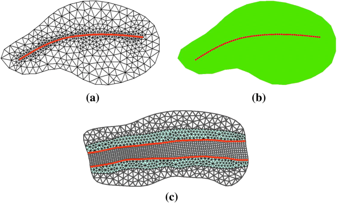

  

  Processing method of linear feature and mixed grids

  Viaducts and soil matrix sections may exist for some sections in highways and, therefore, be considered to. Viaducts are simulated through the dike structure model, while the other sections are generalized as piers which build pier structure model.

• 3. Channels and inland rivers with the function of storing parts of flood and guiding flood routing are considered in the following: (1) to reduce the grids elevation on their location and (2) to refine the local district by using hybrid grids (quadrilateral grids in straight sections and triangular grids in curving sections (as shown in Fig. 4c). It can be find that the river region which is between the two red cross lines has been created by quadrilateral grids. In the middle, the green region refined by triangular grids was transition sections to connect river region with others. The flow directions of quadrilateral grids are relatively regular and structured which suit for expressing channels and inland rivers in the framework. The mixed grids can achieve the target of precise simulation and great cartography.

2.3 Flood influence analysis

After obtaining the results of flood features such as water depth in calculated area, the GIS tools are used: (1) to overlap flood feature layers and socioeconomic data layers through spatial geographical relationship; (2) to calculate and analyze different types and quantities of socioeconomic property; and (3) to set up the relationship between water depth (submerged water yield) and all kinds of property losses. On this basis, combining with water depth and flood duration results, economic losses of different flood situations are evaluated in the following aspects: (1) quantities of administrative regions, areas of cultivated lands and placement places under submerged; (2) mileage of influenced traffic highways and roads; (3) information of influenced administrations, enterprise and public institutions, water conservancy establishments and other major facilities; (4) influenced population; and (5) influenced GDP and financial losses.

It is known that the population is distributed discretely in each administrative region because there are several placement places in each administrative region. And we assume that the population in each placement place is uniform distribution. Finally, the population statistics can be denoted as Eq. (7):

$$P_{e} = \sum\limits_{i}^{n} {\sum\limits_{j}^{m} {A_{i,j} } } \cdot \rho_{i,j}$$

(7)

where $P_{e}$ is flood-hit population, $A_{i,j}$ denotes submerged area of the jth placement place in the ith administrative unit, $\rho_{i,j}$ denotes the density of population of the jth placement place in the ith administrative unit, n is the quantity of administrative units and m is the quantities of placement places.

Loss ratio method can be utilized within five water depth levels ((0 m, 0.5 m], (0.5 m, 1.0 m], (1.0 m, 2.0 m], (2.0 m, 3.0 m] and > 3.0 m) to evaluate and calculate different kinds of major losses which can be described as the form in Eq. (8) including loss of housing, loss of agricultural, loss of enterprise and public institutions property and loss of traffic facilities:

$${\text{Loss}} = \sum\limits_{i = 1}^{n} {\sum\limits_{j = 1}^{m} {\sum\limits_{k = 1}^{k} {f_{i,j,k} \cdot \alpha_{i,j,k} } } }$$

(8)

where $f_{i,j,k}$ denotes the original value of the kth kind of losses of mth placement in nth administrative cell and $\alpha_{i,j,k}$ denotes the loss ratio of the kth kind of losses of mth placement in nth administrative cell. The loss ratio refers to the rate between every kind of property loss and original or normal property, affected by topography, geomorphology, flood features, kind of property, disaster season and emergency measures.

2.4 Evacuation plan

Evacuation plan aims to avoid casualties and minimize the loss of all kinds by preparing evacuation route in advance. The evacuation routes are normally the path between residential areas to designated assembly points/areas. Under the urgent flood conditions, minimal evacuation time is certainly the priority. Corresponding studies which aim at minimizing the evacuation time have been carried out (Wang et al. 2016; Zhang et al. 2016). These studies treated all the transfer roads in the area as a network, and the objective is to minimize the overall transfer time. Therefore, the evacuation model can be described as single objective optimization model. The objective function and corresponding principles including the constraints are written in the following.

• 1. Objective function

  $${\text{mincost}}\,\,T = \sum\limits_{v = 1}^{V} {\sum\limits_{r = 1}^{R} {\sum\limits_{p = 1}^{P} {{\text{cost}}({\text{TR}}_{v,r} )} } } \cdot p$$

  (9)

  where ${\text{cost}}\,T$ is the total transfer time for evacuation, ${\text{TR}}_{v,r}$ represents the rth transfer route prepared for the vth village, ${\text{cost}}(TR_{v,r} )$ reflects the cost time of ${\text{TR}}_{v,r}$ and p is the transfer population scale for the scheme of ${\text{TR}}_{v,r}$

• 2. Constraints

• 1. Accessibility of placements

  The solution set of the terminuses of transfer routes must be found in the feasible region of refuge areas. Each transfer route projected for villages should approach to the regulation placement. It can be described as:

  $${\text{TR}}_{v,r} \in \varPsi_{v}$$

  (10)

  in which $\varPsi_{v}$ is the feasible region of solution set for rth village. The status variable of each unreachable transfer road will be set to zero, i.e., it will be excluded in the model calculation.

• 2. Nearby reallocation of placements

  The evacuation scheduling should consider the principle of proximity by a distance variable. In the case of sufficient accommodation capacity, transfer the evacuees to nearby placements in the first place if the living villages are closed to the placements.

• 3. Prior use of roads principle

  Different level roads have different evacuee spatiotemporal abilities to limit the transfer traffic tools, transfer speeds and time cost. Define the national roads (and above), provincial roads, country roads and county roads from level 1 to level 4. Give precedence to high-level roads for transfer routes in model solution with a static variable of priority.

• 4. Availability of roads

  Flood routing will submerge roads dynamically which influences road selection dynamically. The submerged local roads will be set to unreachable condition in real time by a flag which is set to record the attribute of each road dynamically in each step.

• 5. Coordination of supply and demand constraint

  The mapping relations between evacuees in one village and the placements should be one-to-one or one-to-many by different transfer routes. The solution set should satisfy the demand of each village, i.e., any transfer unit in any village should correspond a certain placement unit. It can be presented as:

  $${\text{Unit}}_{{v,{\text{un}}}} = {\text{Unit}}_{{p,{\text{uc}}}} ,$$

  (11)

  where ${\text{Unit}}_{{v , {\text{un}}}}$ is the unth transfer unit in vth village, ${\text{Unit}}_{{p,{\text{uc}}}}$ is the ucth placement unit in pth placement.

• 6. Capacity constraint of placements

  Each placement should have an upper limit of containable population:

  $$C_{k} = \sum\limits_{{{\text{cr}} = 1}}^{\text{CR}} {p_{\text{cr}} < C_{k}^{ \hbox{max} } } ,$$

  (12)

  where $C_{k}$ is the calculated capacity of the kth placement, $p_{\text{cr}}$ represents the composition of $C_{k}$ and $C_{k}^{ \hbox{max} }$ is the maximum available capacity of the kth placement.

• 7. Consuming time constraint

  $${\text{cost}}({\text{TR}}_{v,r} ) = T_{v,r}^{ \hbox{max} }$$

  (13)

  All evacuees should reach the safe area within limited time. Here, $T_{v,r}^{ \hbox{max} }$ represents the maximum permissive refuge time for vth village.

• 8. Congestion level constraint

  With the advance of the process of refuge and migration, the congestion degree of roads will change. In model, we utilize the classic road weight function representation (Wang 1998; Zheng et al. 2010) to simulate the congestion level in each calculated step.

2.5 Flood risk mapping

The critical step for establishing flood risk maps is layer overlapping by using GIS tools; the following layers are overlapped in the same coordinate system: (1) layer of base map, (2) layer of flood control project, (3) layer of nonstructural measures of flood control, (4) layers of risk factors and (5) layer of social economic data. Except for these spatially distributed information/data, flood risk maps comprise other important information. These informations include three main aspects: (1) The information attached to the entire flood risk maps (e.g., flood characteristic, calculation conditions, probable statistical loss and evacuation information); (2) the information attached to the objects of layers (e.g., population, living conditions and properties); and (3) the corresponding information attached to structural and nonstructural measures of flood control. The process of mapping flood risk maps is presented in Fig. 5.

Fig. 5

Schematic diagram of manufacture of flood risk maps

3 Case and data

Flood detention areas are defined as the regions to temporarily store the flood water by opening the sluice under urgent condition to decrease the water level in the river. Moreover, flood-protected areas should avoid the flood to protect the residents and the properties of various administrative regions. In the planning of YREB, both of them will play the significant roles in flood control. In order to master the possible flood risk to support the construction of YREB, considering the different construction situations and different inner feature boundaries, two typical cases are selected to simulate man-made flood diversion and dike-break flooding situations, respectively, and corresponding flood risk mappings are developed in this study. The first case is Jingjiang flood detention area, which simulates the flood inundation information of sluice-control situation. And the second case is flood-protected area of main dike of the Yangtze River from Hannan to Baimiao, which simulates the flood inundation of dike-break situation.

3.1 Case 1: Jingjiang Flood Detention Area (JJFDA)

Jingjiang flood detention area (JJFDA), which has an area of 921.34 km², is located on the right bank in Jingjiang reach (on the middle reach of Yangtze River) within Gong’an County in Hubei Province (111°14′E–112°48′E and 30°29′N–30°23′N). It is surrounded by Yangtze River at east and Hudu River at west (Fig. 6a). The terrain, higher at north and lower at south, is primarily composed of plain except for the mound at the vicinity of sluice gate. The whole shape resembles a calabash and a neck place (called Majiazui) that is only 2.7 km wide. In possession of 5.4 billion storage capacity for exceedance flood, the referred flood design water level is 42 m. Outside of north gate (NG), the flood design water level is 45.13 m with the corresponding discharge of 7700 m³/s, while the corresponding water level is 45 m of Shashi Stage Gauging Station (SS). The check water level is 45.43 m with the corresponding discharge of 8800 m³/s. Under urgent conditions, the embankment at Lalinzhou (LLZ) can be blasted for flood detention. The JJFDA was used three times in the year of 1954 and stored more than 100 hundred million cubic meter flood water in total.

Fig. 6

Study areas of two cases. a JJFDA and b HBFPA

3.2 Case 2: flood-protected area of main dike of the Yangtze River from Hannan to Baimiao (HBFPA)

Flood-protected area of main dike of the Yangtze River from Hannan to Baimiao (HBFPA) is surrounded by Yangtze River in the east, Hanjiang River in the north and Dongjing River in the southwest (shown in Fig. 6b). The HBFPA covers an area of 4534 km² which include Dujiatai flood detention area (DJT) with the area of 614 km². The terrain is higher in the west/north and lower in the opposite. The average elevation is above 30 m with the highest elevation of around 160 m. A large number of ground works, rivers, lakes and channels are existed in the HBFPA with highways distributed in both vertical and horizontal directions. The HBFPA comprises nearly 270 million resident, 164 thousand hectare cultivated land and 268 billion value industrial production. However, the HBFPA exposes great flood risk due to its geographical location which is intersected with three rivers, and a sophisticated flood risk mapping is needed.

3.3 Modeling data

Hydrologically (discharge and water level) measured data during the flood season in 2010 and 2012 of pivotal controlled steam gauging stations (ZC, SS, CLJ, LS, HK, etc., in Fig. 6a, b) were collected. Design flood process at different frequencies of ZC and SS were collected. In addition, 275 measured cross sections of ZC-CLJ river reach and 108 of LS-HK were collected from hydropower planning survey and design institute. These data were used to build 1D river network hydrodynamic models and calibrate and verify the model parameters. High-precision digital elevation model (DEM) data, digital orthophoto map (DOM) and land-use map in built-up areas were extracted from the database in provincial survey service. These data or maps are used for 2D flood routing models.

Administrative diversion data were collected for formulating the base map of FRMs, which include the administrative borders at country/county levels, and the distribution of county/country government resident and important villages. Besides, refuge areas/safe areas data and parameters of linear features (e.g., highways, dikes and viaduct) were collected for generalizing precise models. Social economic data in each country were collected from local management department or yearbooks in recent 3 years. Finally, detailed road layers were collected for the foundation of the evacuation model with fragmentation.

In this study, ZC ~ CLJ and LS ~ HK river reaches of the Yangtze River were built as main body of 1D river network models in JJFDA case and HBFPA case, respectively. Through calibration and validation, we acquired the precise manning coefficient of value n of ZC ~ CLJ (0.023–0.030 for marginal bank and 0.018–0.022 for river channel), LS ~ HK (0.028/0.023–0.026) and other rivers (0.030–0.038/0.022–0.030), and the results are shown in Fig. 7.

Fig. 7

Parts of the calibration and validation results of the 1D hydrodynamic model. a Hydrographs of water level and b hydrographs of discharge

4 Results

4.1 Results of hydrodynamic simulation

In JJFDA case, we used 1D model to calculate the inflow hydrograph (Fig. 8a) of the entrance BZ and LLZ (which was the red line and yellow line, respectively) under a 0.1% frequency flood of the flood occurred in 1954. For simulating the worst condition, two entrances (NG and LLZ) and no exit were set in the 2D flood routing hydrodynamic model. Localized calculated grids of JJFDA are described in Fig. 9a–c with proposed handling techniques. The figure (a) and (b) demonstrated local grids and refined grids. The figure (c) presented the grids of plain regions.

Fig. 8

Hydrograph of entrances and dike-break position in two cases. a Discharge hydrograph of BZ and LLZ in JJFDA, b discharge hydrograph of XX in HBFPA and c water level hydrograph of XX in HBFPA

Fig. 9

Local calculated grids of JJFDA and HBFPA

In HBFPA case, we aimed at computing and realizing the flood inundation under a 300-year flood of 1954. The design flood hydrograph of LS was set to be inflow boundary in model, while the water level of HK was 29.73 m. The local calculated grids are shown in Fig. 9d, e. The refined and smaller grids represented highways, national roads or other linear structures. In figure (b), the quadrilateral grids generalized the inner rivers and triangular grids for the turning of river. Further, a dam-break model has been utilized to simulate the dike-break situation to couple the 1D model and 2D model through a dike-break model at the place of Xiangxin (XX). In the simulation, the process of dike-break began with a little crack and then developed fast from the top to bottom in the vertical direction within 20 min, gradually expended in the horizontal direction within 2 h, and finally, a trapezoid which was 1000 m wide, 9.94 m high and with a slope value of 1:2.0–1:2.5 took shape. Through the coupling computation of hydrodynamic model, the discharge hydrograph of dike-break is shown in Fig. 8b, c. In figure (b), the blue line represented the hydrograph of cross section of upstream main river channel nearby the dike-break mileage and the green line was the downstream cross section. The red line showed the hydrograph of dike-break section. The volume that flowed into the protected area reached 226.90 hundred million m³, and the volume out of the area (at XX) was about 61.20 hundred million m³.

The flood routing process of JJFDA at 24 h, 48 h, 72 h, 120 h and 180 h is displayed in Fig. 10. The figure (a)–(c) mainly demonstrated the whole process from normal situation to submerged situation. With the peak of flood clipping, the discharge of gate and artificial levee breach decreased gradually. To some degree, the ponding around the entrances gradually moved to downstream region of JJFDA (Fig. 10d, e). In Fig. 10f–k, the reckoning of HBFPA at 24 h, 72 h, 120 h, 240 h, 360 h and 480 h was enumerated in sequential organization. The flood developed from the dike-break position at the southeast corner to the western region and northern region. In final, the submerged area was about 3790 km², and the average water depth was 5.78 m. At last, 84% area of HBFPA had been submerged. Therefore, almost the whole area of Hannan County had been affected. Besides, 90% area of Xiantao County and Hanchuan County or more were submerged by flood. The typical flow field near the breach is shown in Fig. 11. It could be found that the flow was faster near the breach and slower far away. And with the time lapsing, the direction of flow field changed (in Fig. 11d) on the contrary which was in accordance with the flow process of the breach. The intensive arrows in the middle presented the flow field around a linear structure. In addition, the maximum localized distribution of water depth and maximum velocity near the complex boundaries are listed in Table 1, including the places near several different features.

Fig. 10

Flood routing process of two cases. The figure a–e is the process of JJFDA and the figure f–k is the process of HBFPA

Fig. 11

Flow field near the breach of XX at a 24 h, b 120 h, c 360 h and d 840 h

Table 1 The maximum localized distribution of water depth and velocity near the complex boundaries

4.2 Results of flood influence analysis

The layers of land use, highways, national roads, provincial roads, county roads, railways, major enterprises and public institutions, educational organizations and hospitals were taken into account. In JJFDA, the area of submerged administrative region, submerged arable, submerged settlement places and other statistical indexes was calculated in different inundated water depth degrees. The estimated loss and affected data are illustrated in Tables 2 and 3. In the case of HBFPA, 56 towns/villages in 5 counties had been taken into consideration. Through flood influence calculation and analysis, 1029-km-long road and 68.55-km-long railway had been drowned; 196.78 thousands of people affected by flood; and the loss of GDP caused about 80.3 billion yuan (Table 4). The estimated losses of different aspects are presented in Table 5.

Table 2 Statistic of differently affected properties under classification of water depth in JJFDA

Table 3 Losses of different properties in JJFDA

Table 4 Losses of affected different properties in HBFPA

Table 5 Losses of different properties in HBFPA

4.3 Results of evacuation plan

Based on the principle of minimum total transfer time, the evacuation plans were ordered which were drawn as the evacuation maps in Fig. 12. Those indigo points represented the transfer destinations. The red points were transfer units which represented resident of each village and town. The green lines with arrows were on behalf of transfer routes and directions. In the case of JJFDA (Fig. 12a), totally, 179 transfer units of eight towns were divided. Eighty-eight safety platforms, 21 safe areas and six outer safe areas were selected as target places. Eight hundred and thirty-one road sections were prepared. The total consuming time and transfer distance of all units were 71,405 h and 2316 km, respectively. In the case of HBFPA (Fig. 12b), 56 settlements (including three local settlements) for 57 transfer units were selected and divided. Thereinto, the minimum–maximum consuming time was 80.3 min of one unit. The longest transfer route was 79.2 km.

Fig. 12

Schematic diagram of evacuation maps of the two cases. a Local evacuation map of JJFDA and b local evacuation map of HBFPA

4.4 Generation of FRM

Combined the submerged data with the results of flood influence analysis, different kinds of flood inundation map were mapped completely. For instance, the inundation depth map of JJFDA could be drawn as shown in Fig. 13a. In accord with JJFDA case, the inundation depth map of HBFPA was made as demonstrated in Fig. 13b. The figures displayed the flood inundation situation and loss under sluice-control situation and dike-break situation, respectively.

Fig. 13

Examples of FRM in two cases. a Inundation depth map of JJFDA and b inundation depth map of HBFPA

5 Discussion

The complex boundaries played important roles in flood routing which might influence the loss and evacuation routes. As the simulation results are shown (Fig. 10), the linear structures impeded the flood route and direction of movement. The intermittent light color curve represented the roadbeds of highway crossing from top right to middle left of study area. In this curve, the discontinuous places were composed of viaduct which was much higher than general pavement. The simulation results reflect the real situation where the flood bypasses the highway without topping over. In another instance presented in Fig. 10f–i, the flood topped over the dikes of DJT, while in (g) ~ (h), the flood moves along the embankment due to the dikes of inner rivers. These examples showed the effectiveness of the proposed method for handling complex boundaries in YREB.

The result of flood influence analysis in the case of JJFDA showed that the most serious losses were happened in arable. The second place was the loss of houses and production value of industry. The major factor was that the arable had the largest area with great production value. Meanwhile, the crops were too easy to be destroyed by disaster, which was another reason to cause much loss. Compared with other types of properties, the loss of national roads, provincial roads and railways was much less because of small quantity and higher terrain. Besides, most of the enterprises in secondary industry and tertiary industry distributed in the safe regions and their loss rates were less than others and insignificant. In Table 2, it was observed that the inundation depth of 3.0 m was a demarcation of loss. When the depth was lower than 3.0 m, the affected population, area of submerged houses and GDP were not much serious. The special structure of buildings in JJFDA, in which the first floor was empty space with some flood control handling, took great effect. From the results in the HBFPA case, it showed that the loss of industrial output was the most. The rest of losses were in order of agriculture, family possessions, industrial assets and houses. Compared with the losses of the JJFDA case, the possible reason was that the social economic development of flood-protected areas was better than flood detention areas. To a certain degree, the prosperity of industry was one of the key factors which promoted the social economic development. As for different counties, the losses were much different caused by different submerged ranges and inundation depth.

In YREB, 12 key flood detention areas (including JJFDA) have been built or under consideration (Resources CWRCotMoW 2012). Rather than low occurrence probability of dike-break events in flood-protected areas, the flood detention areas have high probability to be used. Combined with flood hazard results, evacuation maps and plans are of great significance to support flood management when necessary, especially in flood detention areas. Based on evacuation model simulation results, consummation and modification of pre-arranged planning for evacuees had been finished. In the results of optimal model, the very smooth roads increased 30 sections and the seriously congested roads decreased 13 sections. Totally, 49 sections promoted road congestion of five congested levels. The optimal results of total consuming time and total distance decreased by 15.36% and by 17.04%. These results have been considered in corresponding management planning of local government department in the year of 2016.

The proposed framework showed effectiveness for preparing flood risk mapping of YREB. The design floods were used as deterministic input which may not cover all the possible flooding scenarios. In the future, a stochastic model for flood generation will be used and uncertainty (e.g., climate change and shape of dike-break) can be considered. A probabilistic model for flood influence analysis will be imported to express flood risk rank (Kalyanapu et al. 2012; Kourgialas and Karatzas 2017) or economic loss (Glas et al. 2017) of hazard zones more intuitive in the maps. However, the framework can be still used in the case with more caution to uncertainty quantification and propagation.

6 Conclusion

An effective framework of flood risk mapping is proposed for YREB, and two typical instances (JJFDA and HBFPA) were used for simulating flood risk under sluice-control and dike-break situation. The results showed that: (1) the highest loss in flood detention area and flood-protected area was loss of agriculture and industrial output, while the lowest was industrial output and housing, respectively; (2) the proposed complex boundary handling techniques effectively simulated more accurate flood routing and hazard information around roads, dikes and rivers in the cases; and (3) the evacuation plan module in the framework can help to improve government urgent planning.

References

Ahmadisharaf E, Kalyanapu AJ, Chung ES (2017) Sustainability-based flood hazard mapping of the swannanoa river watershed. Sustainability 9:1–15. https://doi.org/10.3390/su9101735
Alho P, Aaltonen J (2008) Comparing a 1D hydraulic model with a 2D hydraulic model for the simulation of extreme glacial outburst floods. Hydrol Process 22:1537–1547. https://doi.org/10.1002/hyp.6692
Alkema D (2003) Flood risk assessment for EIA: an example of a motorway near Trento, Italy. Med Phys 34:2593–2594
Andrei A, Robert B, Erika B (2017) Numerical limitations of 1D hydraulic models using MIKE11 or HEC-RAS software—case study of Baraolt River, Romania. In: World multidisciplinary civil engineering-architecture-urban planning symposium-Wmcaus. https://doi.org/10.1088/1757-899x/245/7/072010
Apel H, Merz B, Thieken AH (2009) Influence of dike breaches on flood frequency estimation. Comput Geosci 35:907–923. https://doi.org/10.1016/j.cageo.2007.11.003
Chow VT (1959) In: Chow VT, Harmer ED (eds) Open-channel hydraulics, vol 54, Civil engineering, vol 6, International student edition. McGraw-Hill Book Company, New York, pp 182–192. https://doi.org/ISBN 07-010776-9
DHI (2014a) MIKE 11: a modelling system for rivers and channels user guide. DHI Water and Environment, Hørsholm
DHI (2014b) MIKE FLOOD: 1D–2D modelling user manual. DHI Water and Environment, Hørsholm
Glas H, Jonckheere M, Mandal A, James-Williamson S, De Maeyer P, Deruyter G (2017) A GIS-based tool for flood damage assessment and delineation of a methodology for future risk assessment: case study for Annotto Bay, Jamaica. Nat Hazards 88:1867–1891. https://doi.org/10.1007/s11069-017-2920-5
Islam MDM, Sado K (2000) Development of flood hazard maps of Bangladesh using NOAA-AVHRR images with GIS. Hydrol Sci J 45:337–355. https://doi.org/10.1080/02626660009492334
Jancikova A, Unucka J (2015) DTM impact on the results of dam break simulation in 1D hydraulic models. In: GIS Ostrava compilation surface models for geosciences. Tech Univ Ostrava, Ostrava, Czech Republic, pp 125–136. https://doi.org/10.1007/978-3-319-18407-4_11
Jing R, Nedovic-Budic Z (2016) Integrating spatial planning and flood risk management: a new conceptual framework for the spatially integrated policy infrastructure. Comput Environ Urban Syst 57:68–79. https://doi.org/10.1016/j.compenvurbsys.2016.01.008
Jongman B, Ward PJ, Aerts JCJH (2012) Global exposure to river and coastal flooding: long term trends and changes. Glob Environ Change Hum Policy Dimens 22:823–835. https://doi.org/10.1016/j.gloenvcha.2012.07.004
Jongman B et al (2014) Increasing stress on disaster-risk finance due to large floods. Nat Clim Change 4:264–268. https://doi.org/10.1038/NCLIMATE2124
Kabenge M, Elaru J, Wang HT, Li FT (2017) Characterizing flood hazard risk in data-scarce areas, using a remote sensing and GIS-based flood hazard index. Nat Hazards 89:1369–1387. https://doi.org/10.1007/s11069-017-3024-y
Kalyanapu AJ, Judi DR, McPherson TN, Burian SJ (2012) Monte Carlo-based flood modelling framework for estimating probability weighted flood risk. J Flood Risk Manag 5:37–48. https://doi.org/10.1111/j.1753-318X.2011.01123.x
Kourgialas NN, Karatzas GP (2017) A national scale flood hazard mapping methodology: the case of Greece—protection and adaptation policy approaches. Sci Total Environ 601:441–452. https://doi.org/10.1016/j.scitotenv.2017.05.197
Kundzewicz ZW et al (2014) Flood risk and climate change: global and regional perspectives. Hydrol Sci J 59:1–28. https://doi.org/10.1080/02626667.2013.857411
Leopardi A, Oliveri E, Greco M (2002) Two-dimensional modeling of floods to map risk-prone areas. J Water Resour Plan Manag ASCE 128:168–178. https://doi.org/10.1061/(ASCE)0733-9496(2002)128:3(168)
Liu Y, Zhou J, Song L, Zou Q, Guo J, Wang Y (2014) Efficient GIS-based model-driven method for flood risk management and its application in central China. Nat Hazards Earth Syst Sci 14:331–346. https://doi.org/10.5194/nhess-14-331-2014
Lu C, Zhou J, Jiang Y, Weng Z, Liu Y, Yuan S (2017) Flood routing numerical simulation in jingjiang diversion area based on MIKE FLOOD model. J Basic Sci Eng 25:905–916. https://doi.org/10.16058/j.issn.1005-0930.2017.05.004
Meyer V, Scheuer S, Haase D (2009) A multicriteria approach for flood risk mapping exemplified at the Mulde river, Germany. Nat Hazards 48:17–39. https://doi.org/10.1007/s11069-008-9244-4
Morgan A, Olivier D, Nathalie B, Claire-Marie D, Philippe G (2016) High-resolution modelling with bi-dimensional shallow water equations based codes-high-resolution topographic data use for flood hazard assessment over urban and industrial environments. In: 12th international conference on hydroinformatics (Hic 2016)-smart water for the future, vol 154, pp 853–860. https://doi.org/10.1016/j.proeng.2016.07.453
Osti R (2016) Framework, approach and process for investment road mapping: a tool to bridge the theory and practices of flood risk management. Water Policy 18:419–444. https://doi.org/10.2166/wp.2015.121
Papaioannou G, Loukas A, Vasiliades L, Aronica GT (2016) Flood inundation mapping sensitivity to riverine spatial resolution and modelling approach. Nat Hazards 83:S117–S132. https://doi.org/10.1007/s11069-016-2382-1
Party CCotCC (2016) Outline of Yangtze River economic belt development plan. Party CCotCC, Beijing
Pelletier JD, Mayer L, Pearthree PA, House PK, Demsey KA, Klawon JE, Vincent KR (2005) An integrated approach to flood hazard assessment on alluvial fans using numerical modeling, field mapping, and remote sensing. Geol Soc Am Bull 117:1167–1180. https://doi.org/10.1130/B255440.1
Rahmati O, Zeinivand H, Besharat M (2016) Flood hazard zoning in Yasooj region, Iran, using GIS and multi-criteria decision analysis. Geomat Nat Hazards Risk 7:1000–1017. https://doi.org/10.1080/19475705.2015.1045043
Resources CWRCotMoW (2012) The comprehensive planning of Yangtze River Basin (2012–2030). Changjiang Water Resources Commission of the Ministry of Water Resources, Wuhan
Sande CJVD, Jong SMD, Roo APJD (2003) A segmentation and classification approach of IKONOS-2 imagery for land cover mapping to assist flood risk and flood damage assessment. Int J Appl Earth Obs Geoinf 4:217–229. https://doi.org/10.1016/S0303-2434(03)00003-5
Smith L, Liang Q, James P, Lin W (2017) Assessing the utility of social media as a data source for flood risk management using a real-time modelling framework. J Flood Risk Manag 10:370–380. https://doi.org/10.1111/jfr3.12154
Stefanidis S, Stathis D (2013) Assessment of flood hazard based on natural and anthropogenic factors using analytic hierarchy process (AHP). Nat Hazards 68:569–585. https://doi.org/10.1007/s11069-013-0639-5
Timbadiya PV, Patel PL, Porey PD (2014) A 1D–2D coupled hydrodynamic model for river flood prediction in a coastal urban floodplain. J Hydrol Eng 20:05014017. https://doi.org/10.1061/(ASCE)HE.1943-5584.0001029
Wang W (1998) Urban transportation planning theory and its application. Publishing House of Southeast University, Nanjing
Wang T, Zhou J, Jiang Y, Weng Z, Liu Y, Zhang C (2016) Flood refuge and migration model based on network flow. J Nat Disasters 25:56–64. https://doi.org/10.13577/j.jnd.2016.0107
Winsemius HC et al (2016) Global drivers of future river flood risk. Nat Clim Change 6:381–385. https://doi.org/10.1038/NCLIMATE2893
Zavattero E, Du MX, Ma Q, Delestre O, Gourbesville P (2016) 2d sediment transport modelling in high energy river—application to Var River, France. In: 12th international conference on hydroinformatics (Hic 2016)-smart water for the future, pp 536–543. https://doi.org/10.1016/j.proeng.2016.07.549
Zhang W, Zhou JZ, Liu Y, Chen X, Wang C (2016) Emergency evacuation planning against dike-break flood: a GIS-based DSS for flood detention basin of Jingjiang in central China. Nat Hazards 81:1283–1301. https://doi.org/10.1007/s11069-015-2134-7
Zheng N, Lu F, Duan Y (2010) Dynamic dual graph model for turn delays on road networks. J Image Graph 15:915–920
Zhongmin L, Jun W, Ye S, Zhongbo Y (2008) Study on GIS-based flood risk map for flood detention area. In: Geoinformatics 2008 and joint conference on GIS and built environment: monitoring and assessment of natural resources and environments, Guangzhou, China. SPIE, p 71450F. https://doi.org/10.1117/12.812991
Acknowledgements
This work is supported by the National Natural Science Foundation of China (Nos. 91547208, 51509095 and 51579108).
Author information
Authors and Affiliations
Corresponding author
Rights and permissions
About this article
Cite this article
Lu, C., Zhou, J., He, Z. et al. Evaluating typical flood risks in Yangtze River Economic Belt: application of a flood risk mapping framework. Nat Hazards 94, 1187–1210 (2018). https://doi.org/10.1007/s11069-018-3466-x
Received:
Accepted:
Published:
Issue Date:
DOI: https://doi.org/10.1007/s11069-018-3466-x