
Abstract
Reversible watermarking is a special kind of the lossless data hiding techniques which allows lossless recovering of both the watermark and the host image. In this paper, a new reversible watermarking scheme based on error prediction in Hadamard domain is presented. In the proposed method, the original image is divided into blocks and transformed to Hadamard domain. If a block is in a smooth area, its AC coefficients will be predicted using a linear predictor function. Then the value of error between the original and the predicted coefficient is computed. At last, a watermark bit will be embedded in the error. To reduce the error value, an Adaline neural network is used to determine coefficients of the predictor function. The experimental results show that the proposed method provides higher capacity and quality in comparison to some well-known methods.
1 Introduction
In the recent years, with the dramatic growth of computer networks facilities and dissemination of multimedia contents such as images and videos, etc., the stuff can be easily duplicated and published without the consent of the owner. There are different ways to prevent these problems; digital watermarking is one of these solutions. In a digital image watermarking, a watermark (which can be a logo or a digital signature) is embedded into the host image and the watermarked image is produced. This permits the owner to prove the originality of an image by recovering the watermark from the watermarked image. The main target of the digital watermarking is the invisible and secure embedding of the watermark information into the multimedia content. A digital watermarking consists of two steps: embedding and extraction.
Several classifications of digital watermarking schemes are given in literature. Some ones classify it into robust, fragile and semi-fragile based on the resistance of the watermarking scheme against intentional or unintentional attacks. Robust watermarking methods –as in [2–4, 16]- generally are used for copyright protection and verification of ownership, because they resist most of image processing operations. Fragile watermarking methods –like [13, 19, 35]- are used for content authentication and integrity identification. Semi-fragile watermarking methods –which can be seen in [22, 38]- allow non-malicious modifications, but they are fragile facing malicious attacks. Generally, the images may be manipulated by usual image processing operations, such as compression, which are considered non-malicious. In malicious attack, the meaning of multimedia content changes.
A second classification for digital watermarking schemes is based on the requiring data to extract the watermark [14]. It includes blind, semi-blind and non-blind watermarking methods. Non-blind watermarking schemes need the original image to extract the watermark. A semi-blind watermarking uses some data or parameters of the embedding phase to extract the watermark. However, in a blind watermarking, the original image or any special data or parameters are not used for watermark extraction.
Some special applications such as medical and military imaging systems need to recover both the watermark and the original image exactly [27]. To satisfy this requirement a reversible watermarking scheme may be used. In such a scheme, the original image can be recovered from the watermarked image without any modification, i.e. the original and the recovered images are similar, bit to bit and pixel to pixel.
Similar to other watermarking schemes, a reversible watermarking includes two phases: embedding and extraction. In the embedding phase, a watermark is embedded into the original image. In the extraction phase, the watermark and the original images will be extracted in such a way that the original and the recovered images are equal.
Some reversible methods need to embed some additional data into the original image to assure an exact recovering of the host image. However, the additional data may cause a capacity reduction. There are various classifications for different reversible watermarking methods. One type of classifications is based on the scope in which the watermark is embeded. Spatial domain schemes, transform domain schemes and compression based schemes come under the so-called classification. The literature [6, 11, 12, 15, 18, 20, 24, 25, 28, 29, 34, 40] are in spatial domain. Methods in papers [5, 9, 10, 13, 17, 19, 21, 23, 26, 33, 39] embed the watermark in the transform domain. The works presented in [8, 32] use the compression algorithm to embed the watermark.
In this paper, a new method based on the prediction error in Hadamard domain is proposed. After transferring the original image to Hadamard domain, the watermark bits are embedded in the expanded error between the main and the predicted AC coefficients.
The rest of this paper is organized as follows. In Section 2, some reversible data hiding algorithms are reviewed. Section 3 is devoted to express the motivation of the proposed method. Reversible Hadamard transform, Adaline neural network and prediction error expansion are explained in Section 4. Section 5 presents the proposed data embedding and extraction algorithms. Experimental results are given in Section 6, and finally we conclude in Section 7.
2 Related works
The reversible data hiding was firstly proposed by Barton in 1997 [7]. In the Bartons’s scheme, the bits of watermark signal are first compressed and stored in a bit string. Then, the string is embedded in the multimedia content.
Spatial domain schemes, due to their simplicity and fast implementation, have attracted more attentions. A large number of reversible watermarking methods belong to this group. Ni et al. [28] embedded the watermark by a histogram modification. To do so, the histogram of the original image is computed. Then, the minimum and the maximum values of the histogram are determined (the minimum point of the histogram is the number of pixels with the least repetition in the original image and its maximum point is the number of pixels with the most repetition in the original image). Afterwards, the original image is scanned pixel by pixel. If a pixel value is in the interval between the minimum and the maximum points, the histogram will be shifted to the right by one unit. To embed the watermark, the whole image is scanned again. If the pixel value and the maximum point are equal and the watermark bit is 1, the histogram will be shifted to the right by one unit; otherwise, the histogram is not changed. This method provides acceptable quality but low capacity. Kim et al. [20] proposed a reversible data hiding scheme that modified the difference histogram between sub-sampled images. In their method, the sub-sampled images are generated. Then the watermark is embedded by shifting and modifying the difference histogram. Mahmoudi et al. [6] proposed a prediction based method where the original pixels are predicted by four neighboring pixels, and the secret data is hidden in them.
Coltuc et al. [11] proposed a very fast watermarking method using a reversible integer transform applying to pairs of pixels. This transform is named “Reversible Contrast Mapping” (RCM). The forward and the inverse RCM transforms are as follows.
where \( \left({y}_0,\;{y}_1\right) \) is a pair of pixels in the original image and \( \left({y}_0^{\prime },\;{y}_1^{\prime}\right) \) is a transformed pair of pixels by RCM. The scheme is very fast because it uses a simple transform and does not use any compression algorithm.
Transform domain schemes provide a higher security and at the same time, a higher complexity. These methods usually have a lower capacity in comparison to those of spatial domain. Tian [33] used a Haar wavelet transform to extract high-pass components of an image. He computed the average and the difference values between pairs of pixels using Haar functions. The forward and the inverse of this transform are calculated as follows.
where \( \left({y}_0,\;{y}_1\right) \) is a pair of pixels and L, H are their average and difference, respectively.
In Tian’s method, the watermark is embedded in the expanded difference. This method has high embedding capacity but the two main disadvantages are inappropriate distortion at low capacities and the other is absence of a capacity control caused by embedding a location map [20] (The location map contains the location information of all selected expandable difference values). Al_Qershi et al. [1] proposed a 2-D difference expansion scheme. In this scheme, the original image is divided into blocks of \( 4\times 4 \) pixels. Blocks are transformed by discrete wavelet transform (DWT). Then, the secret data is embedded in expandable blocks (i.e. proper blocks for embedding). In addition, they use some characteristics such as standard deviation and uniformity to enhance the visual quality. Du et al. [13] proposed a DCT based reversible watermarking. In this method, the original image is divided into \( 8\times 8 \) non-overlapping blocks. After applying DCT to each block, the high frequency coefficients are selected to embed the watermark. If the watermark bit is ‘0’, the current coefficient will not be changed; otherwise, it will be increased by a fixed value. Their method has low capacity because just one bit of the watermark is embedded in each block. Gao et al. [17] suggested integer DCT-based method. They computed the energy of each \( 8\times 8 \) block which formerly has been transformed by DCT. Then they selected the suitable blocks using a proper threshold value. Lin [23] used DCT to transform the original image. In order to leave a space for hiding the watermark, the positive coefficients are shifted to the right and the negative ones to the left. Note that both two coefficients are around zero.
Compression based schemes use a lossless compression algorithm to compress the payload bits. Since, these methods use one of compression algorithms, they are complicated in computing. However, they provide high capacities. Celik et al. [8] proposed a new method using a quantization function to quantize the pixel values. The reminders of the quantization operation are compressed with a lossless compression algorithm called CALIC [37]. These compressed reminders are then attached to the watermark bits. Finally, the whole is embedded in the original image. Thodi et al. [32] offered a prediction based reversible embedding method. In this method, pixel values are predicted using their neighboring pixels. The suitable locations are selected by setting a threshold on the magnitude of the predicted errors. All the selected locations are coded in a location map. The location map is compressed by a lossless compression algorithm. After attaching the watermark bits to the compressed location map, the whole will be embedded in the original image based on an expanded error.
3 Motivation
As mentioned in section 1, fragile watermarking is commonly used for content authentication and tamper detection in digital multimedia. In this paper, we proposed a new fragile reversible watermarking in transform domain to authenticate the content and to recognize the tamper. This method is a blind one, as well. We neither need any special data nor any parameter to extract the watermark and to recover the original image.
Most proposed reversible watermarking techniques in transform domain use the wavelet transform [33, 39] while some methods use DCT [13] or integer DCT [17]. However, these methods are not completely successful. As, they cannot satisfy both two capacity and quality needs. This article presents a new method in the transform domain resulting in acceptable capacity of payload bits and at the same time, good quality of the watermarked image. The point is that, in this method, the reversible Hadamard transform is used to commute the original image. Based on our experimental results, the reversible Hadamard transform gives the better results in comparison to others’ like DCT, integer DCT or DWT.
Moreover, some transform domain methods directly hide the secret data in the LSB (Least Significant Bit) of the transform coefficients [1, 23]. Direct embedding in coefficients causes the reduction of visual quality. Therefore, these methods have to decrease the amount of embedding capacity to improve the visual quality. The proposed method is highly recommended to achieve a good trade-off between the capacity and the quality in transform domain. To do so, AC coefficients are predicted by a predictor function. Then the watermark bits are hidden in the LSB of each error (which is between the main and the predicted AC coefficients). Thus, by embedding the watermark in the error instead of direct embedding, the visual quality will be improved.
The predictor function, which is used to predict the AC coefficients, is a linear one. The coefficients of the predictor are important to predict the AC coefficients accurately. Here, we use the Adaline neural network to find better coefficients due to its use of the image local information. Although it is possible to use a constant number, it does not provide a suitable prediction. However the results of both two mentioned ways, to determine the prediction coefficient, are reported in our paper.
4 Basic concepts
In the rest of the article, we describe a reversible watermarking method based on a prediction error in Reversible Walsh-Hadamard domain. The AC coefficients of a Reversible Walsh-Hadamard transform are predicted by a linear predictor function –as it mentioned before. The coefficients of the predictor function can be determined by an Adaline neural network for more accurate prediction. The watermark bits are embedded in the expanded error between the main and the predicted AC coefficients.
Before explaining the proposed method, let us review Reversible Walsh-Hadamard transform, Adaline neural network and the prediction error expansion.
4.1 Reversible Walsh-Hadamard transform
The Walsh-Hadamard transform is one of the widely used transforms in the signal and the image processing. It is a non-sinusoidal transform based on the Hadamard matrix [31]. The Hadamard matrix of the n order is the \( \left(\pm 1\right) \)_matrix with the size of \( n\times n \) (\( {H}_n \)) satisfying the orthogonality condition:
where T is a transposition sign, I n is an identity matrix of the n order.
One of the well-known Hadamard matrices is the Silvester matrix, which is a matrix of order 2k and can be recursively generated as follows:
The Hadamard transform of an n × n unitary matrix, I n , is defined by:
According to the Eq. (6), reversible Walsh-Hadamard transform matrices are recursively defined as follows:
The forward and inverse reversible Walsh-Hadamard transform matrices of order 4 are shown in the following matrices [30]:
4.2 Adaline neural network
Widrow and Hoff developed an Adaptive Linear Neuron (ADALINE) in 1960 [36]. Adaline is a single layer neural network with multiple nodes in a way that each node can be multiple inputs and results one output. It consists of a weight, a bias and a summation function.
This network is shown in the Fig. 1. As one can see in this figure, I is the input vector. W is the weight vector and O is the output. The output can computed by the following equation:
where R is the number of elements in the input vector.

Adaline neural network
In this network, the weights are updated as follows:
where η is the learning rate, and, d is the desired output.
The error between the computed output and the desired output should be converged to the least squares error which is:
This problem can be solved in another way. So, the Eq. (9) can be rewrite as follows:
We want to obtain the weights, so we can multiply I T in the Eq. (12) and compute the weights, directly; where I T is the transpose of input vector.
where \( {\left(\alpha \right)}^{-1} \) is the inverse of α.
4.3 Prediction error expansion
In the prediction error expansion, a pixel value is predicted using its neighboring pixels [32]. Then, the error between the main and the predicted value of the pixel is computed. Finally, the watermark is embedded into the empty LSB of the shifted error; this called error expansion. This method is described below in detail.
As a first step, a pixel value is predicted by using its adjacent pixels. Then, the error between the original and the predicted values of the pixel is calculated by the following equation:
where y, ŷ are the original and the predicted values of the pixel, respectively.
The binary representation of e is computed. Then it is shifted to the left by one bit to create an empty LSB, into which the watermark bit is embedded. The binary representation of e and the watermarked error is computed as below:
where b 0 is the LSB and l is the bit length of e. e′ is the expanded error and i is the watermark bit.
The expanded error and the predicted pixel values are added to obtain the watermarked pixel value by the following equation:
To extract the watermark bit and recover the original pixel value, the value of the watermarked pixel is predicted the same as of the embedding watermark. Then, the error between the watermarked and the predicted value of the pixel is computed and the watermark bit is extracted as follows:
where the expanded error is e′ = y′ − ŷ.
The original error and the main value of the pixel are computed by using the following equations.
5 Proposed method
The proposed scheme consists of two phases: the embedding and the extraction.
-
In the embedding phase, the original image is divided into \( 4\times 4 \) non-overlapping blocks. Then, a reversible Hadamard transform will be applied to each block. After that, the AC coefficients are predicted. At last, the watermark bits are embedded in the computed errors between the original and the predicted AC coefficients.
-
In the extraction phase, the reverse of the embedding process is repeated roughly, i.e. the watermarked image is divided into \( 4\times 4 \) non-overlapping blocks. After transferring blocks to Hadamard domain, the watermarked coefficients are predicted. Then the watermarked errors are calculated. The extraction of watermark bits is followed by the previous step. Finally, the original image will be recovered.
The flowchart of the proposed method is given by Fig. 2.

The flowchart of embedding and extraction algorithm
Before working on the two phases of the proposed method, it is highly recommended to have a look over the distortion control, which is explained extensively below:
The distortion control is a way of avoiding the probable distortion. Embedding the watermark into the original image may create the invalid values for some pixels. The occurrence of overflow and underflow are some factors of damaging the watermarked image.
The two terms (the overflow and the underflow) are defined in the following. For an 8-bit grayscale image, if the value of a pixel is more than the upper bound of pixel values (i.e. 255), overflow will occur while underflow will occur if the value of a pixel is less than the lower bound of pixel values (i.e. 0).
In this article, to decrease the distortion and to prevent the over/underflow in the watermark embedding phase, we select a smooth block as an expandable one (a block which is proper to embed the watermark). As it will be mentioned in section 5.1.1, the AC coefficients are predicted using the DC values of a \( 3\times 3 \) neighbor block. If a block places in a smooth area, the prediction of AC coefficients will be more accurate. Since, the values of pixels are close to each other in the smooth area. But in the edge area the values of pixels are so varied and the values of errors will be increased.
Avoiding of the over/underflow can be achieved by choosing a proper threshold. If the difference between a pixel and its neighbors in a block is less than a predefined threshold, the watermark bit will be embedded; otherwise, the watermark bit won’t be:
where Th is a predefined threshold value. Pixel and pixel_neighbor are the current and the neighbor pixels values, respectively.
Even if the difference between a pixel of a block and its neighbors is more than the threshold, no watermark will be embedded in the block. Therefore, the smooth blocks are detected afterward the watermark bits are embedded.
5.1 Watermark embedding phase
The embedding process is performed in the transform domain. At first, the original image is divided into \( 4\times 4 \) non-overlapping blocks. Then blocks are commuted to transform domain by the reversible Hadamard transform. Before embedding the watermark bits, the first and the second blocks are considered to embed the length of the watermark. Then other blocks are scanned to specify the smooth ones by the use of Eq. (21). To recognize the expandable (smooth) blocks, one of the AC coefficients is considered as a detection coefficient. The location of the detection coefficient in a block is indicated in the Fig. 3. According to this figure, \( {AC}_{22} \) is the detection coefficient. In this case, two manners may occur:

The location of AC coefficients
-
1)
If the scanned block is an expandable one, a bit ‘1’ will be embedded in the expanded error of the detection coefficient and the watermark bits will be embedded in the expanded errors of other AC coefficients of this block, afterward;
-
2)
If not, a bit ‘0’ will be embedded in the expanded error of the detection coefficient and no watermark bit will be embedded in this block.
To embed a bit of payload in an AC coefficient, the AC coefficient is predicted by a linear predictor function. Then, the error between the main and the predicted AC coefficient is computed. Finally, the bit of payload is embedded in the expanded error. Note that no watermark is embedded in the DC coefficients, which means these coefficients won’t change. And no watermark is embedded in the marginal blocks of the image.
In this phase, we explain the embedding algorithm step by step. Then we clarify how to determine the coefficients of the predictor function.
5.1.1 Watermark embedding algorithm
We describe the embedding algorithm in the following steps:
-
Step 1
The original image is divided into \( 4\times 4 \) non-overlapping blocks. The reversible Hadamard transform is applied to each block for commuting them to the transform domain. As mentioned previously, marginal blocks of the image are not used to embed the bits of payload. Therefore, we start from the second row and column of blocks for embedding.
-
Step 2
The length of the watermark is embedded in the first and the second blocks by the proposed algorithm. (These blocks are shown in the Fig. 4.) It is necessary to avoid the additional extraction in the extraction phase when the watermark bits are less than the maximum capacity.
Fig. 4 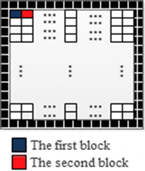
The location of the first and the second blocks
-
Step 3
Other blocks will be scanned to specify the expandable ones. If a block is an expandable one, the watermark bits will be embedded in it:
-
Step 3.1
The AC coefficient will be predicted using the DC values of a \( 3\times 3 \) neighbor block. To do so, a linear estimator is used:
$$ predicted\_ coef{f}_{AC} = {\displaystyle \sum_{i=1}^8}{\tau}_i\times coef{f_{DC}}_i. $$(22)where the coefficients \( {\tau}_i \) are the prediction coefficients and \( {coeff_{DC}}_i \) are the DC coefficients of \( 3\times 3 \) neighbor blocks. For example, in Fig. 2 the AC coefficients of Block are predicted by the DC coefficients of its \( 3\times 3 \) neighbor blocks (i.e. \( {Block}_1 \) to \( {Block}_8 \)) and the coefficients \( {\tau}_i \). The prediction coefficients (\( {\tau}_i \)) are computed by training Adaline neural network. Further information will be given in section 5.1.2.
-
Step 3.2
In this step, the error between the original and the predicted AC coefficient is calculated, as the following:
$$ error= coef{f}_{AC} - predicted\_ coef{f}_{AC}. $$(23)where coeff AC and predicted_coeff AC are the original and the predicted AC coefficient, respectively.
-
Step 3.3
If the AC coefficient is the detection coefficient, a bit ‘1’ will be embedded in the expanded error. If not, the watermark bit will be embedded in it. For embedding a bit of payload in the expanded error, binary representation of the error is computed. Then it is shifted left by one bit to create an empty LSB, into which the bit of payload is embedded.
$$ error = {b}_{l-1}{b}_{l-2} \dots {b}_0. $$(24)$$ watermarked\_ error={b}_{l-1}{b}_{l-2} \dots {b}_0w=2\times error+w. $$(25)where b 0 is the LSB and l is the bit length of error. watermarked_error is the expanded error and w is the bit of payload.
-
Step 3.4
The predicted AC coefficient and the expanded error are added to compute the watermarked AC coefficient.
$$ watermarked\_ coef{f}_{AC}= predicted\_ coef{f}_{AC}+ watermarked\_ error. $$(26)
-
Step 3.1
-
Step 4
If a block is a non-expandable one, the watermark bit will not be embedded in it. In this case, a bit ‘0’ is embedded in the expanded error of the detection coefficient by the proposed algorithm.
-
Step 5
For transferring to spatial domain, the inverse reversible Hadamard transform is applied to blocks. In order to create the watermarked image, the \( 4\times 4 \) blocks are attached together.

The pseudo code of the watermark embedding algorithm is shown in the Fig. 5.

The pseudo code of the embedding phase
5.1.2 The prediction coefficients determination
As mentioned in the embedding phase, the AC coefficients are predicted by the linear function (22). The prediction coefficients in this function are important for more accurate predicting. These coefficients can be a constant number. However, selecting the constant value decreases the visual quality. Since, one value is used to predict all AC coefficients.
If the AC coefficients are predicted accurately, the error values between the original and the predicted coefficients will be lower. Therefore, the quality of the watermarked image will be higher. For more accurate prediction, the coefficients \( {\tau}_i \) are calculated by Adaline neural network.
Adaline uses the image local information, AC and DC coefficients, to compute coefficients \( {\tau}_i \). Desired outputs of Adaline neural network (or d in Eq. (13)) are the original AC coefficients of all blocks which were located in previous rows of current block. The inputs of the Adaline neural network (or I in Eq. (13)) are the corresponding DC coefficients of \( 3\times 3 \) neighbor blocks of those were located in previous rows. Therefore, the Eq. (13) changed as follows:
By the above equation, we do not need the training phase to tune the weights of the neural network (or τ). So, weights can be computed by the linear Eq. (27) directly and the complexity will be critically decreased. This equation is computed for the whole blocks which are in the same row not for every single block separately. Then the computed coefficients will be used to predict the AC coefficients.
Figure 6 illustrates this strategy. The prediction coefficients of blocks which were located in the second row are calculated by their DC coefficients of \( 3\times 3 \) neighbor blocks and the AC coefficients of blocks in the first row. The prediction coefficients of blocks which were located in the third row are computed using the AC coefficients of blocks in the first and the second rows and their DC coefficients of \( 3\times 3 \) neighbor blocks. For computing the prediction coefficients of blocks in the fourth row, the AC coefficients of blocks in the first, the second, the third rows; and their DC coefficients of \( 3\times 3 \) neighbor blocks are used. This strategy is repeated till the end. Note that, since the first and the last rows are marginal ones, no watermark is embedded in the so-called blocks.

The procedure of the prediction coefficients
In the extraction phase, we have the same strategy. Since the blocks located in the previous rows are recovered earlier, we can use them to compute the prediction coefficients after the extraction of the bits of payload. (i.e. The blocks of the first row are the marginal ones and they are used to compute the prediction coefficients of the blocks which were located in the second row. After extraction the watermark bits and recovery the original AC coefficients from the blocks of the second row, blocks which were located in the first and second row are used to calculate the prediction coefficients of blocks in the third row and so on).
5.2 Watermark extraction and image restoration phase
In this phase, the watermark is extracted from the watermarked image in the transform domain. Then the host image will be recovered exactly. First, the watermarked image is divided into \( 4\times 4 \) non-overlapping blocks. Then the reversible Hadamard transform is applied to each block. The length of the watermark is extracted from the first and the second blocks. The detection coefficient of other blocks is checked, afterward. If the extracted payload bit of the detection coefficient is ‘1’, this block will be considered as a watermarked block. But if the extracted payload bit is ‘0’, the block won’t have any watermark bit. To extract a bit of payload, the AC coefficient is predicted. Then the watermarked error is computed and the bit of payload is extracted from it. The pseudo code of the watermark extraction algorithm is illustrated in the Fig. 7. We explain this algorithm extensively through the following steps:

The pseudo code of the extraction phase
-
Step 1
The watermarked image is divided into \( 4\times 4 \) non-overlapping blocks. Each block is commuted to transform domain by the reversible Hadamard transform.
-
Step 2
The length of the watermark is extracted from the first and the second blocks by the proposed algorithm.
-
Step 3
According to the extracted length, other blocks are scanned. In each block, the embedded bit of payload (the detection bit) is extracted from the detection coefficient by the proposed algorithm.
-
Step 3.1
If the detection bit is ‘0’, there won’t be any watermark bit in the block.
-
Step 3.2
If the detection bit is ‘1’, the watermark bits will be extracted based on the following steps:
-
Step 3.2.1
The AC coefficient is predicted by the so-called predictor function in Eq. (22).
-
Step 3.2.2
The watermarked error between the watermarked and the estimated AC coefficient is computed.
-
Step 3.2.3
In this step, the payload bit is extracted from the expanded error, as the following:
$$ w= watermarked\_ error-2\left\lfloor \frac{watermarked\_ error}{2}\right\rfloor . $$(28)Then the original error is calculated:
$$ error=\left\lfloor \frac{watermarked\_ error}{2}\right\rfloor . $$(29) -
Step 3.2.4
To recover the original AC coefficient, the payload bit and the original error are subtracted from the watermarked AC coefficient.
$$ coef{f}_{AC}= watermarked\_ coef{f}_{AC}- error-w. $$(30)
-
Step 3.2.1
-
Step 3.1
-
Step 4
Blocks are commuted to spatial domain using the inverse of the reversible Hadamard transform. Then the \( 4\times 4 \) blocks are attached together to recover the original image.
6 Experimental results
This section presents the performance analysis of the proposed method. The study was done over commonly used standard images and military ones with size \( 512\times 512 \) pixels. They are depicted in Fig. 8.

Test set: 512 × 512 grayscale images (a) Baboon (b) Barbara (c) Boat (d) F_16 (e) Lena (f) Village and the military images: (g) to (l) are Militay1 to Military6, respectively
At the beginning, we would rather explain some terms. The watermark is a random string bit. The embedding capacity or payload size is measured by counting the number of embedded payload bits per pixel. Peak Signal-to-Noise Ratio (PSNR) is used to evaluate the performance of the proposed method.
where MSE is the mean squared error between the watermarked and the original images, that it is defined as follows:
where X, \( {X}^{\prime } \) are the original image and the watermarked image with size \( M\times N \), respectively.
Figures 9 and 10 show the result of applying the proposed method to “Lena”, and “Military1” with different payloads.

The original and watermarked grayscale images (a) Original image “Lena” (b) 42.27 dB with 0.5 bpp (b) 35.76 dB with 0.84 bpp (c) 33.30 dB with 0.95 bpp

The original and watermarked grayscale images (a)Original image “Military1”,(b)45.54 dB with 0.3 bpp(c)43.35 dB with 0.5 bpp(d)41.65 dB with 0.8 bpp
The simulation results for the proposed method are shown in Fig. 11. In this figure, Column (d) shows the difference between the host and the restored images. This difference is zero, which proved that the proposed method can recover the original image exactly after extraction.

Image restoration (a) Original image, (b) Watermarked image, (c) Restored image, (d) The difference between (a) and (c), 0.1 bpp
As mentioned in section 3, embedding the bits of payload in the LSB of errors provides a better quality comparing to embedding in the LSB of coefficients; since the difference between the original coefficient and the watermarked one –which is modified by embedding in the expanded error- is less, in comparison to directly embedding. The comparison between these methods is depicted in Table 1. As you see, the results prove this claim. To perform direct embedding the same as Lin’s [23], the AC coefficients are shifted to the left by one bit to create an empty LSB. Then the bits of payload will be embedded in them. In the extraction phase, if the value of the watermarked coefficient is an even number, a bit ‘0’ will be extracted. If not, a bit ‘1’ will be extracted.
6.1 Parameter analysis
In this section, the effects of the different values of Th and τ on the visual quality are discussed. The parameter Th and the parameter τ are analyzed in sections 6.1.1 and 6.1.2, respectively. As noted before, Th is the predefined threshold and τ is the prediction coefficient.
6.1.1 The effect of threshold parameter on the visual quality
As previously mentioned, a predefined threshold is used to detect the smooth blocks. The different values of Th affect the visual quality. Table 2 presents the effect of different Th on PSNR. When no threshold is defined, the bits of payload can be embedded in all blocks. In other words, there is no limitation. In this case, the capacity will increase while the visual quality will critically decrease. Threshold determination improves the quality but reduces the capacity.
6.1.2 The effect of the prediction coefficients on the visual quality
As mentioned in section 5.1.2, the prediction coefficients can be considered as a constant number or can be computed by Adaline. Table 3 illustrates the effect of the prediction coefficients on PSNR. In this table, two constant numbers 0.01 and 0.05 are considered as the prediction coefficients. The Adaline neural network finds better coefficients due to its use of the image local information; while, one value is used to predict all AC coefficients by the constant number. As it shows, the Adaline could provide better quality.
In the embedding phase, the prediction error is calculated between the original and the predicted AC coefficients. The watermark bits are embedded into the AC coefficients based on the prediction error. The prediction error histogram is plotted as shown in Fig. 12. If the predicted coefficient is similar to the original one, then most of the error values will be low and close to zero. For the original AC coefficient, prediction by Adaline has the highest frequency of zero prediction error, followed by the constant numbers. Since Adaline predicts the AC coefficients accurately, the error values between the main and the predicted coefficients will be lower.

Prediction error histogram for the AC coefficients. a Lena b Military1
6.2 Image authentication analysis
Content authentication has been analyzed by different types of attacks and image processing operations. In Fig. 13, after embedding the bits of payload, an object was removed from the watermarked image. Afterward the original image was restored from the tampered watermarked image. The difference between the original and the restored image are computed. It is obvious that the so-called difference will be zero in the case of the non-tampered watermarked image. Cell (d) shows the location of manipulation.

Image authentication, a Original image, b Watermarked image, c Tampered watermarked image, d The difference between the original and the extraction image
In Fig. 14, Column (a) displays the watermarked images, Column (b) illustrates the tampered ones, Column (c) shows the difference between the original and the extracted payload for non-tampered watermarked images, and Column (d) is the difference between the original and the extracted payload for tampered ones. Column (d) is not black completely, which means that the watermarked image is not authentic. In first row of Fig. 14, an object has been added to “Lena” image. In second row, “Baboon” has been resized 0.5 times. In third row, “Village” image has been 90° rotated. In the fourth row, JPEG compression with quality factor 75 has been applied to “F_16” image. In row five, salt and pepper noise has been added in “Military1” image. In the last row, Gaussian noise with zero mean and 0.01 variance has been added in “Military4” image.

Image Authentication, a Watermarked image, b Tampered watermarked image, c The difference between the original and the extracted payload for non-tampered image, d the difference between the original and the extracted payload for tampered image
6.3 Comparison result
We compare the proposed method with Tian’s [33], Celik’s [8], Thodi’s [32], Kim’s [20], Lin’s [23], Mahmoudi’s [6], and Al_Qershi’s [1]. Tian’s, Celik’s, and Thodi’s are the basic methods in the reversible watermarking while Lin’s, Mahmoudi’s, Al_Qershi’s, and Kim’s are newly proposed schemes. As mentioned in section 2, Tian’s, AL_Qershi’s, and Lin’s methods are some of transform domain ones. Thodi’s and Mahmoudi’s schemes are prediction based. Kim’s method is histogram based. Celik’s method uses the CALIC compression algorithm.
In Table 4, the proposed method has been compared to some basic schemes (i.e. Tian’s, Celik’s, and Thodi’s). As it shows, six sample images are selected for comparison. The proposed method provides the highest performance in all capacities. But the proposed method cannot achieve to a high capacity in highly textured images, like “Baboon”, when the value of Th equals to 15.
Figure 15 presents the comparative results of the embedding capacity versus the distortion (in PSNR) on “Lena”, “F_16”, and “Baboon”, respectively. In this figure, the proposed method has been compared to some recent schemes (i.e. Lin’s, Mahmoudi’s, Al_Qershi’s, and Kim’s methods). In this comparison, the value of Th equals to 15. As you see, the results of Lin’s, Mahmoudi’s, and Kim’s are close to each other. In “Lena” image the quality of the proposed method is higher than the compared ones. The proposed method outperforms Lin’s, Mahmoudi’s, and Al_Qershi’s in “F_16” image, but if the capacity is between 0.1 and 0.2 bpp, the quality of Kim’s method is higher than the proposed one. In the highly textured images like “Baboon”, the proposed method leads to a higher quality. But, it cannot provide a high capacity. As mentioned in section 6.1.1, using a threshold enhances the visual quality but reduces the capacity. Therefore, threshold determination in the proposed method decreases the embedding capacity.

Comparison results of embedding capacity in bpp versus distortion in PSNR with some existing reversible schemes (a) Lena (b) F_16 (c) Baboon, Th = 15
7 Conclusion
In this paper a new reversible watermarking method in Hadamard domain is proposed. AC coefficients are predicted by a linear predictor function. The coefficients of the predictor function are determined using an Adaline neural network for predicting accurately. In the proposed method, for the first time, the reversible Hadanmard transform is used to commute the original image. Based on our experimental results, the reversible Hadamard transform gives the better result in comparison to others, like DCT and integer DCT. In this method, the watermark is embedded in the expanded error instead of embedding in the expanded coefficients. Thus, the quality of the watermarked image will increase. As mentioned before, transform domain schemes provide the higher complexity in comparison to spatial domain methods. Therefore, the proposed method leads to more complexity than spatial domain schemes. To evaluate the performance of the proposed method a comparative study with some well-known reversible watermarking methods is given. The obtained results confirm the superiority of the proposed method in comparison to the studied ones.
References
Al-Qershi OM, Khoo BE (2013) Two-dimensional difference expansion (2D-DE) scheme with a characteristics-based threshold. Signal Process 93(1):154–162
An L, Gao X, Li X, Tao D, Cheng D, Li J (2012) Robust reversible watermarking via clustering and enhanced pixel-wise masking. IEEE Trans Image Process 21(8):3598–3611
An L, Gao X, Yuan Y, Tao D, Cheng D, Ji F (2012) Content-adaptive reliable robust lossless data embedding. Neurocomputing 79:1–11
An L, Gao X, Yuan Y, Tao D (2012) Robust lossless data hiding using clustering and statistical quantity histogram. Neurocomputing 77:1–11
Arsalan M, Malik SA, Khan A (2012) Intelligent reversible watermarking in integer wavelet domain for medical images. J Syst Softw 85:883–894
Aznaveh AM, Torkamani-Azarn F, Mansouri A, Kurugollu F (2010) Reversible watermarking using statistical information. EURASIP J Adv Signal Process 2010, 738972. doi:10.1155/2010/738972
Barton JM (1997) Method and apparatus for embedding authentication information within digital data. U S Patent 5646:997
Celik MU, Sharma G, Tekalp AM, Saber E (2005) Lossless generalized LSB data embedding. IEEE Trans Image Process 14(2):253–266
Chan YK, Chen WT, Yu SS, Ho YA, Tsai CS, Chu YP (2009) A HDWT-based reversible data hiding method. J Syst Softw 82:411–421
Chang CC, Pai PY, Yeh CM, Chan YK (2010) A high payload frequency-based reversible image hiding method. Inf Sci 180:2286–2298
Coltuc D, Chassery JM (2007) Very fast watermarking by reversible contrast mapping. IEEE Sig Process Lett 14(4):255–258
De Vleeschouwer C, Delaigle JF, Macq B (2003) Circular interpretation of bijective transformations in lossless watermarking for media asset management. IEEE Trans Multimedia 5:97–105
Du Y, Zhang T (2009) A reversible and fragile watermarking algorithm based on DCT, Proceeding of the IEEE International Conference on Artificial Intelligence and Computational Intelligence, 301–304
Feng JB, Lin IC, Tsai CS, Chu YP (2006) Reversible watermarking: current status and key issues. Int J Netw Secur 2(3):161–171
Gao X, An L, Li X, Tao D (2009) Reversibility improved lossless data hiding. Signal Process 89:2053–2065
Gao X, An L, Yuan Y, Tao D, Li X (2011) Lossless data embedding using generalized statistical quantity histogram. IEEE Trans Circuits Syst Video Technol 21(8):1061–1070
Gao L, Gao T, Sheng G, Cao Y, Fan L (2012) A new reversible watermarking scheme based on integer DCT for medical images, Proceeding of the IEEE International Conference on Wavelet Analysis and Pattern Recognition, 33–37
Iliyaeu AM, Le PQ, Dong F, Hirota K (2012) Watermarking and authentication of quantum images based on restricted geometric transforms. Inf Sci 186:126–149
Kamran AK, Malik SA (2014) A high capacity reversible watermarking approach for authenticating images: exploiting down-sampling, histogram processing, and block selection. Inf Sci 256:162–183
Kim KS, Lee MJ, Lee HY, Lee HK (2009) Reversible data hiding exploiting spatial correlation between sub-sampled images. Pattern Recogn 42:3083–3096
Lei B, Tan E-L, Chen S, Dong N, Wang T, Lei H (2014) Reversible watermarking scheme for medical image based on differential evolution. Expert Syst Appl 41:3178–3188
Li C, Yang R, Liu Z, Li J, Guo Z (2016) Semi-fragile self-recoverable watermarking scheme for face image protection. Comput Electr Eng 1–10. doi:10.1016/j.compeleceng.2016.01.026
Lin Y-K (2012) High capacity reversible data hiding scheme based upon discrete cosine transformation. J Syst Softw 85:2395–2404
Lin CC, Tai WL, Chang CC (2008) Multilevel reversible data hiding based on histogram modification of difference images. Pattern Recogn 41:3582–3591
Lou DC, Chou CL, Tso HK, Chiu CC (2012) Active steganalysis for histogram-shifting based reversible data hiding. Opt Commun 285:2510–2518
Mao Q, Li F, Chang C-C (2015) Reversible data hiding with oriented and minimized distortions using cascading trellis coding. Inf Sci 317:170–180
Narawade N, Kanphade R (2011) Reversible watermarking: a complete review. Int J Comput Sci Telecom 2:46–50
Ni Z, Shi YQ, Ansari N, Su W (2006) Reversible data hiding. IEEE Trans Circuits Syst Video Technol 16(3):354–362
Sachnev V, Kim HJ, Nam J, Suresh S, Shi YQ (2009) Reversible watermarking algorithm using sorting and prediction. IEEE Trans Circuits Syst Video Technol 19(7):989–999
Sarukhanyan H, Agaian S, Egiazarian K, Astola J (2007) Reversible Hadamard transform. Facta Univ (NIS) 20(3):309–330
Saryazdi S, Nezamabadi-pour H (2005) A blind digital watermark in hadamard domain. World Acad Sci Eng Technol 3:126–129
Thodi DM, Rodriguez JJ (2004) Reversible watermarking by prediction-error expansion, Image Analysis and Interpretation, 6th IEEE Southwest Symposium on, 21–25
Tian J (2003) Reversible data embedding using a difference expansion. IEEE Trans Circ Syst Video Technol 13(8):890–896
Tsai H-M, Chang L-W (2010) Secure reversible visible image watermarking with authentication. Signal Process Image Commun 25:10–17
Wang N, Men C (2012) Reversible fragile watermarking for 2-D vector map authentication with localization. Comput Aided Des 44:320–330
Widrow B, Hoff ME Jr (1960) Adaptive switching circuits. IRE WESCON Convention Record, 96–104
Wu X (1997) Lossless compression of continuous-tone images via context selection, quantization, and modeling. IEEE Trans Image Process 6(5):656–664
Wu X, Liang X, Liu H, Huang J, Qiu G (2006) Reversible semi-fragile image authentication using zernike moments and integer Wavelete transform, Digital Rights Management. Technologies, Issues, Challenges and systems. LNCS in Computer Science 3919:135–145
Yang CY, Hu WC, Lin CH (2010) Reversible data hiding by coefficient-bias algorithm. J Inf Hiding Multimed Signal Process 1(2):91–100
Zhao Z, Luo H, Lu ZM, Pan JS (2011) Reversible data hiding based on multilevel histogram modification and sequential recovery. Int J Electron Commun 65:814–826
Author information
Authors and Affiliations
Corresponding author
Rights and permissions
About this article

Cite this article
Pakdaman, Z., Saryazdi, S. & Nezamabadi-pour, H. A prediction based reversible image watermarking in Hadamard domain. Multimed Tools Appl 76, 8517–8545 (2017). https://doi.org/10.1007/s11042-016-3490-3
Received:
Revised:
Accepted:
Published:
Issue Date:
DOI: https://doi.org/10.1007/s11042-016-3490-3