
Abstract
3D shape retrieval may find the existing models as reference for design reuse. 3D segmentation decomposes models into new elements with large granularity and salient shapes to replace the faces in a solid model. In this way, it may reduce the complexity of a CAD model and make a local salient shape more prominent. Therefore, a retrieval method for 3D CAD solid models based on region segmentation is proposed in this paper. To deal with the problems of poor efficiency and uncertain results, a three-step segmentation method for CAD solid models is introduced. First, face adjacency graph (FAG) descriptions for query models and data models are created from their B-rep models. Second, the FAGs are segmented into a set of convex, concave and planar regions, and the relations among the regions are represented with a region graph. Finally, the sub-graphs are combined recursively to form optimal region sub-graphs with respect to an objective function through an optimal procedure. To avoid using complex graph matching or sub-graph matching for model shape comparison, region property codes are introduced to represent face regions in a CAD model. The similarity between the two compared models is evaluated by comparing their region property codes. The experiments show that the proposed method supports 3D CAD solid model retrieval.
1 Introduction
The popularity of 3D modeling tools in industries has generated a large amount of 3D CAD solid models. As the number of 3D models is increasing rapidly and some 3D models can be obtained from public and proprietary databases, how to reuse the existing 3D models as well as the knowledge of design have become significant for creating new designs. As 3D retrieval can help users discover the desired models, it has soon become an active topic in the academic community.
Most existing retrieval approaches for 3D models focus on mesh models instead of solid models. However, 3D solid models are more likely to be reused in manufacturing industry. Constructive solid geometry (CSG) and boundary representation (B-rep) are two popular descriptions for 3D solid models. CSG (formerly called computational binary solid geometry) is a technique used in solid modeling. The technique allows a modeler to create a complex surface or object by combining objects with Boolean operators. B-rep is an approach in solid modeling for representing shapes by using the limits. A solid is represented as a collection of connected surface elements, the boundary between solid and non-solid. As the standard for the exchange of product model data (STEP) provides a mechanism to present and exchange data in the life cycle of a product, different B-rep models are easily exchanged with STEP. And CSG description of a 3D solid model is non-unique, B-rep is usually used to represent and analyze solid models [12, 18]. Furthermore, face adjacency graphs (FAGs) can be easily created from B-rep models and the existing graph or sub-graph matching can be used for shape comparisons of 3D models. FAG is an ordered pair G f = (V f , E f ), where V f is a set of the vertices that describes the model faces with their properties, and E f is a set of the edges that describes the model edges with their properties. Therefore, some retrieval approaches for 3D solid models based on FAGs have been proposed [10, 12, 24, 36, 38].
However, hundreds of faces are observed in an actual complex model and the granularity of the faces (such as polygonal planes and cylindrical faces) in a complex model is not large enough, which produces a FAG with a larger size and a higher degree of complexity. One way to resolve this problem is to segment 3D solid models into a set of face regions with large granularity to replace the faces in a CAD model. After 3D models are decomposed into a set of face regions, another task for 3D shape retrieval is the shape matching among face regions. Here, region property codes are introduced to represent face regions in a CAD model. As CAD models are mainly composed of regular geometry faces (such as plane, cylinder, cone and sphere) and the topologies of mechanical part models are determined by the types of their adjacency faces, the face property and region property descriptions for CAD models become feasible. Moreover, the region property codes are easy to create, and the code comparison is faster than the model shape comparison by sub-graph matching. Then the similarity between two compared models is evaluated by calculating the similarity of their region property codes. Although 3D segmentation usually incurs a heavy overhead cost, it is indispensable for 3D shape retrieval because it can obviously reduce the complexity of a CAD model by increasing the granularity of the model elements, and the extracted face regions usually contain some semantic information for efficient model comparisons.
The rest of this paper is organized as follows. First, literature reviews and the related terminology definitions are addressed in Sections 2 and 3. Then, region segmentation for 3D solid models is presented in Section 4. In Section 5, the similarity evaluation of 3D models based on the comparison of region property codes is introduced in detail. Following this section, some results of experiments based on the proposed approach are given in Section 6. Finally, the paper presents some conclusions in Section 7.
2 Literature reviews
2.1 3D model retrieval
Shape comparison is essential in the operation of 3D retrieval. Because the direct comparison between two 3D models is impractical, shape descriptors originated in 3D models are usually used for the purpose of comparison. Recently, 3D shape descriptors have been researched widely in the computer graphics area. Most of 3D descriptors can be categorized as histogram-based approach, transform-based approach, view-based approach, and graph-based approach, and the combinations of the above approaches. Shape distributions are typically histogram-based methods, which evaluate the similarity for 3D models by comparing their probable distributions. The sampled distributions are the distances between two points or angles between normal vectors of two points on the model face [29]. Spherical harmonics [20] and 3D Zernike [28] are typical transform-based descriptors for 3D shape comparison, which have rotation, translation and scaling invariance. View-based approaches are derived from the idea that the two models should be similar if they are similar in different directions. Then, 2D projections of 3D models in various directions [11, 17] are adopted to describe 3D models. Compared with 3D descriptors, the level of the complexity of 2D projections is low. Graph-based approaches include Skeleton graphs [5], Reeb graphs [4], feature graphs [3] and FAGs [10, 12, 24, 36, 38]. These methods have an advantage that they can be used for exact shape matching. However, they usually require intricate graph matching algorithms.
Most of above-mentioned methods only support global shape retrieval instead of partial shape retrieval. However, partial retrieval may be used more frequently in engineering. In recent years, partial retrieval of 3D models has become an active topic in the academic community, and several approaches have been proposed. Most of the proposed approaches use model segmentation [14, 26], local feature extraction [2, 3], bag of segments [6, 19] or salient features [16], and the shape descriptors are generated in the same way as the global models [5, 21]. More related literatures of partial retrieval can be found in [22, 32]. For partial retrieval of 3D models, the features identified in models dynamically determine which local structures will be matched in a matching process. Although this is a reasonable approach for retrieval purposes, the number of matching operations may be huge for retrieval from a large library.
For 3D model retrieval, some researchers have specialized in CAD models [9]. El-Mehalawi et al. [12] retrieved CAD models based on FAGs, whose nodes correspond to model faces (such as plane, cylinder, sphere or spline face). Tao et al. [36] introduced FAGs to describe CAD models for 3D shape retrieval. Saber et al. [30] adopted feature point graph (FPG) to represent 2D shapes of a CAD model. The advantage of FAGs and FPGs is that they are easy to create, but their sizes may be too large for a CAD model. Cardone et al. [8] have developed a retrieval approach for CAD models based on the similarity of machining process. Li et al. [21] used feature dependency directed acyclic graph to represent and decompose CAD models for reusable model retrieval. The decomposed components of a CAD model can capture some related engineering knowledge as well as their shapes. Similar to [12] and [36], a FAG is adopted to represent a 3D CAD model in this paper. As the granularity of the faces in a CAD model is not large enough, model segmentation is introduced to reduce its complexity.
2.2 Model segmentation
3D mesh segmentation provides the applications for the fields like reverse engineering, medical imaging, etc. Compared with 3D mesh segmentation, there is still some work to do for 3D solid segmentation. Since most of literatures related to 3D mesh segmentation have been reviewed in [1, 27, 34], we only focus on solid model segmentation in this paper.
The existing approaches for 3D solid model segmentation mostly focus on machining feature recognition. Shah et al. [33] proposed a half-space approach to partition a solid model into a set of maximum convex volumes. However, half-space partitioning for a solid model with curved faces is impracticable in some scenarios. Analogously, Buchele et al. [7] developed an approach to divide solid model into the combination of the half-spaces. But their method is difficult to practice when handling non-describable quadric objects missing the additional information. Sakurai et al. [31] developed a technology to decompose a curved object into maximal volumes with the half-spaces. But if the number of the cells is huge, the efficiency of decomposition may be very poor. Woo et al. [37] tried to increase the scalability of the maximal volume partition through recursively bisecting solid models and combining bisected volumes. Lu et al. [23] developed a technology based on CLoop to automatically divide a solid model into hex meshable volumes. The characteristic of CLoop is that the edges in a CLoop have the same concave and convex [15]. As there are many types of CLoop, its identification is an intractable task. Ma et al. [25] divided solid models along with Cutting Loops. In their study, the volumes are derived from face shells, which are determined by selected cutting loops. Bespalov et al. [3] proposed a Scale-Space feature extraction technique to divide polyhedral faces of a 3D solid model into face patches. This technique can be applied to matching and retrieval of solid models. In their work, the variations of face curvatures were used to extract salient shape features. The salient shape feature is a face region which has variations of face curvatures with its surrounding areas.
Inspired by [3], we propose a retrieval approach for 3D CAD solid models based on region segmentation in this paper. In our work, a different way is adopted to segment solid models into face regions with large granularity and salient shape. Based on our researches, we find that some 3D solid models (such as mechanical parts) have obvious boundaries between their faces, and model segmentation based on curvature criterion usually produces inappropriate segmentation results. Region growing and clustering algorithm are two popular technologies for model segmentation. The former may get various segmentation results when different seed faces are selected for starting growing. The latter may produce a certain result when the optimization process has traversed all possible combinations. Obviously, clustering algorithm has poor efficiency. To deal with the problems of poor efficiency and uncertain results, a three-step segmentation method for 3D solid models is introduced in this paper. The segmentation criterion is that the faces in a region have consistent convexity. First, FAG descriptions for query models and data models are built from their B-rep models. Second, FAGs are segmented into a set of convex, concave and planar regions, and the relationships among the regions are represented with a region graph. Finally, the sub-graphs are combined recursively to form optimal region sub-graphs with respect to an objective function through an optimal procedure.
3 Terminology definitions
A CAD model should be transformed into a FAG before it is segmented. El-Mehalawi et al. proposed an approach for creating a FAG from a STEP file in [12]. Similarly, we use a FAG to express a CAD model in this paper. According to the curvatures, the faces in a CAD model can be classified into convex faces, concave faces, planar faces and saddle faces [35]. In consideration of external edge angle, the edges in a face can be divided into convex edges, concave edges, tangent edges, convex- tangent edges and concave–tangent edges [13]. Before introducing region segmentation for a CAD model, some terminology definitions are firstly given in the following.
Definition 1
If FAGs G i = (V i , E i ) and G = (V, E) satisfy the following conditions:
we define G i as G’s Induced Graph (IG).
Definition 2
For a face region, if its faces are all planar while their interior edges are all tangent, we define it as a Planar Region (PR).
Definition 3
Convex Region (C v R) (Concave Region (C c R)) is a face region whose faces are all convex (concave) or planar while their interior edges are all convex (concave), convex (concave) - tangent or tangent, and it does not belong to a PR.
Based on Definitions 1, 2 and 3, IG can be classified as Planar Region Graph (PRG), Convex Region Graph (C v RG) and Concave Region Graph (C c RG).
Definition 4
The vertices in a FAG G can be categorized as the following three types:
-
The convex (concave) vertex expresses a convex (concave) face or a planar whose edges are all convex (concave) or convex (concave)-tangent in G. Here, we use a symbol ‘+’ (‘-’) to represent it.
-
The hybrid vertex expresses a face whose edges have inconsistent convex (concave) convexity. Here, we use a symbol ‘*’ to represent it.
In Fig. 1a, f 1 is a convex vertex, and f 2 is a concave vertex, but f 3 is a hybrid vertex because f 3 represents a planar with convex edges and concave edges. As some adjacent edges might not exist in a sub-graph of a FAG, a hybrid vertex may be in different forms in different sub-graphs. In Fig. 1b~c, the hybrid vertex v 2 is concave in sub-graph G 1, but convex in sub-graph G 2. Here, the symbols “+”, “-”and “*” denote convex, concave and tangent edge, respectively.

An example of the vertex type. a A CAD solid model and its vertex type. b A FAG G. c G’s sub-graph G 1. d G’s sub-graph G 2
Definition 5
Let G i (i = 1, 2,…, n) be an IG of a FAG G = (V, E), and G i be a PRG, C v RG or C c RG. If G is segmented into a set of IGs
we define S as G’s Face Region Segmentation.
Definition 6
The two IGs G 1 and G 2, can be merged if their vertices have consistent convexity while their edges have consistent convexity on condition that all edges exist.
4 Face region segmentation
4.1 Overview of the proposed segmentation method
To deal with the problem of poor efficiency and uncertain results, a three-step segmentation method for CAD models is proposed. First, FAG descriptions are created from their B-rep models. Then, based on the classification of faces and edges, a FAG is initially segmented into a set of PRG, C v RG and C c RG. Finally, the sub-graphs are recursively combined to form optimal region sub-graphs with respect to an objective function through an optimal procedure. The detailed steps are given in the following.
-
(1)
Recognize the faces with convex or concave convexity;
-
(2)
Recognize the faces with hybrid convexity;
-
(3)
Merge the recognized faces into optimized regions.
Figure 2 gives an example for face region segmentation. As seen from Fig. 2, a FAG G is initially segmented into a set of G’s IGs S i = {G 1, G 2,…, G i ,…, G |S| } while S i is transformed into the optimized result S o by performing an optimization procedure.

Face region segmentation process. a A FAG G. b Initial segmentation result S i. c Optimized result S o
4.2 Initial segmentation
According to Definition 4, the vertices in a FAG have the types of convex, concave and hybrid. Here, we introduce Procedures 1 and 2 to recognize their types. Procedure 1 recognizes the faces that definitely belong to a C v R or C c R while Procedure 2 recognizes the faces with hybrid convexity.
-
Procedure 1. An algorithm for recognizing the faces with convex and concave convexity:
-
Step 1
Delete hybrid vertices ‘*’ and their adjacency edges in a FAG G;
-
Step 2
Delete ‘-’ edges from ‘+’ vertices and ‘+’ edges from ‘-’ vertices;
-
Step 3
Recognize the maximum adjacency sub-graph set S + = {G +1 , G +2 , …, G + i , …, G + p } with ‘+’ vertices and S − = {G −1 , G −2 , …, G − j , …, G − q } with ‘-’ vertices respectively;
-
Step 4
Check whether each G + i or G − j is G’s IG. If not, remove it from S + or S −;
-
Step 5
If G + i or G − j is single-vertex sub-graph, remove it from S + or S −;
-
Step 6
Return to S + (C v Rs’ set) and S − (C c Rs’ set).
-
Step 1
In Procedure 1, we can find the maximum adjacency sub-graph with ‘+’ vertices and the maximum adjacency sub-graph with ‘-’ vertices. After S + and S − are extracted from G, the remaining sub-graphs are G 1 = G - S +- S −. To identify the maximum adjacency sub-graphs C v RG (Cc RG) in G 1, we transform their ‘*’ vertices into ‘+’ (‘-’) vertices by removing their ‘-’ (‘+’) edges.
-
Procedure 2. An algorithm for recognizing the faces with hybrid convexity:
-
Step 1
Delete each ‘-’ edge of G 1 and regenerate the vertex types for G 1;
-
Step 2
Identify the maximum adjacency sub-graph set S +1 = {G +1,1 , G +1,2 , …, G +1,i , …, G +1,p1 } in G 1, where G +1,i has only ‘+’ vertices and ‘+’ edges;
-
Step 3
Check whether each G +1,i is G’s IG. If not, remove it from S +1 ;
-
Step 4
Restore the edges of G 1 that were removed in Step 1;
-
Step 5
Delete each ‘+’ edge of G 1 and regenerate the vertex types for G 1;
-
Step 6
Identify the maximum adjacency sub-graph set S −1 = {G −1,1 , G −1,2 , …, G −1,j , …, g −1,q1 } in G 1, where G −1,j has ‘-’ vertices and ‘-’ edges only;
-
Step 7
Check whether each G −1,j is G’s IG. If not, remove it from S −1 ;
-
Step 8
If both S +1 and S −1 are empty,
-
Step 8.1.
Each vertex in G 1 generates a single-vertex sub-graph, and adds it to S*;
-
Step 8.2.
Exit the procedure;
-
Step 8.1.
-
Step 9
Add S1 + to S +, S −1 to S −; remove the vertices of S 1 and their edges from G 1; and go to Step 1.
Each iteration in the procedure above can find a maximum adjacency sub-graph C v RG or C c RG.
-
Step 1
4.3 Optimize the initial segmentation
After the initial segmentation, the FAG G is turned into S i = {G 1, G 2,…} = S +∪S −∪S *. The single-vertex sub-graph in S * may be a C v RG, C c RG or PRG, depending on whether it represents a face with convex, concave or planar type. As the sub-graphs in S i may be combined into a better segmentation, sub-graph merging is indispensable.
In Definition 6, a sub-graph G i may have several mergeable adjacency sub-graphs. To ensure that the result of merging is determinate, an optimization objective function is selected for evaluating the average relevance of all faces in a region. The relevance of a face v in a region G i is the number of the edges linking v and its adjacency vertices in a region, which can be formulated as follows:
Then, the average relevance of all faces in a region G i is
where |V i | represents the number of the vertices in V i . If face region segmentation is S = {G 1, G 2,…, G |S| }, the average relevance in all regions has the following form:
where |S| represents the number of the regions in S. Using Eq.(1), we may select the merged region that makes f(S) maximal.
Suppose G 1 and G 2 can be merged. The merging condition for G 1 and G 2 can be formulated as follows:
Here, |V 1 | and |V 2 | are respectively the vertex numbers of G 1 and G 2; and |E| is the number of adjacency edges between G 1 and G 2. Based on Eq.(2), optimization algorithm for initial segmentation can be expressed as follows.
-
Procedure 3. An optimization algorithm for initial segmentation:
-
Step 1
Set S = S i = {G 1, G 2,…} and the merged flag F = False;
-
Step 2
Check each sub-graph pair G i and G j in S.
-
Step 2.1.
If sub-graph pairs satisfy the Eq. (2), merge them and set F = True.
-
Step 2.2.
Check the next sub-graph pair.
-
Step 2.1.
-
Step 3
If F = False, return to S and exit; else, update S = {G 1, G 2,…} and go to Step 2.
-
Step 1
5 Similarity evaluation for CAD models based on region property codes
5.1 The code descriptions for a face region
Here, CAD model retrieval is achieved by comparing the similarity among face regions generated in Section 4. As the code is easy to be created and is convenient for the comparison, we introduce region index code Index to represent region properties of a CAD model and face context code fcontext to represent face properties of a region.
5.1.1 Region index code
Region index code Index represents the convexity of a region and its face types, which can be formulated as follows:
where Rc and Rft are integers that get their values respectively from region convexity and face types, the two region properties mentioned above. Specifically, Rc =0, 1 or 2, if the region is a PR, C v R, or C c R, then Rft has the following form:
where ft i (i = 0 ~ 4) is the integer 1 or 0, and the cases of subscript i = 0 ~ 4 respectively correspond to five face types: plane, cylinder, cone, sphere and others. If there exist faces with the i-th surface type in the region, then ft i = 1; otherwise, ft i = 0.
5.1.2 Face context code in a region
-
(1)
The code descriptions for face properties
Here, we introduce a face code f that represents the properties of a face. Face property code f has the following form:
$$ f=10\times ft+ fc, $$(5)where f, ft and fc are integers, and ft and fc respectively express face types and face convexity. The cases of ft = 0 ~ 4 respectively correspond to plane, cylinder, cone, sphere and others while fc = 0 ~ 3 respectively correspond to planar, convex, concave, and others.
-
(2)
The code descriptions for edge properties
Similarly, a code e is introduced to represent edge properties, and it has the following form:
$$ e={5}^0\times f{t}_{\max }+{5}^1\times f{t}_{\min }+{5}^2\times ec, $$(6)where ft min and ft max are the minimum and maximum values of the codes that express the types of two adjacent faces. The parameter ec represents the edge convexity, which is determined by the dihedral angle β of two incident faces; if β = 180°, ec = 0; β < 180°, ec = 1; β > 180°, ec = 2.
-
(3)
Calculation of face context code
First, a FAG G r = (V r , E r ) is introduced to represent all faces and their adjacency relations in a region. Then, the FAG G r is turned into a layer FAG G rc based on the shortest distance between the vertex v r and its adjacent vertices. In G rc , let the vertex v r itself form the layer L 0, and the vertices in the layer L k (k = 1, 2,…,m) has the shortest distance k from the vertex v r . An example for a layer FAG G rc is given in Fig. 3. It can be seen from Fig. 3, a layer FAG G rc around the vertex v 0 is divided into three layers, the vertex v 0 forms the layer L 0; the vertices v 1,1, v 1,2 and v 1,3 form the layer L 1 while the vertices v 2,1, v 2,2, v 2,3, v 2,4 and v 2,5 form the layer L 2. Finally, a face context code fcontext for each vertex v r in V r is calculated from the adjacent vertices of v r with different distances, which has the following forms:
$$ \begin{array}{l} fcontext(v) = f(v)-{C}_1-{C}_2-\cdots -{C}_{\mathrm{m}},\hfill \\ {}{C}_k=l{o}_k\times {10}^0+{10}^2\times l{i}_k+{10}^4\times f{v}_k,\hfill \\ {}l{o}_k=\left({\displaystyle \sum_{e_i\in {L}_{k-1}\times {L}_k}e\left({e}_i\right)}\right)/\left|{L}_{k-1}\times {L}_k\right|,\hfill \\ {}l{i}_k=\left({\displaystyle \sum_{e_i\in {L}_k\times {L}_k}e\left({e}_i\right)}\right)/\left|{L}_k\times {L}_k\right|,\hfill \\ {}f{v}_k=\left({\displaystyle \sum_{v_i\in {L}_k}f\left({v}_i\right)}\right)/\left|{L}_k\right|.\hfill \end{array} $$(7)Fig. 3 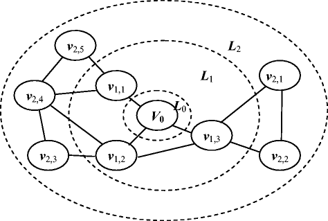
Layers around the vertex v r
In the formulas above, L k-1 × L k is the set of edges between L k-1 and L k , and L k × L k is the set of edges in L k . The parameters f(v i) and e(e i) are respectively calculated in Eqs. (5) and (6).
-
(4)
Statistics of face context codes in a region
To reduce the number of matching operations for the comparison of region shape, all the face context code fcontexts in a face region with the same value should be counted. The statistic results have the following forms:
$$ {n}_1- fcontex{t}_1,\cdots, {n}_k- fcontex{t}_k,\cdots, {n}_m- fcontex{t}_m. $$

In the expression above, fcontext k (k = 1,2,…, m) is the k distinct fcontext codes and n k is the number of faces with code fcontext k in a region.
5.2 Similarity evaluation for face regions
Let Index q be region index codes of query region r q and Index d be region index codes of data region r d , and n qi -fcontext qi (i = 1,2,…, a) and n dj -fcontext dj (j = 1,2,…,b) be their respective face context codes. To evaluate the similarity between r q and r d , fcontext qi and fcontext dj should be decomposed into the following forms:
In the expressions above, m and n are the numbers of FAG layers in regions r q and r d . Let
Then, the similarity s(r q , r d ) between region r q and region r d has the following forms:
In the expression above, s(r q , r d ) = 0 represents that the region r q and region r d are matched.
5.3 Similarity evaluation for CAD models
For a region r qx (x = 1,2,…,u) in a query model M q and a region r dy (y = 1,2,…,v) in a data model M d , let s(r qx , r dy ) be the similarity between r qx and r dy . The similarity s(M q , M d ) between M q and M d is given in Procedure 4.
-
Procedure 4. An algorithm for calculating s(M q , M d )
-
Step 1
Initialize s(M q , M d ) = 0.0; count =0.0; threshold t; input s(r qx , r dy ).
-
Step 2

-
Step 3
If (count ≥ 1.0) s(M q , M d ) = 1/(1+ s(M q , M d )/u);
else s(M q , M d ) = 0.0.
-
Step 4
Output s(M q , M d ).
In Procedure 4, s(M q , M d ) = 1.0 denotes that the query model M q and data model M d are matched. From Section 5.2, we know that there are few similarities between r qx and r dy if s(r qx , r dy ) is large. Therefore, a larger threshold t may find more data models as reference for inspirational purposes while a smaller threshold t may discover fewer models that are similar to a query model in all aspects.
-
Step 1

6 Experimental results
Here, some experimental results for 3D model segmentation and model retrieval are presented. The experiments are conducted on a computer with 3.0 GHz CPU and 1.0 GB RAM, and two model databases. The first library is downloaded from http://www.designrepository.org/datasets/functional.tar.bz2, which is used for evaluating 3D model segmentation, precision and recall measure. The second library is self-created, which includes 450 feature-rich 3D models. Most of them are downloaded from National Design Repository and Purdue Engineering Shape Benchmark, and are used for evaluating retrieval efficiency and its effect.
6.1 3D solid model segmentation
First, some 3D solid models are also introduced to examine the segmented effect. In Fig. 4, we can see that the proposed segmentation method is feasible and most of surface regions have certain engineering semantics. Then, four 3D CAD solid models in Fig. 4 of [3] are selected for evaluating the quality of model segmentation. For the purpose of comparison, the initial segmentation result S i, the optimized result S o and the decomposed results in Fig. 4 of [3] are listed together in Table 1, and each face region is set in a different color. From Table 1, it can be seen that the face regions in the initial segmentation result S i and the optimized result S are more reasonable and their local geometric features are more prominent. Finally, an efficiency curve for the proposed segmentation approach is given in Fig. 5. From this curve, we can find that the time for segmenting a 3D solid model with 500 surfaces is shorter than 1.5 s. Because there are tens or even hundreds of faces in a 3D solid model, the efficiency of the proposed segmentation approach may satisfy the demand of practical application.

Surface segmentation results for some 3D solid models (each surface region is set in a different color)

Efficiency curve for 3D solid model segmentation
6.2 3D model retrieval based on the similarity of face regions
First, three typical models with rich features are chosen for evaluating retrieval effect and efficiency in the second database. The experimental results are listed in Table 2. It can be seen from Table 2 that local structures with yellow color in retrieved models have 4, 9 and 6 faces, and their similar local structures with red color are found in the library. The figures of each returned model shown below indicate the matching similarity. Since the calculation of region codes were conducted at the offline stage, the retrieval time given in Table 2 does not include the time required for the calculation of the codes. Moreover, the retrieval time shown in Table 2 is the average time of 30 runs of the same retrieval. The experimental results show that the proposed approach is feasible, and that it is promising for satisfying the demand of engineering applications.
Then, we introduce a precision and recall measure to evaluate retrieval effect. For the purpose of comparison, the precision-recall graph is plotted together with Fig. 9 of [36] and Fig. 10 of [3], and they are listed in Fig. 6. In Fig. 6, plot 1 is for Reeb graph method, plot 2 is for Scale-Space method with the max-angle distance function and simple sub-graph isomorphism for matching, plot 3 is for the original Scale–Space method with a geodesic distance function, plot 4 is for a random retrieval method, and plot 5 is for sub-graph matching based on gradient flows in Lie group, while plots 6(threshold t = 0.05) and 7 (threshold t = 0.2) are for our proposed approach. Compared with plots 1 ~ 4, the plot 6(threshold t = 0.05) has an advantage in precision measure while the plot 7(threshold t = 0.2) has a merit in recall measure. Compared with plot 5, the plot 7(threshold t = 0.2) has a merit in recall measure. Partial retrieval of CAD models in [36] is an exact retrieval method, which supports users to find data models similar to a query model in all aspects. For the proposed method, different thresholds t can be adopted to meet various requirements. A larger threshold t may find more data models that have a certain similarity to a query model while a smaller threshold t may discover fewer models that are similar to a query model in all aspects. When users are not sure what are their desired reusable models and only aim at getting inspiration from retrieved models, they may prefer to use a larger threshold t.

7 Conclusions
We propose a retrieval method for 3D CAD solid models based on region segmentation in this paper. Here, we use FAGs to represent 3D CAD solid models. The FAG descriptions have a merit that they are easy to be created from B-rep models and the existing graph matching or sub-graph matching algorithms can be used for model comparison. But the size of a FAG for a complex model may be large, which brings about sub-graph matching with poor efficiency because of its NP problem. In this paper, 3D solid models are segmented into a set of PRs, C v Rs and C c Rs, which remarkably reduces the complexity of a CAD model. The face region descriptions for a CAD model capture some related engineering semantics as well as their shapes, which can be applied to 3D shape retrieval.
The significant contributions of our work lie in that an approach of region segmentation is adopted to reduce the complexity of a CAD model while the region property codes are introduced to represent face regions. For 3D shape retrieval, most unrelated data models can be filtered by comparing their region index code Index, which can markedly improve the retrieval efficiency. Besides, a face context code fcontext which considers the characteristics of neighbor faces in a region brings code descriptions with excellent shape resolution.
References
Agathos A, Pratikakis I, Perantonis S et al (2007) 3D mesh segmentation methodologies for CAD applications. Comput-Aided Des Appl 4(6):827–841
Bai J, Gao S, Tang W et al (2010) Design reuse oriented partial retrieval of CAD models. Comput Aided Des 42(12):1069–1084
Bespalov D, Regli W, Shokoufandeha A (2006) Local feature extraction and matching partial objects. Comput Aided Des 38(9):1020–1037
Biasotti S, Giorgi D, Spagnuolo M et al (2006) Sub-part correspondence by structural descriptors of 3D shapes. Comput Aided Des 38(9):1002–1019
Biasotti S, Giorgi D, Spagnuolo M et al (2008) Size functions for comparing 3D models. Pattern Recogn 41(9):2855–2873
Bronstein AM, Bronstein MM, Guibas LJ, Ovsjanikov M (2011) Shape Google: geometric words and expressions for invariant shape retrieval. ACM Trans Graph 30(1):1.1–1.22
Buchele SF, Crawford RH (2004) Three-dimensional halfspace constructive solid geometry tree construction from implicit boundary representations. Comput Aided Des 36(11):1063–1073
Cardone A, Gupta SK, Deshmukh A, Karnik M (2006) Machining feature-based similarity assessment algorithms for prismatic machined parts. Comput Aided Des 38(9):954–972
Cardone A, Gupta SK, Karnik M (2003) A survey of shape similarity assessment algorithms for product design and manufacturing applications. J Comput Formation Sci Eng 3(2):109–118
Chu CH, Hsu YC (2006) Similarity assessment of 3D mechanical components for design reuse. Robot Comput Integr Manuf 22(4):332–341
Daras P, Axenopoulos A (2010) A 3D shape retrieval framework supporting multimodal queries. Int J Comput Vis 89:229–247
El-Mehalawi M, Allen MR (2003) A database system of mechanical components based on geometric and topological similarity, Part I: representation. Comput Aided Des 35(1):95–105
Fu MW, Ong SK, Lu WF et al (2003) An approach to identify design and manufacturing features from a data exchanged part model. Comput Aided Des 35(11):979–993
Funkhouser T, Kazhdan M, Shilane P et al (2004) Modeling by example. ACM Trans Graph 23(3):649–660
Gadh R, Prinz FB (1992) Recognition of geometric forms using the differential depth filter. Comput Aided Des 24(11):583–598
Gal R, Cohen-Or D (2006) Salient geometric features for partial shape matching and similarity. ACM Trans Graph 25(1):130–150
Gao Y, Dai Q, Zhang N (2010) 3D model comparison using spatial structure circular descriptor. Pattern Recogn 43(3):1142–1151
Gao S, Shah JJ (1998) Automatic recognition of interacting machining features based on minimal condition sub-graph. Comput Aided Des 30(9):727–739
Jing W, Peng W (2014) Intrinsic local features for 3D CAD retrieval using bag-of-features. J Comput Inf Syst 10(11):4511–4518
Kazhdan M, Funkhouser T, Rusinkiewicz S (2003) Rotation invariant spherical harmonic representation of 3D shape descriptors. In: Proceedings of the Eurographics Symposium on Geometry Processing
Li M, Zhang YF, Fuh JYH et al (2009) Toward effective mechanical design reuse: CAD model retrieval based on general and partial shapes. ASME J Mech Des 131(12):121501.1–121501.8
Liu ZB, Bu SH, Zhou K et al (2013) A survey on partial retrieval of 3D shapes. J Comput Sci Technol 28(5):836–851
Lu Y, Gadh R, Tautges TJ (2001) Feature based hex meshing methodology: feature recognition and volume decomposition. Comput Aided Des 33(3):221–232
Ma L, Huang Z, Wang Y (2010) Automatic discovery of common design structures in CAD models. Comput Graph 34(5):545–555
Ma LJ, Huang ZD, Wu QS (2009) Extracting common design patterns from a set of solid models. Comput Aided Des 41(12):952–970
Misher F, Hanrahan P (2010) Context-based search for 3D models. ACM Trans Graph 29(6):182.1–182.10
Misic M, Stojcetovic B (2014) 3D mesh segmentation for CAD applications. Center for Quality
Novotni M, Klein R (2004) Shape retrieval using 3D Zernike descriptors. Comput Aided Des 36(11):1047–1062
Osada R, Funkhouser T, Chazelle B, Dobkin D (2002) Shape distributions. ACM Trans Graph 21(4):807–832
Saber E, Xu Y, Tekalp AM (2005) Partial shape recognition by sub-matrix matching for partial matching guided image labeling. Pattern Recogn 38(10):1560–1573
Sakurai H, Dave P (1996) Volume decomposition and feature recognition, Part II: curved objects. Comput Aided Des 28(6–7):519–537
Savelonas MA, Pratikakis I, Sfikas K (2014) An overview of partial 3D object retrieval methodologies. Multimed Tools Appl. doi:10.1007/s11042-014-2267-9
Shah J, Shen Y, Shirur A (1994) Determination of machining volumes from extensible sets of design features. In: Shah J, Mantyla M, Nau D (eds) Adavances in feature based manufacturing. pp. 129–157
Shamir A (2008) A survey on mesh segmentation techniques. Comput Graphics Forum 27(6):1539–1556
Sonthi R, Kun jur G, Gad HR (1997) Shape feature determination using the curvature region representation. Proceedings of the 4th Symposium on Solid Modeling and Applications Atlanta. pp. 285–296
Tao SQ, Huang ZD, Zuo BQ et al (2012) Partial retrieval of CAD models based on the gradient flows in Lie group. Pattern Recogn 45(4):1721–1738
Woo Y, Sakurai H (2002) Recognition of maximal features by volume decomposition. Comput Aided Des 34(3):195–207
Zhang J, Xu Z, Li Y et al (2013) Generic face adjacency graph for automatic common design structure discovery in assembly models. Comput Aided Des 45(8):1138–1151
Acknowledgments
This work is supported in part by the National Natural Science Foundation of China (No.51275182) and the Provincial Key Technologies R & D Program of Qinghai (Grants: 2011-G-A5A).
Author information
Authors and Affiliations
Corresponding author
Rights and permissions
About this article

Cite this article
Tao, S., Wang, S. & Chen, A. 3D CAD solid model retrieval based on region segmentation. Multimed Tools Appl 76, 103–121 (2017). https://doi.org/10.1007/s11042-015-3033-3
Received:
Revised:
Accepted:
Published:
Issue Date:
DOI: https://doi.org/10.1007/s11042-015-3033-3