
Abstract
Depth-image-based rendering (DIBR) has become an important technology in 3D displaying with its great advantages. As a result, more and more 3D products copyright problems turn out. Since either the center view with depth image or the synthesized virtual views could be illegally distributed, we need to protect not only the center views but also the synthesized virtual views. In this paper, a robust watermarking method for DIBR 3D images is proposed. After applying three-level DWT to the center image, we utilize spread spectrum technology to embed the watermark into suitable coefficients of the sub-blocks of the center image, by this way we make our method robust to typical signal distortions, such as JPEG compression, noise addition and median filter. Meanwhile, in order to make the proposed method robust to some common geometric distortion attacks, SIFT-based feature points are used for geometric rectification to eliminate the effect caused by geometric distortion attacks. As the experimental results shown, the proposed method is much more robust to the common signal distortion attacks with lower BER (bit error rate) compared with existing methods. With geometric rectification, our method also performs good robustness to some simple affine transformations. In addition, the proposed watermarking method also has good robustness to the common operations of DIBR processing system.
1 Introduction
Now the key technology of 3D video is focusing on virtual viewpoint rendering. Model -based Rendering (MBR) and Image-based Rendering (IBR) are the types of traditional virtual viewpoint rendering method. MBR is applicable only to a single object 3D modeling [3]. The performance of IBR is determined by the interpolation algorithm. In other word, in order to get 3D images with high quality, we need a large number of viewpoints for sampling, so the amount of video data is unbearable. Moreover, the video acquisition device and digital communication network existing are unable to meet the need of IBR [9, 16]. There is another 3D representation technology different from MBR and IBR, which is named depth-image-based Rendering (DIBR) [8]. In DIBR system, according to the depth information of the pixel in center image, the pixel can be directly transformed to a new pixel in a new image plane of another viewpoint, and we can generate the virtual left and right images by computing the depth information about each pixel. As a result, it is very easy to transmit and store the DIBR 3D images (including the center image and depth image) because the depth image is a grayscale image with limited size. Therefore we can easily achieve the 3D video effects with little additional information.
The natural advantages of DIBR in representation of 3D video will greatly promote the development of 3D industry, making the 3D products spreading rapidly. However, with the rapid development of this technology, a variety of problems about the 3D product copyright protection should be solved.
There have been some watermarking schemes proposed to protect the 2D images, some of which can resist the signal and geometric distortion attacks [1, 2, 5, 6, 19, 26, 28]. However, the virtual images and center image should be protected by embedding watermark in the center image, which is different from the 2D images. As shown in Fig. 1, both of the depth image and the center image will be transmitted to the content viewer, who can perform DIBR operation to generate the virtual left and right images. Unfortunately, in the content consumer side where the depth image may not be distributed, either of the center image or generated virtual images could be illegally distributed. If one of these images is illegally distributed, the depth image may not be available for watermark extraction. Moreover, additional noise could be introduced by DIBR rendering process. Taking into account the particular characteristics of DIBR 3D images, some watermarking methods have been proposed to deal with the problems mentioned above. In [10, 12], watermarking schemes for DIBR 3D images and stereo images are proposed. However, the watermarking extraction procedure of these schemes needs the participation of the original image or the watermarked image without any distortion. For these reasons, some improved methods have been proposed. In [15], a watermarking scheme for 3D video focusing on perceptual embedding was proposed, which is robust against lossy compression and adding Gaussian noise. In [18], Lin and Wu proposed watermarking algorithm by embedding three watermarks into the DCT domain of the center image. Considering the estimated relationship between the center image and the virtual images generated from the center image with corresponding depth image, the three watermarks embedding should be performed with a suitable order. In this scheme the watermark can be successfully extracted with a low bit error rate from the center image or the virtual images with any extraction order. The simulation results show that the watermarking method proposed by Lin and Wu can be robust against some common signal distortion attacks, such as JPEG compression and noise addition. However, this scheme could not be robust to geometric distortion attacks. In Kim’s paper [13], DT-CWT was exploited to develop a watermarking algorithm for 3D images in a DIBR system, where the embedded watermarks are extracted blindly. The simulation results showed that the watermarking method proposed by Kim is robust to not only general signal and geometric distortion attacks, but also some special types of attacks generated in DIBR process such as depth image pre-processing and baseline distance adjusting.

Illegal content re-distribution in the content viewer side
In this paper, we propose a watermarking method for DIBR 3D images, watermark embedded in the center image can be blindly extracted from center image or virtual synthesized images with fixed baseline distance without the participation of the original image when the watermarked images are not attacked by any geometric distortions. Meanwhile, SIFT-based feature points are used to perform geometric rectification, so as to extract watermark from images with geometric distortion attacks. The experimental results show that the proposed watermarking algorithm has good robustness to common signal distortions with lower BER than methods proposed by Lin [18] and Kim [13]. For some common geometric distortion attacks, because of the instability of the adopted geometric rectification method, the robustness to geometric distortions is not good as to the signal distortion attacks. However, the BER is still low within an acceptable range.
This paper is organized as follows. Section 2 briefly reviews the basic DIBR operations. Scale invariant feature transform and spread spectrum are introduced In Section 3, In Section 3, the proposed watermarking scheme based on improved spread spectrum and geometric rectification are also given. Experimental results of the proposed method are demonstrated in Section 4. Conclusions of this work are given in Section 5.
2 A brief overview of DIBR operations
The principle of binocular vision is to obtain the parallax which is related to the depth information of objects. The other way round, we can also generate the virtual views from center views by 3D warping with the depth information of objects. DIBR operations are consisted of pre-processing of the depth image, 3D image warping and hole-filling.
2.1 Pre-processing of depth image
Depth image is an 8-bit grayscale image [8], the video processing uses YUV (Luma and Chroma) space to represent a frame generally. As shown in Fig. 2, (a) is a common 2D image; (b) is the corresponding depth image. Although we can generate the virtual views from center view with the depth image corresponding, there will be some holes appeared in the generated virtual views without any operation to the depth image. So in order to reduce the number of holes and improve the quality of the new images, some pre-processing of depth image should be performed before 3D warping [7, 27].

(a) Center image of Moebius and (b) depth image of Moebius
2.2 3D image warping
Liang Zhang and Wa James Tam [27] proposed a method in their paper, by which we can use the depth information to compute the disparity and generate the virtual views from center view. As shown in Fig. 3, we can find a point P in space, where Z represents the depth value of the point in center view, f is the focal length, C l and C r represents the virtual left viewpoint and virtual right viewpoint respectively. t x represents the value of the baseline distance between C l and C r . We can conclude formula (1) with the geometric relationships as shown in Fig. 3. d represents the value of disparity between the left and right virtual views. Without loss of generality, the value of f is set to 1.

The relationship of pixel in left view, center view and right view
In order to compute the depth value of pixel in center view, the gray values are normalized to two main depth clipping planes, the near clipping plane Z near with gray level 255 and the far clipping plane Z far with gray level 0. According to formula (2), we can compute the depth value Z(v) of P, v represents the gray level value.
2.3 Hole-filling
In fact, some pixels without any information will appear after 3D wrapping, we call these pixels holes. It is because that some new pixels appeared in the virtual image are occluded by the foreground object center image [27]. As shown in Fig. 4, we can find there are some holes in the right virtual view. In order to improve the quality of virtual views, some methods are proposed to fill the holes. In this paper, we adopt linear interpolation as the hole-filling method the same as Kim and Lin.

(a) The center image (b) the right virtual image with holes and (c) the hole-filled image by using linear interpolation
3 Proposed watermarking method
In this section we introduce the proposed watermarking algorithm. We use three-level DWT and linear approximation of the improved spread spectrum (ISS) [18, 21] technique to implement the watermark embedding. In the watermark extraction procedure we compute the correlation between wavelet coefficients of every sub-block and the spread spectrum code to estimate the watermark. In fact, the watermarking extraction procedure doses not need geometric rectification for images without any geometric distortion attacks as shown in Fig. 5a. In order to make the proposed method more robust to some common geometric distortion attacks, we need to rectify the distorted watermarked image before watermark extraction. Figure 5b illustrates the procedure of watermarking extraction with geometric rectification for images with some geometric distortion attacks. The proposed geometric rectification method is illustrated in Section 3.3.

(a) Watermarking extraction without geometric rectification and (b) watermarking extraction with geometric rectification
3.1 Watermark embedding procedure
As shown in Fig. 6, according to the 3D image warping formula (1), we find that there are some differences between the center image and the rendered virtual images; the disparity involved in the rendered virtual images is proportional to the baseline distance t x [27]. So we decide to embed the message into the common parts of the center image and rendered virtual images.

Relationship between the center image and the rendered virtual images
As shown in Fig. 7, the proposed watermark embedding method can be divided into the following steps

Proposed watermark embedding procedure
-
Finding the common parts of the center image and rendered virtual images: Suppose I is a center image with M × N pixels, and p(x i , y j ) is a pixel in I, and we can find the common parts I common as the following formula
In order to make the watermark embedded in I common can be almost fully extracted from virtual images without being affected by pixel horizontal shifting, we set \( {D}_r={D}_l= \max \left(\frac{t_x}{2}\times \frac{f}{Z(v)}\right) \), where \( Z(v)={Z}_{far}+v\times \frac{Z_{near}-{Z}_{far}}{255} \). In the experiment, baseline distance and focal length are set to 5 % of width of the center image and 1. Corresponding to the most varying scenario for the rendering operations Z far is also set to 5 % of width of the center image and Z near = 1 [13, 18].
-
Dividing the common parts of the center image into sub-blocks with 64 × 64 pixels and applying the Three-level DWT to every sub-block: According to S.Mallat’s algorithm, the image can be decomposed into four sub-graphs, size of which is quarter of the original image: horizontal, vertical and diagonal direction of the high frequency detail sub-graphs and a low frequency approximation sub-graph. With the subsequent decomposition, the sub-graph can be decomposed into a smaller sub-graph with the next level resolution by the same way, finally, the image can be decomposed multiple sub-graphs with different directions and different resolution levels. Figure 8 illustrates the result of three-level DWT applied to a image, LL n is a low frequency component, HL n is the high frequency component of the horizontal direction, LH n is the high frequency component of the vertical direction, HH n is the high frequency component of the diagonal direction, n = 1, 2, 3. In the DWT domain, the low frequency component is the best approximation sub-graph of the original image, whose statistical characteristics is similar to original image. High frequency component represents information about the edge and the texture of the image.
Fig. 8 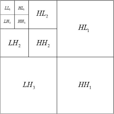
Three-level DWT
-
Scramble watermark message: In order to enhance the security of the embedded message, we use a secret key to scramble the binary image to watermark sequence.
-
Choose the coefficients of suitable sub-band to complete the watermark embedding: It is generally believed that the human eye is less sensitive to noise and distortion in horizontal and vertical direction of the high frequency band. Low frequency part has greater influence on image quality, of which the noise and distortion are much easier to detect. The high frequency part of image is not only with good performance of imperceptibility, but also represents the detail of image. In this paper, we will embed the watermark into the coefficients of LH 3 and HL 3.
-
Improved spread spectrum (ISS) embedding: Suppose H = (h 1, h 2, …, h l ) represents the coefficients about LH 3 and HL 3 of one sub-block, P = (p 1, p 2, … p l ) represents the spread spectrum factor for one bit b of watermark scrambled, α adjusts the signal strength of the inserted bit b, λ indicates the reduction ratio of the interference of H ', we can use the ISS to reduce the interference from H while embedding as following

Where N represents the noise introduced by some operations and H ' represents the interference generated by H computed as
< H, P > represents the inner product between coefficients H of sub-block and P which can be defined as
-
Applying the Inverse three-level DWT to every sub-block to get the watermarked image.
3.2 Watermark extraction procedure
As shown in Fig. 9, the proposed watermark extraction method can be divided into the following steps:

Proposed watermark extraction procedure
-
The same as the embedding procedure, we firstly find I common (common parts) of the watermarked image I watermarked , then we divide I common into 64 × 64 sub-blocks, with every sub-block three-level DWT applied.
Because the depth value of each pixel in center image is different, we need to set D l and D r to a fixed value to extract the watermark from virtual images successfully. As shown in Fig. 10, the disparity changes a little when the intensity of pixel arranges from 0 to 200, so we set \( \begin{array}{cc}\hfill {D}_r={D}_l=\frac{t_x}{2}\times \frac{f}{Z(v)}\hfill & \hfill v\in \left[150,200\right]\hfill \end{array} \), when the baseline t x is set to 5 % of the center image width.

Disparity of pixel with different intensity value in depth map when t x is 5 % of the center image width
-
Compute the correlation between the selected coefficients and the spread spectrum code: In proposed method, we calculate the correlation between the selected coefficients and the spread spectrum code to estimate the extracted watermark.
H represents the coefficients of one sub-block of original image, S represents the coefficients of sub-block with one bit watermark, P represents the pseudo random sequence. Before the watermark extraction we make one assumption as following: the pseudo random sequence P and the noise introduced N are statistically uncorrelated. Therefore we can use the following formula to compute the correlation between P an S. cor(S, P) represents the correlation between P and S, • represents the general inner product:
Where the extracted message b ' can be expressed as b ' = sign(cor(S, P)), and we determine the value of b ' by judging cor(S, P) is a positive or a negative one as following:
-
Scrambling the extracted message to get the watermark.
In fact, we could not know I watermarked is center image watermarked or virtual images watermarked, so we can extract watermark three times according to formula (6), and compute the similarity between the watermark extracted and the original watermark to get the real watermark with the biggest similarity.
3.3 Geometric rectification procedure
In order to make the watermark extraction still accurately when the watermarked image is under some geometric attacks, we use the feature points extracted by SIFT to realize the geometric rectification of image attacked. By this way, we can make the proposed watermarking method with good robustness to geometric attacks.
3.3.1 Detection and matching of feature points
SIFT (Scale Invariant Feature Transform) was proposed by Lowe in 1994 [20]. SIFT is a kind of algorithm extracting the local feature of images based on scale space theory. SIFT seeks the extreme value point in the scale space to extract location, scale and rotation invariant and has proved to be invariant to image rotation, scaling, translation, partial illumination changes, and projective transformations. Furthermore, SIFT also has a certain robustness to changing of view, compression, filtering and adding of noise. We can detect and match the feature points with following steps
-
Select the stable feature points by using the difference of Gaussian (DOG) function to detect Scale-space extrema
Where \( G\left(x,y,\sigma \right)=\frac{1}{2\pi {\sigma}^2}{e}^{-\left({x}^2+{y}^2\right)/2{\sigma}^2} \), L(x, y, σ) represents the scale space of an image I(x, y), k represents the multiple between adjacent scale spaces. In order to search for the Scale-space extrema, the candidate should be compared with its eight neighbors with the same scale and the nine neighbors in the closest scale.
-
Locate each of key-points, then remove the points with low contrast and poorly localized along edges using the following formula
Where H is a 2 × 2 Hessian matrix, D xx , D xy , D yx and D yy is the second derivative of L(x, y, σ), r is the radio between the largest and the smallest eigen value.
-
Assign the orientation of each key-point based on local image properties.
-
Generate a descriptor which is a 128-deminision vector for each feature point from the local image region.
-
Feature points matching: we can calculate the Euclidean distance between the points of two images according to the descriptor of feature points.
3.3.2 Pre-processing of feature points
In order to make watermarking method robust to common geometric distortion attacks, we need to extract SIFT feature points from the watermarked image, and the feature vectors of feature points are used as the synchronization key to rectify the distorted image. After geometric rectification, we can get a new image nearly the same as the original, from which the watermark can be extracted.
However, SIFT was first put forward for image matching with a large number of extracted feature points. Typically, we can extract more than 1000 feature points from an image with 512 × 512 pixels [14]. For example, the number of the feature points extracted from some images of the test data set can reach up to more than 20,000, although not all of these feature points are suitable for watermark synchronization. Every SIFT feature point has a corresponding scale information, feature points with both large and small scale are easy to disappear when the image is attacked.
Therefore, we should remove the points within the scale space that are either too small or too large from all of the feature points. In this paper, we select these feature points with scale from 4 to 8 [4, 14, 17, 20].
3.3.3 Rotation rectification procedure
For the rotation rectification, we can estimate the rotation degree by calculating the angel of lines between the two pairs of feature points matched.
There will be many groups of value about the estimated rotation degree, some of which are close to the true value. However, there are still some error matching making the estimated rotation degree far away from the real value. By computing the mean value of the data, we make the estimated rotation degree much closer to the true value. Here we use the least square method for data fitting. First of all, remove some of the data far away from the others as far as possible, and compute the mean value of the remaining data.
Suppose the fitting curve is y = kx + b, with the first data fitting for data set X we can get the initial mean value k. Then we can find that most data of X is spread to both sides of k and very close to k, however, some data of X is far away from k. In order to get more accurate estimated degree, we follow the below steps to compute the mean value of X
-
Suppose the new data set X ' = {x 1, x 2, ⋯ x m }, where x i ∈ X, x i ≥ k − Δ − n k and x i ≤ k + Δ − n k, n represents the times of iterative operation, Δ is the parameter of error. Then we need compute the mean value k ' of the new data set X '.
-
Repeat the above operations, we can get k ' as the final estimated value, when |k − k '| ≤ ε; or we can get k ' when |k − k '| > ε and the times of iterative operation is over n.
For the reason that stability of feature points extracted from different images is different, there is some error between images in the test database. As shown in the Table 1, the error and estimated degree are listed for test image “Moebius” rotated by (−10∘, − 8∘, − 6∘, − 4∘, − 2∘, − 1∘, + 1∘, + 2∘, + 4∘, + 6∘, + 8∘, + 10∘).
3.3.4 Scaling rectification procedure
For the scaling rectification, we estimate the scaling multiple by calculating the length ratio of lines between any two points. The test image “Moebius” is scaled by (50 %, 75 %, 90 %, 110 %, 150 %) as shown in the Table 2. The result shows the difference between the real scaling multiple and the estimated multiple (Table 3).
3.3.5 Cropping after rotation rectification procedure
We can utilize the method proposed in the above section to estimate the rotation degree θ. Notice that we can rotate the distorted image with degree − θ to perform rotation rectification. However, the image with rotation rectification, which has been cropped some parts of the image, is still different from the original watermarked image without any geometric distortion. In order to estimate the part of image cropped, we can use the matched SIFT feature points to calculate the displacement on the abscissa and ordinate, by which we can estimate the size of the original image. By filling the estimated missing area of rectified image with zero-valued pixels, we can get a new image as shown in Fig. 11.

(a) Image with cropped after rotation and (b) image after rectification
3.3.6 Affine rectification procedure
Affine transformation can be implemented by combining a series of atomic transformation, such as: Translation, Scale, Flip, Rotation, and Shear. Either of above transformations can be represented by a 3 × 3 matrixes, of which the last row is (0, 0, 1). We can use this matrix to change point (x, y) to a new point (x ', y ') as the following formula:
When b = c = d = f = 0, a ≠ 0 and e ≠ 0, we call this transformation Scaling; when a = e = 1, c = f = 0, b ≠ 0 and d ≠ 0, we call this transformation Shearing.
For the scaling, transformation can be represented as following:
According to equation set we can find as follows:
For the shearing, transformation can be represented as following:
Similarly, according to equation set we can also find out:
For the transformation combined with more than two kinds of affine transformation is relatively complicated, specific represented as following:
In order to determine the transformation matrix, we need at least two pairs of matching feature points to get the parameters of affine transformation. Through the analysis above we can conclude when the transformation parameters a, b, c, d are all not zero, the transformation is a combination of scaling and shearing, we can also solve transformation parameters by the least squares method:
Where X = (x 1, x 2 ⋯ x n ), Y = (y 1, y 2 ⋯ y n ), X′ = (x ′1 , x ′2 ⋯ x ′ n ), Y′ = (y ′1 , y ′2 ⋯ y ′ n ).
In fact, the image after geometric correction is still different from the original image without any geometric distortions. Therefore, the error of correction can affect the BER of message extracted from watermarked images.
As shown in Fig. 12b, for the rotation correction, when the error of correction is in [0, 0.2], the average BER of message extracted is below 0.13, at which the message extracted can also be clearly distinguished.

(a) BER of the message extracted with different scale rectification error and (b) BER of the message extracted with different rotation rectification error
As shown in Fig. 12a, for scaling distortion correction, when the error of correction is in [0, 0.002], the average BER of message extracted is below 0.1.
With the error of correction reaching greater than 0.002, the average BER rises sharply, when the error rises up to 0.005, the average BER has exceeded 0.3, and we can hardly distinguish what the extracted message is.
4 Experimental results
In this section, we show the experimental results of the proposed watermarking method, and the robustness to various distortions are compared with the methods proposed by Kim and Lin. Especially we employ two different parameter settings for Lin’s method. In Lin’s method *, the block size is set to 16 × 16, for Lin’s method **, the block size is 64 × 64.
As shown in Fig. 13, in order to construct the test images, 12 pairs of center and depth images are obtained from Middlebury Stereo Datasets [11, 22, 23] and Microsoft Research 3D Video Datasets [29], of which the resolutions are ranged from 450 × 375 to 1390 × 1110. The corresponding depth images are gray scale images of 8-bit level.

Image pairs of center and depth images taken form Middlebury Stereo and Microsoft Research 3D Video Datasets: (a) art; (b) books; (c) dolls; (d) moebius; (e) reindeer; (f) laundry; (g) cones; (h) teddy; (i) ballet; (j) orbi; (k) baby; (l) interview
Different from the method programs by Lin [18], the parameters for DIBR are set with some changes. The parameters for the watermark embedding method are λ = 1 and α = 6, by which can eliminate the interference from the original cover and enhance the robustness of the watermarking against the noise.
4.1 Evaluation of watermarking robustness
As we know, robustness is one of the most basic requirements for image watermarking, and the robustness of a watermark can be determined by the watermark strength α. As shown in Fig. 14, the average BER is reducing when we increase the watermark strength. When the watermark strength α is 2, the average BER of center images has reduced to zero, however the average BERs of the virtual images are still about 0.1, which is unacceptable. When we set the watermark strength α = 6, the average BERs of the virtual images are blow 0.01, moreover the average PSNR of center images is above 46 dB as shown in Fig. 15. In this paper, we evaluate our algorithm with fixed block size which is 64 × 64. Accordingly, the reference pattern can be generated by Hadamard matrix as following: for a block with 64 × 64 the length of the reference pattern reference pattern is 128, which is the same as the length of the spread spectrum sequence.

Average BERs of center image, left image and right image with different watermark strength

Average PSNR of center image with different watermark strength
As shown in Fig. 16, without any distortion, we can extract the embedded message from the watermarked center view with zero bit error rates. The messages extracted from the synthesized left and right view are nearly the same as the original watermark message, with lower bit error rate, which is 0.0031. As listed in Table 4, in the proposed method, the BERs of the messages extracted from the left and right virtual views are much lower than the results obtained by the methods proposed by KIM and LIN.

(a) The original embed image, (b) the extracted watermark from watermarked center image, (c) the extracted watermark from rendered watermarked left image, and (d) the extracted watermark from rendered watermarked right image
In order to show the perceptual quality, we use the average PSNR and structure similarity (SSIM) [25] to measure the watermarked center views, then compare the results with that obtained by Kim’s and Lin’s method. As shown in Fig. 17, for test image “Moebius”, there is nearly no obvious difference between the original center view and the watermarked center view with PSNR 46.60 dB. The results are shown in Table 3, the average PSNR measured for the test image set is 45.70 dB, which is more than the results obtained by Kim’s and Lin’s method.

(a) Original image of “Moebius” and (b) the watermarked image of “Moebius”
In the above section, we embed the watermark into the 12 test images with watermarking algorithm proposed in this paper. Without any distortion, we extract the watermark message from the watermarked center views with zero bit error rate, furthermore, the proposed method shows lower BER for the virtual views, and we find that the proposed method with much stronger robustness to the DIBR process than both Kim’s and Lin’s method.
In fact, both of the center image and virtual images could be distributed. When one of them is illegally re-distributed by the content consumer, it can be distorted by the signal and geometric attacks. Therefore, in order to investigate the robustness of the watermarking method proposed in this paper to the distortions caused by the signal and geometric attacks, we attempt to extract the watermark from the virtual right view, of which the average BER of the message extracted without any attack is much higher. Before the extraction, we apply some signal and geometric distortions to the rendered virtual right view. We use Stirmark benchmark tool [24] to generate such distortions as JPEG compression, additive noise, median filtering, scaling, rotation and cropping after rotation.
As shown in Fig. 18, for the JPEG image compression, the average BER of the message extracted by the proposed method is much lower than the other methods proposed by Kim and Lin, When the quality level of JPEG compression level is 15 (for “Moebius”, when the JPEG compression level is 15, the PSNR is 25.16 dB, and PSNR of image is 25.85 dB when the JPEG compression level is 100), the average BER showed by proposed method is even less than 0.1. If the watermark embedded is binary image, the watermark extracted can be still clearly identified, the performance of the proposed method is much better than Kim’s method. For the additive noise, when the noise level is higher than 5 (for “Moebius”, when the level of additive noise is 1, the PSNR is 28.26 dB, and PSNR of image is 13.04 dB when the level of additive noise is 7), the performance of the proposed method is much better than Kim’s method. For the median filtering, the performance is much better than the two other methods with any median filter size.

Average BER for distorted watermarked right virtual images: (a) JPEG compression; (b) additive noise; (c) median filtering; (d) scaling; (e) rotation; and (f) cropping after rotation
In this paper we use the SIFT feature points for geometric correction, although the SIFT algorithm has good robustness to geometric attack, some of the feature points may make miss matching. If some of the SIFT feature points used for geometric correction are not stable, the experimental results will be affected. As shown in Fig. 18, for the scaling, rotation and cropping after rotation, the performance of proposed method is not stable but acceptable.
The effect of signal and geometric distortions on the synthesized virtual right view has been investigated in above sub-section. In order to investigate the robustness of geometric correction method to the distortion caused by affine transformation, we apply eight common affine transforms as following:
As illustrated in Fig. 19, for the affine transform Mat1-Mat4 such as simply vertical or horizontal shearing transformation, the parameters of transformation matrixes can be much more accurately estimated using the geometric correction method. We can extract the watermark at a lower BER with estimated parameters.

Average BER of the proposed method, Kim’s method and Lin’s methods for various affine transforms
For transform combined with scaling and shearing, we also attempt to estimate the parameters of the transform matrix by using the feature points extracted by SIFT. Notice that there are four parameters should be estimated, so the performance of geometric rectification depends on the stability of feature points we used. In fact, the stability of feature points extracted from some images of the test set is not good enough to estimate the transform matrix exactly, so the average BER of message extracted increases with the transform matrix parameters estimated in a large deviation. As shown in Fig. 19, for the geometric distortion combined with scaling and shearing, the average BER of proposed method is slightly higher than Kim’s, but still much less than Lin’s.
As the above sections shown, the virtual views can be generated by the DIBR rendering process with a proper baseline distance t x , t x represents the important parameter baseline distance. Usually the parameter t x is different in DIBR process in order to be suitable for different people’s visual. For this reason that parameter t x used in watermarking embedded is different from the DIBR rendering process, the performance of watermark extraction may be effected.
In Lin’s method, in order to decide where to embed the watermark in the center image, the relationship of pixels between the center image and virtual image should be found with a fixed t x . So the BER will greatly increase when the value of t x used in the watermarking extraction procedure is not the same as the watermarking embedding procedure. The proposed watermarking method in Kim’s paper is designed with the characteristic of approximate shift invariance of the DT-CWT, the method proposed in Kim’s paper depends on the size of the sub-blocks, once t x is more than the size of sub-block, the message extracted will be all wrong. So choosing the suitable size of sub-block for watermark embedding could avoid this problem. In fact, the process of DIBR could be considered as the translation transform. We use the feature points matched to estimate the number of pixels translated and set the value of D r and D l given in (7). As shown in Fig. 20, the proposed method shows lower and almost consistent BER.

Average BER of the proposed method, Kim’s method and Lin’s methods for the various baseline distance ratio
As illustrated in Section II, the depth image can be modified to generate more natural virtual left and right views in the viewer’s DIBR system. For this experiment, asymmetric smoothing was employed [27]. As demonstrated in Table 5, the BER for most of the 12 test images are much lower than Kim’s method in both case of original depth image and blurred one. On the other hand, for some of the 12 test images, the BERs for the case of original depth image and blurred depth image change little.
4.2 Computational time costs
Suppose the size of center image is M × N, which is divided into m × n sub-blocks. The time complexity of three level DWT and watermark embedding for one bit could be computed as \( O\left(\frac{M}{m}\times \frac{N}{n}+\frac{M\times N}{m\times n\times {2}^3}\right) \), so the time complexity of the whole watermark embedding procedure is \( m\times n\times O\left(\frac{M}{m}\times \frac{N}{n}+\frac{M\times N}{m\times n\times {2}^3}\right)\approx O\left(M\times N\right) \). In the same way, the time complexity of watermarking extraction is O(M × N). For SIFT algorithm, we intend to compute the time complexity in four aspects, Scale-space extrema detection, Key-point localization, Orientation assignment and Generation of key-point descriptors. For an image with size of M × N, the Gaussian pyramid is consisted of k octaves, and every octave has s + 2 intervals. So the time complexity of scale-space construction is \( O\left(M\times N+\frac{M}{2}\times \frac{N}{2}+\dots +\frac{M}{2^k}\times \frac{N}{2^k}\right)\approx O\left(M\times N\right) \), and the time complexity of DOG (Difference of Gaussian) construction is \( O\left(s\times M\times N+s\times \frac{M}{2}\times \frac{N}{2}+\dots +s\frac{M}{2^k}\times \frac{N}{2^k}\right)\approx O\left(s\times M\times N\right) \). Suppose there are M ' × N ' key-points, where M ' × N ' ≪ M × N. So the time complexity of Orientation assignment and Generation of key-point descriptors is O(M ' × N '), and the time complexity of SIFT algorithm is O(M × N) + O(s × M × N) + O(M ' × N ') ≈ O(M × N). For feature points matching, we should calculate the Euclidean distance between the points of two images according to the descriptor of feature points, so the time complexity is O((M ' × N ')2). In the proposed method, when should extract feature points from watermarked image after embedding watermark into the center image, so the time complexity of whole watermark embedding procedure is O(M × N). When the watermarked image is attacked by geometric distortion, we should extract feature points and find the matched points, so the time complexity of whole watermark extraction procedure is O(M × N) + O((M ' × N ')2). In fact, computing the time complexity of SIFT by theoretical analysis is difficult, in order to test the computation cost of the proposed and methods proposed by Kim, we test these watermark embedding methods on 12 images in test dataset and watermark extraction methods on 144 rotated images using a computer with Intel Core i5 CPU (2.67 GHz) and 3GB RAM, and the average computational time are listed in Table 6. As shown in Table 6, the computation cost of proposed watermark embedding is 6.0356 s, including the cost for SIFT algorithm. The computation cost of watermark extraction is 12.6944 s, and the extra cost for SIFT algorithm is 12.0131 s.
5 Conclusions
In this paper we proposed a watermarking method for the center views and virtual views synthesized by DIBR rendering process. The watermark can be blindly extracted without the participation of the original image with fixed baseline distance, when the watermarked images are not attacked by any distortion or only attacked by signal distortion. In order to make the proposed watermarking method robust to the common geometric distortion attacks, feature points extracted by SIFT are used as the watermark synchronization key to eliminate the effect caused by geometric distortion attacks. Experimental results show that the proposed watermarking method has good robustness to JPEG compression, adding noise, median filtering and geometric distortion, and visibility of the binary image message extracted is acceptable. Meanwhile, as the experimental results shown, the proposed watermarking algorithm has good robustness to the changing of baseline in DIBR process. However, accuracy of proposed geometric rectification method is restricted by the stability of the feature points extracted from different images. We will gradually improve these problems in the future research.
References
Alghoniemy M, Tewfik A (2004) Geometric invariance in image watermarking. IEEE Trans Image Process 13(2):145–153
Bas P, Chassery J-M, Macq B (2002) Geometrically invariant watermarking using feature points. IEEE Trans Image Process 11(9):1014–1028
Chan SC, Shun HY, Ng KT (2007) Image-based rendering and synthesis. IEEE Signal Process Mag 24:22–33
Deng C and Cao XB (2009) Geometrically robust image watermarking based on SIFT feature regions. Acta Photonica Sinica 1005–1010
Deng C, Gao X, Li X, Tao D (2009) A local Tchebichef moments-based robust image watermarking. Signal Process 89(8):1531–1539
Dugelay J-L, Roche S, Rey C, Doerr G (2006) Still image watermarking robust to local geometric distortions. IEEE Trans Image Process 15(9):2831–2842
Fehn C (2004) Depth-image-based rendering (dibr), compression, and transmission for a new approach on 3d-tv. SPIE Stereoscop Displays Virt Real Syst XI 5291(1):93–104
Fehn C, La Barre E, Pastoor S (2006) Interactive 3-DTV: concepts and key technologies. Proc IEEE 94(3):524–538
Fujii T, Tanimoto M (2002) Free-viewpoint TV system based on ray-space representation. Proc SPIE Three-Dimension TV, Video, Display 4864:175–189
Halici E and Alatan A (2009) Watermarking for depth-image-based rendering. IEEE Int Conf Imag Process (ICIP) 4217–4220
Hirschmüller H and Scharstein D (2007) Evaluation of cost functions for stereo matching. IEEE Conf Comput Vis Patt Recog
Hwang DC, Bae KH, Kim ES (2004) Stereo image watermarking scheme based on discrete wavelet transform and adaptive disparity estimation. Math Data/Imag Coding, Compress, Encrypt VI, Applications 5208(1):196–205
Kim HD, Lee JW, Oh TW, and Lee HK (2012) Robust DT-CWT water- marking for DIBR 3D images. IEEE Trans Broadcast 58(4)
Lee HY, Kim HS, Lee HK (2006) Robust image watermarking using local invariant features. Opt Eng 45(3):1–11
Lee MJ, Lee JW, and Lee HK (2011) Perceptual watermarking for 3D stereoscopic video using depth information. Int Conf Intell Inform Hiding Multimed Sign Process (IIHM- SP) 81–84
Levoy M and Hanrahan P (1996) Light field rendering. Proc SIGGRAPH- '96 31–42
Li LD, Guo BL, and Pa JS (2008) Feature-based image watermarking resisting geometric attacks. Innov Comput Inform Contrl (ICICIC)
Lin YH, Wu JL (2011) A digital blind watermarking for depth-image-based rendering 3D images. IEEE Trans Broadcast 57(2):602–611
Loukhaoukha K, Chouinard JY, Tsai MH (2011) Optimal image watermarking algorithm based on LWT-SVD via multi-objective ant colony optimization. J Inform Hiding Multimed Sign Process 2(4):303–319
Lowe DG (2004) Distinctive image features from scale-invariant keypoints. Int J Comput Vis 60(2):91–110
Malvar H, Florencio D (2003) Improved spread spectrum: a new modulation technique for robust watermarking. IEEE Trans Signal Process 51(4):898–905
Scharstein D and Pal C (2007) Learning conditional random fields for stereo. IEEE Conf Comput Vis Patt Recog 1–8
Scharstein D, Szeliski R (2003) High-accuracy stereo depth maps using structured light. IEEE Comput Soc Conf Comput Vis Patt Recog 1:195–202
Stirmark Benchmark 4.0 May 2004 [Online]. Available: http://www.petitcolas.net/fabien/watermarking/stirmark/
Wang Z, Bovik AC, Sheikh HR, Simoncelli EP (2007) Image quality assessment: from error visibility to structural similarity. IEEE Trans Image Process 13(4):600–612
Xiang S, Kim HJ, Huang J (2008) Invariant image watermarking based on statistical features in the low-frequency domain. IEEE Trans Circ Syst Video Technol 18(6):777–790
Zhang L, Tam W (2005) Stereoscopic image generation based on depth images for 3d TV. IEEE Trans Broadcast 51(2):191–199
Zheng D, Wang S, and Zhao J (2009) RST invariant image watermarking algorithm with mathematical modeling and analysis of the watermarking process. IEEE Trans Image Process 18(5)
Zitnick C, Kang SB, Uyttendaele M, Winder S, Szeliski R (2004) High -quality video view interpolation using a layered representation. ACM Trans 1111 Graph 23(3):600–608
Author information
Authors and Affiliations
Corresponding author
Appendix
Appendix
Algorithm 1: Watermark embedding
Find common parts in center image using formula (2): img[M][N]
\( BS=64\begin{array}{cc}\hfill :\hfill & \hfill \begin{array}{ccc}\hfill size\hfill & \hfill of\hfill & \hfill sub- block\left(64\times 64\right)\hfill \end{array}\hfill \end{array} \)
Watermark: w[⌊M/BS⌋][⌊N/BS⌋]
Hadamard matrix: p[128][128]
k = 1
for i = 1 to [⌊N/BS⌋]
for j = 1 to [⌊N/BS⌋]
if w[i][j] == 1
Watermark_seq[k] = 1
Watermark_seq[k] = − 1
end
end
end
Scramble Watermark_seq[⌊(M/BS)⌋ × ⌊(N/BS)⌋]
num = 1
for i = 1 to M
for j = 1 to N
block = block(i : i + N − 1, j : j + N − 1)
block = 3 − DWT(block)
Choose LH 3 and HL 3 as cof[128]
\( ip=\frac{\left\langle cof,\kern0.2em p\left[num\right]\right\rangle }{\left\langle p\left[num\right],\kern0.2em p\left[num\right]\right\rangle } \)
for k = 1 to 128
cof[k] = cof[k] + (Watermark_seq[num] + 6 × ip) × p[num][k]
end
Change LH 3 and HL 3 with cof[128]
block = 3 − IDWT(block)
j = j + BS
num = num + 1
end
i = i + BS
end
Algorithm 2: Watermark extraction
Watermark: watermark[3]
BS = 64
Hadamard matrix: p[128][128]
for situation[k] in formula (6)
Find common parts in watermarked image using formula (6): img[M][N]
bit_seq[⌊(M/BS)⌋ × ⌊(N/BS)⌋]
for i = 1 to M
for j = 1 to N
block = block(i : i + N − 1, j : j + N − 1)
block = 3 − DWT(block)
Choose LH 3 and HL 3 as cof[128]
\( ip=\frac{\left\langle cof,\kern0.2em p\left[num\right]\right\rangle }{\left\langle p\left[num\right],\kern0.2em p\left[num\right]\right\rangle } \)
if ip > 0
bit_seq[num] = 1
else
bit_seq[num] = − 1
end
j = j + BS
num = num + 1
end
i = i + BS
end
watermark[k]= bit_seq
end
Similarity: NC[3]
for situation[k] in formula (6)
Compute NC[k] between watermark[k] and Watermark_seq
end
Select the watermark with biggest NC between as the final extracted watermark
Rights and permissions
About this article

Cite this article
Cui, C., Wang, S. & Niu, X. A novel watermarking for DIBR 3D images with geometric rectification based on feature points. Multimed Tools Appl 76, 649–677 (2017). https://doi.org/10.1007/s11042-015-3028-0
Received:
Revised:
Accepted:
Published:
Issue Date:
DOI: https://doi.org/10.1007/s11042-015-3028-0