
Abstract
Action recognition has become a very important topic in computer vision with unconstrained video sequences. There are varieties of approaches to feature extraction and video sequences description, which play important roles in action recognition. In this paper, we survey the main representations along dense trajectories and aggregating methods for the videos in the last decade. We mainly discuss the aggregating methods which are bag of words (BOW), fisher vector (FV) and vector of locally aggregated descriptors (VLAD). Furthermore, the newest mean average precision (mAP) obtained from the references is used to discuss different aggregating methods on realistic datasets. And for more intuitive comparison those aggregating methods, we will evaluate them on KTH in the same conditions. Finally, we analyze and compare those papers’ experimental data to summarize the trends. Based on the reviews from several approaches to action recognition, we further make an analysis and discussion on the technical trends in this field.
1 Introduction
Recognizing actions “in the wild” has been an active research topic in computer vision. Here, a video “in the wild” refers to a video captured under uncontrolled conditions from YouTube, movies, etc.. What’s more, recognizing actions in realistic settings has caught great attention of researchers from real-time video surveillance and security monitoring, automatic video indexing, and human-computer interfaces [10, 16, 37, 55]. Meanwhile, the problem of recognizing actions in videos is challenging, and all difficulties associated with object detection and recognition task, such as large intra-class variations, partial occlusions, low resolution, camera motion, view point changes, geometric and photometric variances and cluttered background, may also be encountered in action recognition. Therefore, decomposition and estimate camera motion, which are based on low rank optimization and features match, are used to modify camera motion [51, 57]. In addition, Kim et.al [20] proposed a method to recognize human actions in arbitrary views by developing 4D space-time features. And Ramanathan et.al [40] provided an overview of the existing methods based on their ability to handle these challenges.
There have been a lot of realistic video datasets proposed for action recognition in the past 5 years, such as Hollywood2 [31], UCF YouTube [29], Olympic [35], UCF50 [41], and HMDB51 [23], UCF sports [43], UCF101 [49], etc.. Some key challenges exist in those datasets, like variation in camera viewpoint and motion, the cluttered background, changes in the position, scale, appearances of the actors, and the large intra-class variation, etc.. Some of them are large-scale datasets which is a large video database such as UCF50, UCF101 and HMDB51 [23, 34], and they are very valuable for evaluating the approaches in real-world action recognition dataset with a large number of classes.
In general, action recognition includes three modules, the feature extraction and description module (the feature module), the video description module, and classification module. The input of the video description module is the feature vectors from the feature module and the output of video description module is video-level descriptor (i.e., mid-level representation or video-level vector) which is obtained by clustering. The input of classification module is video-level descriptor which is more discriminative and compact than feature vector (see Fig. 1). In this survey, we concentrate on the recent techniques which are used for recognizing the realistic action recognition that can obtain the state-of-the-art results. Those techniques include feature extraction, clustering methods and their corresponding classification methods. We focus on feature extraction and description which around dense trajectories such as HOG (histogram of oriented gradients), HOF (histograms of optical flow), MBH (motion boundary histogram), etc.. Dense samples are more prospering compared with sparse interest points [54] and its dense features perform is convinced to have a better performance for complex videos [12, 36, 56]. Meanwhile, we also discuss the popular clustering methods which are bag of words (BOW) [27, 53], fisher vector (FV) [2, 39, 51, 63] and vector of locally aggregated descriptors (VLAD) [17–19]. References [6, 24, 27, 54] indicate that BOW was popularly used for action recognition in the past. In addition, Wang [51] evaluated that FV or VLAD can get better performance than BOW for action recognition in realistic videos. Classifier mainly uses χ2 kernel or linear support vector machine (SVM) for different vector-level representations. In the subsection, we will discuss the popular aggregating methods for action recognition with unconstrained videos.

The action recognition pipeline
For the low-level (i.e., features vector or local descriptor), it is very difficult to distinguish the important parts of the representation, and decide which part could be ignored safely. Algorithms which are based on low-level features are not robust enough to complex environment [25, 28] (e.g., cluttered background, camera movements and illumination changes). Therefore, mid-level representation (i.e., video/image-level representation) [3, 5, 11] was proposed in recent years.
Mid-level representation [3, 5, 11, 65, 66] is more compact, flexible, and adaptable than the low-level one. A lot of researchers have been done to figure out the methods to extract the mid-level features. For instance, a novel pooling method of bag of features (BOF) was proposed by Ballas et al. [3] to improve robustness of action recognition. Fathi et al. [11] and zhang et al. [65, 66] extracted mid-level features based on the Adaboost algorithm. Boureau, et al. [5] used the bag-of-word to form mid-level vectors, etc..
Mid-level representation is generally considered to be a suitable classifier input for to reduce computational cost. How to choose different classifiers for various kinds of mid-level vectors? Generally, BOW adopts non-linear SVM which is χ 2 kernel SVM normally. While the FV and VLAD adopt linear SVM. Sometimes, the classification method is designed to be more suitable for the mid-level vector to improve the performance such as [3, 60].
This paper is organized as following: The core techniques of low-level representation around dense trajectories will be briefly discussed in section II. We introduce these different aggregate methods and discuss the newest (i.e., the state-of-the-art) mean average precision (mAP) [3, 8, 32, 33, 51] of datasets for realistic video sequences under these different aggregate methods in section III. The evaluation conditions, datasets and classification methods are listed in section IV, and we also summarize the newest mAP for all kinds of realistic videos with the different aggregating methods and compare different combination, fusion position, and normalization methods with those aggregating methods. We also evaluate the different aggregate methods on KTH dataset for action recognition in this section. Finally, we discuss the technique trends of future researches and conclusions in section V.
In this paper, we denote that because of the polysemous nature of the words, adopting the same terminologies in the research community is an impossible objective to achieve. Such as mid-level representation has the same meaning with video-level descriptor and BOW equals to BOF in this paper.
2 The methods of low-level representation along dense trajectories
In this section, we discuss the key technique of dense trajectories in the low-level in recent years. Dense trajectories were first proposed by Wang et.al [53] which was inspired by dense sampling. Because dense sampling has shown to improve results over sparse interest points for image classification [12, 36]. And for action recognition, dense sampling at regular positions in space and time outperforms state-of-the-art spatio-temporal interest point detectors [54]. In Wang’s paper they extracted four descriptors which are HOG, HOF, MBH and trajectory (for convenience, we call it Dentr), respectively and used early fusion [48] to combine them. Among which, HOG, HOF and MBH are extracted along trajectory not around the interest points such as 3D-SIFT [46], HOG3D [21], etc.. In particular, HOG descriptor characterizes static appearance, while HOF and MBH descriptors capture dynamic motion. What’s more, HOF captures the local motion information and MBH captures the relative motion information. For realistic videos, they are often complemental to each other, which motivate researchers to fuse these descriptors each other to enhance the discriminative power. They evaluated those video descriptions with bag-of-features approach and have obtained a significant improvement over the state of the art on four datasets which are KTH, YouTube, Hollywood2 and UCF sports, respectively.
However, as the information about clutter motions, such as background changes and camera motions were accumulated, this kind of information was not useful and reduces discriminative power. Hence, the dense sampling was convinced to be not efficient. In the view of above problem, Murthy et al. [33] proposed a technique which selected only a few dense trajectories and then generated a new set of trajectories termed ‘ordered trajectories’, and the ordered trajectories were about 50 % of the actual dense trajectories amount in [53]. Cho et al. [8] robustly identified local motions of interest in an unsupervised manner and used a multiple kernel method to improve the action recognition performance. Table 1 calculates an average selection ratio (ASR) of the number of selected local motion descriptors (LMDs) to the number of full motion descriptor (FMDs) obtained from each video [8]. It shows that local motion selection method selects only a small fraction of descriptors. From Table 2, it shows that even though ordered trajectories and LMDs [8, 33] can reduce trajectories, the performance of benchmark datasets have slightly improved.
Ballas et al. [3] introduced a new space-time invariant pooling scheme with dense trajectories to improve the performance. It shows that the pooling method has a better performance than the ‘ordered trajectories’ and LMDs (Table 2).
From Table 2, we can find that dense trajectories can get the best results for different of datasets. However, it is obvious to show that there is still room for the improvement especially in Hollywood2 and HMDB51 which are the real-world actions. What can we do to improve the performance for unconstrained videos? Wang et al. [51] considered the influence of camera motion. They aimed to estimate camera motion and then removed it from dense trajectories. From Table 3, it shows that camera motion has a slightly influence on performance. Improved trajectories obtain a gain of performance of respectively 3, 3 and 2 % for Hollywood2, HMDB51 and UCF50 while Ballas’ scheme has 9 and 5 % increase for UCF50 and HMDB51. It inspires us to explore video-level module that can improve the performance for unconstrained videos.
In the next section, we will discuss different kinds of aggregate methods in video-level module for action recognition in recent years.
3 The techniques of generate video-level vector
How to bridge semantic gap between low-level features and high-level action categories [44] is a key problem in action recognition. Mid-level representation is more compact and efficient than the low-level representation from previous paper [30].
In general, building a mid-level vector from local features can be broken down into two seeps 1) local features coding and 2) local features pooling (see Fig. 2). There are many coding methods for image classification such as super-vector [7, 67, 68], K-means, OMP-M, Triangle coding and soft thresholding, etc. [22] and polling methods are max pooling and average pooling.

The typical data-flow for generates a video-level vector which reference [22]
Mid-level features perform a point-wise transformation of the descriptors into a representation adapted to the task. Boureau et al. [5] used the bag-of-words (BoWs) as the mid-level representation. From low-level presentation to mid-level, it focuses on two types of modules which are coding and pooling. Koniusz et al. [22] reviewed a number of techniques for generating mid-level features, including two variants of soft assignment, locality-constrained linear coding, and sparse coding. The pooling methods are divided into average pooling and max pooling. In [5], it is shown that hard quantization is better than soft quantization, and sparse coding is better than soft quantization; max pooling is always superior to average pooling, especially when using a linear SVM; the intersection kernel SVM performed similarly to or better than the linear SVM.
To our knowledge, BOW was widely used for action recognition in last decades. And FV and VLAD were used for action recognition in the past 2 years [2, 17, 18, 33, 51]. In the past, FV was popular in image categorization [38]. The fisher vector extended the BOW by encoding high-order statistics (first and, optionally, second order). VLAD was first proposed by Jegou et al. [19] for image search.
Tombnes’s blog [15] indicated that mid-level representation was one of the three trends in computer vision research areas by analyzing paper of CVPR 2013. Therefore, mid-level representation (video-level vector) plays an important role in action recognition. In the subsection we will discuss techniques that are used to achieve mid-level representation.
For image or video vector representation, there are three vector aggregation methods frequently used in action recognition which are BOW, FV, VLAD, respectively. All these methods are aimed at aggregating d-dimensional local descriptors into a single vector representation which represents an image or a video (see Fig. 2). We will discuss them in the subsection, respectively.
-
A.
Bag-of-words
BOW is the first widely used method for action recognition [8, 14, 23, 24, 27, 29, 31, 41, 44, 50, 52–54, 59]. The BOW representation is the histogram of the number of video descriptors assigned to each visual word. Therefore, the dimension of video vector is equal to the number of visual words. The visual words usually obtained by k-means clustering. Hence, BOW is a hard assignment (HA) or hard quantization (see Eq. (1)). The quantization error may be propagated to the spatio-temporal context features and may degrade the final recognition performance. For classification, χ 2 kernel SVM is usually used to classify the BOW representation.
For action recognition, BOW’s simplest form employs HA to solve the following optimization problem:
$$ \begin{array}{c}\hfill \alpha ={\displaystyle { \arg \min}_{\overline{\alpha}}}{\displaystyle {\left\Vert X-M\overline{\alpha}\right\Vert}_2^2}\hfill \\ {}\hfill \mathrm{s}.\mathrm{t}.{\displaystyle {\left\Vert \overline{\alpha}\right\Vert}_1}=1,\overline{\alpha}\in {\displaystyle {\left\{0,1\right\}}^K}\hfill \end{array} $$(1)In practice, Eq. (1) means that a dictionary M has been formed by k-means clustering, every descriptor X is assigned to its nearest cluster with activation equal one. The L1-norm constraint \( {\displaystyle {\left\Vert \overline{\alpha}\right\Vert}_1}=1 \) ensures that α is histograms. Since α can take only binary values, the L1-norm also ensures a single non-zero entry per α. Equation (1) shows that BOW has high quantisation error. Hence, there are two soft assignment methods popular used for action recognition which are FV and VLAD.
-
B.
Fisher vector
The Fisher kernel (FK) is a generic framework which combines the benefits of generative and discriminative approaches. Perronnin et al. [39] showed that they can boost the accuracy of the FK for large scale image classification. And fisher vector only needs to use linear SVM whose training cost is O(N)-where N is the number of training images. While non-linear SVMs’ training time are between O(N2) and O(N3). From [53], it is shown that BOW is not suitable for linear SVM. Hence, FV is faster than BOW’s classification. In recent years, FV was used for action recognition [32, 51]. Paper [51]’s results shows that FV has a better performance than BOW. In addition, Murthy et al. [32] proposed a technique that combines ordered trajectories’ [33] FV with improved trajectories’ [51] FV to improve performance.
The FV is an image/video representation obtained by pooling local image/video features. It is frequently used as a global image/video descriptor in visual classification or action recognition.
While the FV can be derived as a special, approximate, and improved case of the general Fisher Kernel framework, it is easy to describe directly. Set v=(X1,…,XN) to be a series of D dimensional features vectors (e.g., HOG, HOF, MBH), which are extracted from an image/video. Set Θ = (μ k , Σ k , Π k : k = 1, …, K) to be the parameters of a Gaussian Mixture Model (GMM) to fit the distribution of descriptors. The GMM associates each vector Xi to a mode k in the mixture with a strength given by the posterior probability:
$$ {\displaystyle {q}_{ik}}=\frac{{\displaystyle {\left({\displaystyle {X}_i}-{\displaystyle {\mu}_k}\right)}^T}{\displaystyle {\varSigma}_k^{-1}}\left({\displaystyle {X}_i}-{\displaystyle {\mu}_k}\right)}{{\displaystyle {\varSigma}_{t=1}^K}{\displaystyle {\left({\displaystyle {X}_i}-{\displaystyle {\mu}_t}\right)}^T}{\displaystyle {\varSigma}_t^{-1}}\left({\displaystyle {X}_i}-{\displaystyle {\mu}_t}\right)} $$For each mode k, consider the mean and covariance deviation vectors
$$ \begin{array}{c}\hfill {\displaystyle {u}_{jk}}=\frac{1}{N\sqrt{{\displaystyle {\varPi}_k}}}{\displaystyle \sum_{i=1}^N{\displaystyle {q}_{ik}}\frac{{\displaystyle {X}_{ji}}-{\displaystyle {\mu}_{ik}}}{{\displaystyle {\sigma}_i}}}\hfill \\ {}\hfill {\displaystyle {v}_{jk}}=\frac{1}{N\sqrt{{\displaystyle {\varPi}_k}}}{\displaystyle \sum_{i=1}^N{\displaystyle {q}_{ik}}\left[{\displaystyle {\left(\frac{{\displaystyle {X}_{ji}}-{\displaystyle {\mu}_{ik}}}{{\displaystyle {\sigma}_i}}\right)}^2}-1\right]}\hfill \end{array} $$where j = 1,2,…,D spans the vector dimensions. The FV of image/videos V is the stacking of the vectors uk and the vectors vk for each of the K models in the Gaussian mixtures:
$$ \varPhi (V)={\displaystyle {\left[\cdotp \cdotp \cdotp {\displaystyle {u}_k}\cdotp \cdotp \cdotp {\displaystyle {v}_k}\cdotp \cdotp \cdotp \right]}^T} $$where [·]T means the transpose of vector. Hence, each video is represented by a 2DK dimensional FV for each descriptor type.
The FV representation has many advantages w.r.t the BOW. Firstly, it provides a more general way to define a kernel from a generative process of the data: we show that the BOW is a particular case of the FV where the gradient computation is restricted to the mixture weight parameter of the GMM. From paper [32, 51] it is shown that the additional gradients incorporated in the FV bring large improvements in terms of accuracy. Secondly, it can be computed from a much smaller number of centroids in terms of mAP (e.g., a 4000 visual word BOW is comparable to a 256 centroids FV or VALD [9, 17, 33, 51]). Thirdly, even with simple linear classifiers, it can still perform well. A significant benefit of linear classifiers is that they are very efficient to evaluate and computationally economical to learn.
-
C.
Vector of locally aggregated descriptors
VLAD is a simplified non-probabilistic version of FV which is an extremal case of FV. VLAD was first proposed by Jegou et al. [19] for image search. It shows that VLAD achieved a significant outperforms improvement than ever before, and it is more efficient than BOW. In recent years, VLAD was first used for action recognition [17, 33], and it is efficient for its effectiveness compared with a non-linear kernel and post-processed using a component-wise power normalization and L2-normalized (i.e., referred to as SSR), which dramatically improves its performance [17, 33]. Ordered trajectories’ [33] results are 1.9 % (absolute), which is better than paper [17] for HMDB51 dataset.
VLAD is a feature encoding and pooling method, and similar to FV. VLAD encodes a set of local features descriptors V=(V1,…VN) extracted from an image/video using a dictionary built based on clustering method such as GMM or K-means clustering. Set qik to be the strength of the association of data vector xi to cluster μ k , such that and the association may be either soft (e.g., obtained as the posterior probabilities of the μ k are the cluster means, vectors of the same dimension as the data Vi. VLAD encodes feature V by considering the residuals)
$$ {\displaystyle {v}_k}={\displaystyle \sum_{i=1}^N{\displaystyle {q}_{ik}}\left({\displaystyle {V}_i}-{\displaystyle {\mu}_k}\right)} $$The residuals are stacked together to obtain the vector
$$ \varPhi (V)={\displaystyle {\left[\cdotp \cdotp \cdotp {\displaystyle {v}_k}\cdotp \cdotp \cdotp \right]}^T} $$where [·]T means the transpose of vector. Therefore, each video is represented by a DK dimensional VLAD for each descriptor type. There are three normalized methods for VLAD which are component-wise L2 normalization, square-root and L2 normalization, as well as Component-wise mass normalization. Component-wise mass normalization which is called NormalizeMass corresponding to each vector vk is divided by the total mass of features. Square-rooting and L2-normalization [39] which is called SSR corresponding to each Φ(V) := sign(Φ(V))|Φ(V)|α and \( \varPhi (V):=\frac{\varPhi (V)}{{\displaystyle {\left\Vert \varPhi (V)\right\Vert}_2}} \). Component-wise L2 normalization which is called NormalizeComponents [1, 9] corresponding to the vector vk divided by their norm ‖v k ‖2. We will evaluate the three normalized methods in the next section.
In the next section, we will introduce experimental conditions, then discuss and summarize the three aggregating methods, respectively.
4 Analysis and comparison of the experiment data
In this section, we first introduce the datasets, corresponding experimental conditions and classification methods used for action recognition in the references. Then the mean average precision (mAP) is listed for all datasets in the subsection of this paper. In recent years researchers proposed the realistic datasets for research such as Hollywood2 [31], UCF sports [43], Olympic [35], UCF50 [41], HMDB51 [23], UCF101 [49] etc.. UCF50, UCF101 and HMDB51 are large datasets which are more complex compared to Hollywood2. Table 4 shows the list of action datasets.
-
A.
Datasets
KTH [45] composes of 6 classes of 25 human actions. The videos are subject to different zoom rates and have mostly non-cluttered static backgrounds. The evaluation listed in this paper all uses the training/testing division of Schuldt [45].
UCF sports [43] contain ten human actions. The video shows a large intra-class variability. Wang et al. [51] and Cho et al. [8] used a leave-one-out setup and test on each original sequence while training on all other sequences together with their flipped versions.
Olympic Sports [35] has 16 sports actions which consist of athletes practicing different sports. All experiments use 649 sequences for training and 134 sequences for test in our paper.
Hollywood2 (HOHA) [31] contains 12 action classes which are collected from 69 different Hollywood movies. It contains 1707 video split into a training set (823 videos) and a test set (884 videos). Training and test videos come from different movies.
UCF101 [49] has 101 action categories which are classified into 25 groups. From which, Clips of 7 groups are used as test samples and the remains for training.
UCF50 [41] has 50 action categories taken from YouTube. For all 50 categories, the videos are split into 25 groups or 5 groups. Wang et al. [16, 52] and Murthy [33] applied the leave-one-group-out cross-validation to 25 groups. While Ballas et al. [3] used 5 folds leave-one-out group-wise cross validation which is listed in Table 2.
HMDB51 [23] is composed of 6849 videos clips divided into 51 action categories. The different actions have large appearance variation. It all adopts the default training and testing splits [23].
-
B.
Classification method
In general, to classify action recognition of BOW histograms under unconstrained videos, it usually uses a non-linear SVM with a multi-channel χ 2 kernel [23, 27, 31, 53], etc.. We use the multi-channel Gaussian kernel defined by:
$$ K\left({\displaystyle {H}_i},{\displaystyle {H}_j}\right)= \exp \left(-{\displaystyle \sum_{c\in C}\frac{1}{{\displaystyle {A}_c}}{\displaystyle {D}_c}\left({\displaystyle {H}_i},{\displaystyle {H}_j}\right)}\right) $$where Hi={hin} and Hj={hjn} are the histograms for channel c and Dc(Hi,Hj) is the χ2 distance defined as
$$ {\displaystyle {D}_c}\left({\displaystyle {H}_i},{\displaystyle {H}_j}\right)=\frac{1}{2}{\displaystyle \sum_{n=1}^V\frac{{\displaystyle {\left({\displaystyle {h}_{in}}-{\displaystyle {h}_{jn}}\right)}^2}}{{\displaystyle {h}_{in}}+{\displaystyle {h}_{jn}}}} $$where V is the vocabulary size. The parameter Ac is the mean value of the distances between all training samples for channel c [64]. While Adaboost with C.45 may be used to classify the histogram of BOW for action recognition [29].
For FV and VLAD, the linear classifier will be used to classify them with the advantage of low cost [17, 32, 39, 51]. In our experiment, C is set to be 100 for linear SVM, which has been shown to obtain good results when validating on a subset of training samples.
For the tables in this paper, we should note that we list the best results obtained from their corresponding papers, and the performance is measured by mAP over all classes.
-
C.
Evaluation of these aggregation methods
From the above paragraphs, it is shown that FV and VLAD have freshly been used for the application of large-scale action recognition since 2013. In the future we have to explore how to make full use of them. From Table 5, it is shown that FV and VLAD work well for large-scale action recognition. What’s more, the FV and VLAD significantly outperform BOW for realistic videos. Hence, FV and VLAD will be popularly used for action recognition in the future since they are simple yet effective. What’s more, we can design better aggregating methods. For instance, we can design FV or VLAD’s normalization method or use dimensionality reduction techniques [61] to improve the accuracy and effectiveness.
Table 5 Aggregate methods comparisons of different datasets (BOW only gives the mAP around trajectories and for [51] list the performance without human detection.) From Fig. 2 it is shown that the last step to generate a video-level vector is normalization. Table 6 lists the impact of VLAD normalization methods and the methods of generating VLAD for image retrieval in terms of mAP. It can be seen that VLAD with “innorm” normalization method achieves the best result. It is intuitive to consider how the normalization methods influence the action recognition. Therefore, we will evaluate the impact of normalization method with VLAD on action recognition. For simplicity, we will use KTH with constrained video to evaluate the different normalization methods. Before comparing the different normalization methods, we first evaluate the influence of the number of centroids K on mAP for KTH dataset when using VLAD in Fig. 3. To limit the complexity, we cluster a subset of K multiplying 1000 which is randomly selected training features using k-means. It is shown that the larger the K is, the better the performance will be (K ≤ 150). Otherwise, the mAP irregularly changes with respect to the K since randomly selected training features using k-means. For the below pyrography, we choose K = 256 for FV and VLAD, while BOW has 4000 visual words consistent with the literature [51, 53].
Table 6 Comparison of different normalization methods on image retrieval with mAP for VLAD (taken from [1]) Fig. 3 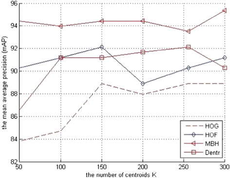
mAP versus the number of centroids K for VLAD
Table 7, we compare two different normalization methods for VLAD on KTH with constrained videos. It shows that the NormalizeCompoents plus SSR have a better result than the NormalizeMass plus SSR, and NormalizeComponets outperforms Normalizemass by one percent of mAP. Hence, in the subsection evaluation, we will use NormalizeComponents plus SSR to normalize the vector for VLAD and SSR for FV.
Table 7 Comparison of different normalized method on KTH with mAP for VLAD (where K = 150) In this section, we will evaluate the combination of descriptors with different aggregating methods. In Table 8 we list different combinations of descriptors with BOW which is obtained from Ref [52]. Table 9 analyze the different combination strategies of FV and VLAD respectively. From those tables, we can see that: in most datasets the more descriptors for combination, the better mAP. While in some special cases, the special combination can achieve the best result such as the KTH in Table 10. For more intuitive comparison, we will evaluate those aggregating methods on KTH.
Table 8 Comparison of different combination of descriptors with mAP for BOW (taken from [52]) Table 9 Comparison of different combination of descriptors with mAP for FV and VLAD (taken from [7]) Table 10 Comparison of different aggregating method for KTH dataset with mAP In Table 10 we evaluate different aggregating methods for KTH dataset and use paper [8] as the baseline. We choose to use one scale for the descriptor of Wang’s paper [53] which they use eight. For FV and VLAD we set K = 256 while K = 4000 of BOW. Linear SVM is used for FV and VLAD while SVM with χ 2 kernel is used for BOW. In Table 10 ‘all combine’ means combining HOG, HOF, MBH and Dentr. From Table 10, it is shown that VLAD and BOW obtain the best result which is 96.3 %. We can conclude from the column of FV and BOW that the result degrades when combining all descriptors. Therefore, we still need to optimize the combination of descriptors and design a suitable fusion method for action recognition in the future. Form the row comparison of the table, it is shown that there has not been a method can be certainly determined which aggregating method should be applied for KTH dataset with constrained videos. We will analyze it for large-scale dataset with realistic videos in the future.

5 Future trends and conclusions
Although significant efforts have been devoted to recognize action with realistic setting during the past few years, the current recognition accuracy for large datasets and unconstrained videos is still far from satisfaction. In this section, we discuss several promising techniques that may improve action recognition performance significantly. How to improve the mAP for the large datasets in the realistic video sequences which is necessary in the real life applications? In the next part we will give several directions which may be used to improve the mAP.
Explore better feature detector and descriptor
There have been many descriptors for action recognition such as 3D-gradient [21], 3D-SIFT [46], etc., and some new descriptors have been proposed in recent years [4, 13, 42, 47, 53, 57]. Some descriptors are along the trajectories, the others are along the interest points (IPs). There are many methods to select or extract IPs. Bilinski et al. [4] proposed a novel figure-centric representation which captured both local density of features and statistics of space-time ordered features. It is novel to consider the space-time order of features. Therefore, it is important to exploit IPs which is representative and discriminative to capture relationships between local features and consider the space-time order of features in the future. Shabani et al. [47] introduced the concept of learning multiple dictionaries of action primitives at different resolutions which they called multiple scale-specific representations. They aimed at exploiting the complementary characteristics of the motions across different scales. Hence, capture complementary information is a trend for all kinds of methods. It is obvious the result from Tables 8, 9, and 10 can improve accuracy when combining with some complementary descriptors.
Design fusion
There have been numerous work for feature fusion [6, 26, 28, 31, 48, 58, 62]. For early and late fusion, they only consider the scenes in the well-constrained condition. From the prior work, it shows that early fusion can more efficiently capture the relationship among features yet it is prone to over-fit the training data. Late fusion deals with the over-fitting problem better but does not allow classifiers to train on all the data at the same time. Hence, double fusion which simply combines early fusion and late fusion together to incorporate their advantages in [59]. The future work will focus on designing a scheme to automatically select and optimize early fusion subset to combine with late fusion and aim at exploring the suitable place to fuse for early fusion. Therefore, it can save storage space and be more efficient.
For early fusion, it has two places to fuse, which is in the local descriptor (place1) or in the mid-level vector (place2). The early fusion often is considered in place2 for different kinds of local descriptor [31, 51, 53]. While the spatio-temporal pyramid often fuses in the place1 such as [51, 53], and sometimes in the place2 [1, 61]. Table 9 shows that place2 (k-level) fusion is better than place1 (d-level) fusion in most cases. In the future we will explore which place to fuse for large-scale action recognition.
Design better aggregating method
As we know that the FV and VLAD begin to use recognizing action with unconstrained videos in 2013. How to design more compact and discriminative FV and VLAD is important for action recognition. Arandijelovic et al. [1] were through three stages to improve the performance of VLAD which were intra-normalization, multi-VLAD and vocabulary adaptation for image retrieval. Delhumeau et al. [9] were through two aspects to re-visite VLAD which are residual normalization and local coordinate system (LCS) for image classification. There are a few researches for action recognition in this field. Ballas et al. [3] proposed a novel pooling strategy for action recognition, which obtained a significant improvement of 62 % for UCF 50. It is obvious that to design a better pooling or coding method can significantly improve both accuracy and efficiency. Therefore, it is important to design a suitable coding or pooling strategy for action recognition with realistic videos.
In the future our goal is to achieve sparse, fast, efficient and robust algorithm. We can design algorithm from the three points discussed in the above section. Furthermore, they are also the main pursuits in computer vision.
References
Arandjelovic R, Zisserman A (2013) All about VLAD. IEEE Conf Comput Vis Pattern Recogn
Atmosukarto I, Ghanem B, Ahuja N (2012) Trajectory-based fisher kernel representation for action recognition in videos. Int Conf Pattern Recogn 3333–3336
Ballas N et al (2013) Space-time robust video representation for action recognition. ICCV
Bilinski P, Bremond F (2012) Contextual statistics of space-time ordered features for human action recognition. In Advanced Video and Signal-Based Surveillance (AVSS), 2012 I.E. Ninth International Conference on. 228–233
Boureau YL et al (2010) Learning mid-level features for recognition. IEEE Conf Comput Vis Pattern Recogn 2559–2566
Bregonzio M et al (2010) Discriminative topics modelling for action feature selection and recognition. BMVC
Cai Z et al (2014) Multi-view super vector for action recognition. CVPR
Cho J et al (2013) Robust action recognition using local motion and group sparsity. Pattern Recogn
Delhumeau J et al (2013) Revisiting the VLAD image representation. In Proceedings of the 21st ACM international conference on multimedia. ACM 653–656
Erol A et al (2007) Vision-based hand pose estimation: a review. Comput Vis Image Underst 108(1):52–73
Fathi A, Mori G (2008) Action recognition by learning mid-level motion features. IEEE Conf Comput Vis Pattern Recogn 1–8
Fei-Fei L, Perona P (2005) A bayesian hierarchical model for learning natural scene categories. IEEE ComputSoc Conf ComputVis Pattern Recogn
Gilbert A, Illingworth J, Bowden R (2009) Fast realistic multi-action recognition using mined dense spatio-temporal features. IEEE Int Conf Comput Vis 925–931
Han D, Bo L, Sminchisescu C (2009) Selection and context for action recognition. IEEE IntConf Comput Vis 1933–1940
Hu W et al (2004) A survey on visual surveillance of object motion and behaviors. IEEE Trans Syst Man Cybern C Appl Rev 34(3):334–352
Jain M, Jégou H, Bouthemy P (2013) Better exploiting motion for better action recognition. Int Conf Comput Vis Pattern Recogn
Jégou H et al (2012) Aggregating local image descriptors into compact codes. IEEE Trans Pattern Anal Mach Intell 34(9):1704–1716
Jégou H et al (2010) Aggregating local descriptors into a compact image representation. IEEE Conf Comput Vis Pattern Recogn 3304–3311
Kim SJ et al (2014) View invariant action recognition using generalized 4D features. Pattern Recogn Lett
Klaser A, Marszalek M (2008) A spatio-temporal descriptor based on 3D-gradients. BMVC
Koniusz P, Yan F, Mikolajczyk K (2013) Comparison of mid-level feature coding approaches and pooling strategies in visual concept detection. Comput Vis Image Underst 117(5):479–492
Kuehne H et al (2011) HMDB: a large video database for human motion recognition. IEEE Int Conf Comput Vis 2556–2563
Lan Z, Bao L, Yu S I, et al (2013) Multimedia classification and event detection using double fusion [J]. Multimedia Tool Appl 1–15
Laptev I (2005) On space-time interest points. Int J Comput Vis 64(2–3):107–123
Laptev I et al (2008) Learning realistic human actions from movies. IEEE Conf Comput Vis Pattern Recogn 1–8
Le QV et al (2011) Learning hierarchical invariant spatio-temporal features for action recognition with independent subspace analysis. IEEE Conf Comput Vis Pattern Recogn
Liu J, Ali S, Shah M (2008) Recognizing human actions using multiple features. IEEE Conf Comput Vis Pattern Recogn 1–8
Liu J, Luo J, Shah M (2009) Recognizing realistic actions from videos “in the wild”. IEEE Conf Comput Vis Pattern Recogn
Liu C et al (2012) Action recognition with discriminative mid-level features. IEEE Int Conf Pattern Recogn 3366–3369
Marszalek M, Laptev I, Schmid C (2009) Actions in context. IEEE Conf Comput Vis Pattern Recogn
Murthy OR, Goecke R (2013) Combined ordered and improved trajectories for large scale human action recognition
Murthy OR, Goecke R (2013) Ordered trajectories for large scale human action recognition. IEEE Int Conf Comput Vis Works
Murthy OR, Radwan I, Goecke R (2014) Dense body part trajectories for human action recognition
Niebles JC, Chen CW, Fei-Fei L (2010) Modeling temporal structure of decomposable motion segments for activity classification [M]//computer vision–ECCV 2010. Springer, Berlin, pp 392–405
Nowak E, Jurie F, Triggs B (2006) Sampling strategies for bag-of-features image classification. Comput Vis–ECCV 2006. Springer. 490–503
Pavlovic VI, Sharma R, Huang TS (1997) Visual interpretation of hand gestures for human-computer interaction: a review. IEEE Trans Pattern Anal Mach Intell 19(7):677–695
Perronnin F, Dance C (2007) Fisher kernels on visual vocabularies for image categorization. IEEE Conf Comput Vis Pattern Recogn 1–8
Perronnin F, Sánchez J, Mensink T (2010) Improving the fisher kernel for large-scale image classification. Comput Vis–ECCV 2010. Springer. 143–156
Ramanathan M, Yau WY, Teoh EK (2014) Human action recognition with video data: research and evaluation challenges. IEEE Trans Hum Mach Syst
Reddy KK, Shah M (2013) Recognizing 50 human action categories of web videos [J]. Mach Vis Appl 24(5):971–981
Roca X (2011) A selective spatio-temporal interest point detector for human action recognition in complex scenes. Int Conf Comput Vis 1776–1783
Rodriguez M, Ahmed J, Shah M (2008) Action MACH: a patio-temporal maximum average correlation height filter for action recognition. IEEE Conf Comput Vis Pattern Recogn
Sadanand S, Corso JJ Action bank: a high-level representation of activity in video. IEEE Conf Comput Vis Pattern Recogn 1234–1241
Schuldt C, Laptev I, Caputo B (2014) Recognizing human actions: a local SVM approach. Proc Int Conf Pattern Recogn 32–36
Scovanner P, Ali S, Shah M (2007) A 3-dimensional sift descriptor and its application to action recognition. In Proceedings of the 15th international conference on Multimedia. ACM 357–360
Shabani AH, Zelek JS, Clausi DA (2013) Multiple scale-specific representations for improved human action recognition. Pattern Recogn Lett 34(15):1771–1779
Snoek CG, Worring M, Smeulders AW (2005) Early versus late fusion in semantic video analysis. In Proceedings of the 13th annual ACM international conference on Multimedia. ACM 399–402
Soomro K, Zamir AR, Shah M (2012) UCF101: a dataset of 101 human actions classes from videos in the wild. arXiv preprint arXiv:1212.0402
Ullah MM, Parizi SN, Laptev I (2010) Improving bag-of-features action recognition with non-local cues. BMVC 95.1–95.11
Wang H, Schmid C (2013) Action recognition with improved trajectories. Int Conf Comput Vis
Wang H et al (2013) Dense trajectories and motion boundary descriptors for action recognition. Int J Comput Vis 1–20
Wang H et al (2011) Action recognition by dense trajectories. IEEE Conf Comput Vis Pattern Recogn
Wang H et al (2009) Evaluation of local spatio-temporal features for action recognition. Br Mach Vis Conf
Weinland D, Ronfard R, Boyer E (2011) A survey of vision-based methods for action representation, segmentation and recognition. Comput Vis Image Underst 115(2):224–241
Willems G, Tuytelaars T, Van Gool L (2008) An efficient dense and scale-invariant spatio-temporal interest point detector [M]//computer vision–ECCV 2008. Springer, Berlin, pp 650–663
Wu S, Oreifej O, Shah M (2011) Action recognition in videos acquired by a moving camera using motion decomposition of lagrangian particle trajectories. IEEE Int Conf Comput Vis
Wu D, Shao L (2013) Silhouette analysis-based action recognition via exploiting human poses. IEEE Trans Circuits Syst Video Technol 23(2):236–243
Wu Q et al (2013) Realistic human action recognition with multimodal feature selection and fusion. IEEE Trans Syst Man Cybern Syst 43(4):875–885
Wu X et al (2011) Action recognition using context and appearance distribution features. IEEE Conf Comput Vis Pattern Recogn 489–496
Xu H, Tian Q, Wang Z et al (2014) Human action recognition using late fusion and dimensionality reduction[C]//Digital Signal Processing (DSP). IEEE Int Conf 63–67
Yan S et al (2012) Beyond spatial pyramids: a new feature extraction framework with dense spatial sampling for image classification. Comp Vis–ECCV 2012. Springer 473–487
Yanai K (2014) A dense SURF and triangulation based spatio-temporal feature for action recognition. MultiMedia Model. Springer 375–387
Zhang J et al (2007) Local features and kernels for classification of texture and object categories: a comprehensive study. Int J Comput Vis 73(2):213–238
Zhang T et al (2011) Boosted exemplar learning for action recognition and annotation. IEEE Trans Circuits Syst Video Technol 21(7):853–866
Zhang T et al (2009) Boosted exemplar learning for human action recognition. IEEE Int Conf Comput Vis Works 538–545
Zhou, X et al (2010) Image classification using super-vector coding of local image descriptors. Comput Vis–ECCV 2010. Springer 141–154
Zhou X et al (2008) Sift-bag kernel for video event analysis. Proceedings of the 16th ACM international conference on Multimedia. ACM 229–238
Acknowledgments
This work was partly supported by the National Science Foundation of China (Grant No.61001104), Key Foundation of Jiangsu (Grant No.BK2011018), the Fundamental Research Funds for the Central Universities and Graduate Research and Innovation Projects of Universities in Jiangsu Province (KYLX_0129)
Author information
Authors and Affiliations
Corresponding author
Rights and permissions
About this article

Cite this article
Xu, H., Tian, Q., Wang, Z. et al. A survey on aggregating methods for action recognition with dense trajectories. Multimed Tools Appl 75, 5701–5717 (2016). https://doi.org/10.1007/s11042-015-2536-2
Received:
Revised:
Accepted:
Published:
Issue Date:
DOI: https://doi.org/10.1007/s11042-015-2536-2