
Abstract
Łukasiewicz presented two different analyses of modal notions by means of many-valued logics: (1) the linearly ordered systems Ł3,...,  ,..., \(\hbox {L}_{\omega }\); (2) the 4-valued logic Ł he defined in the last years of his career. Unfortunately, all these systems contain “Łukasiewicz type (modal) paradoxes”. On the other hand, Brady’s 4-valued logic BN4 is the basic 4-valued bilattice logic. The aim of this paper is to show that BN4 can be strengthened with modal operators following Łukasiewicz’s strategy for defining truth-functional modal logics. The systems we define lack “Łukasiewicz type paradoxes”. Following Brady, we endow them with Belnap–Dunn type bivalent semantics.
1 Introduction
The aim of this paper is to investigate two modal strengthenings of Brady’s paraconsistent 4-valued logic BN4 (cf. Brady 1982). In order to define these modal strengthenings of BN4, we will follow Łukasiewicz’s approach to modal many-valued logics (cf. Łukasiewicz 1951, 1953, 1970). As Minari remarks (cf. Minari 0000), the original motivation and the philosophical significance of Łukasiewicz’s many-valued systems lie in “two strictly intertwined issues”: (1) the rejection of deterministic philosophy; (2) “the aim to provide an adequate logical foundation to modal propositions, and more generally, to the very notions of possibility and necessity” (cf. Minari 0000, p. 1). Thus, for example, Łukasiewicz points out the following about the 3-valued logic Ł3, the first one of the many-valued logics he defined: “The indeterministic philosophy [...] is the metaphysical substratum of the new logic” (Łukasiewicz 1920/1970, p. 88). “The third logical value may be interpreted as “possibility” ” (Łukasiewicz 1920/1970, p. 87).
Łukasiewicz presented two different analyses of modal notions by means of many-valued logics: (a) the linearly ordered systems Ł3,..., Łn,..., Ł\(\omega \) he defined since 1920 (cf. Łukasiewicz 1970; b) the 4-valued modal logic Ł he defined in the last years of his career (cf. Łukasiewicz 1951, 1953). In the family Ł3,..., Łn,..., Ł\(\omega \) the modal operators L (necessity) and M (possibility) can be defined as follows: \(LA=_{\mathrm {df} }\lnot (A\rightarrow \lnot A)\), \(MA=_{\mathrm {df}}\lnot A\rightarrow A\) (these definitions were suggested by Tarski when he was Łukasiewicz’s student; the symbols L and M are Łukasiewicz’s—cf. Font and Hajek (2002), notes 2 and 3; cf. Definition 2.1 on the languages used in this paper). On the other hand, L and M are defined in Ł independently of the rest of the connectives of the system (cf. Łukasiewicz 1951, 1953; Font and Hajek 2002).
Unfortunately, both the systems of the sequence Ł3,...,Łn,...,Ł\(\omega \) and the logic Ł validate such theses as the following (cf. Proposition 3.26 below): (f7) \(L(A\vee B)\rightarrow (LA\vee LB)\) and (f8) \( (MA\wedge MB)\rightarrow M(A\wedge B)\), which are in principle difficult to accept from an intuitive point of view. Moreover, in addition to f7 and f8, the following are provable in Ł: (f5) \((A\rightarrow B)\rightarrow (MA\rightarrow MB)\); (f6) \((A\rightarrow B)\rightarrow (LA\rightarrow LB)\); (f9) \(LA\rightarrow (B\rightarrow LB)\); (f10) \(LA\rightarrow (MB\rightarrow B)\). Theses f9 and f10 are especially counterintuitive, fact that leads the authors of Font and Hajek (2002) to conclude that Ł is a “dead end” as a modal logic of necessity and possibility [the reader can find an analysis of Ł explaining why these counterintuitive consequences arise in the system in Méndez et al. (2015)]. Thus, it must be concluded that neither the family Ł3,...,Łn,...,Ł\(\omega \) nor Ł can be taken as a many-valued analysis of the notions of necessity and possibility when understood in their customary sense. However, the aim of this paper is to show that both strategies followed by Łukasiewicz [(a) and (b) referred to above] work when modally strengthening Brady’s BN4. We mean “work” in the following sense: (1) Łukasiewicz’s type paradoxes such as f5-f10 remarked above are falsified in both strengthenings; (2) both modal strengthenings of BN4 are strong, genuine 4-valued modal logics (cf. Propositions 3.25, 3.26). In order to explain the strengthenings we propose appropriately, we begin by discussing some of the main features of Brady’s BN4.
The logic BN4 was defined by Brady (1982). The matrix MBN4 (cf. Definition 2.7) upon which BN4 is built is, according to Brady (1982, p. 10), a modification of Smiley’s matrix MSm4 (cf. Definition 6.3 in the Appendix), characteristic of Anderson and Belnap’s First Degree Entailment Logic, FDE (cf. Anderson and Belnap 1975, pp. 161–162). According to Dunn (2000, p. 8), the matrix MSm4 is in its turn a simplification of Anderson and Belnap’s 8-element matrix \(\mathrm{M}_{0}\) (cf. Belnap 1960), which has played an important role on the development of relevant logics (cf. Routley et al. 1982, pp. 176, ff.; \(\mathrm{M}_{0}\) is defined in the Appendix—Definition 6.4).
The logic BN4 can be considered as an implicative expansion of Belnap and Dunn’s well known logic B4, which is equivalent to Anderson and Belnap’s logic FDE mentioned above (cf. Belnap 1977a, b; Dunn 1976, 2000 and the references in this last item). That is, BN4 is a strengthening of B4 by introducing \( \rightarrow \) as a new connective (cf. Definition 2.5 on the matrix MB4 upon which the logic B4 is defined). In fact, it is easy to show (cf. “The basic logic \(\mathrm{GBL}_{\supset }\) is BN4” section of the Appendix) that the “strong implication” (\(\rightarrow \)) of the bilattice logic \(\mathrm{GBL}_{\supset }\) (cf. Arieli and Avron 1996, 1998) is actually the conditional of BN4. Now, given that “strong implication” (\(\rightarrow \)) and “weak implication” (\(\supset \)) are interderdefinable in the context of the \(\{\wedge ,\vee ,\lnot \}\) fragment of \(\mathrm{GBL}_{\supset }\) (cf. Arieli and Avron 1996, §3.4), the basic logic \(\mathrm{GBL}_{\supset }\), i.e., the \(\{\rightarrow ,\wedge ,\vee ,\lnot \}\) fragment of \(\mathrm{GBL}_{\supset }\), is actually the logic BN4 defined by Brady. Therefore BN4 is undoubtedly a central non-classical logic.
According to Meyer et al., BN4 “is the correct logic for the 4-valued situation, where the extra values are to be interpreted in the both and neither senses” (Meyer et al. 1984, p. 253). On the other hand, Slaney considers this logic as the truth-functional implication most naturally associated with FDE, i.e., with B4 (cf. Slaney 2005, p. 289).
The label BN4 is explained by Brady as follows (Brady 1982, p. 32, Note 1): “This name is chosen because the system contains the basic system B of Routley et al. 1982, Chapter 4, and has a characteristic 4-valued matrix set, one of the values being ‘n’, representing neither truth nor falsity”. However, it is tempting to read BN4 as B(oth) and N (either) 4-valued logic. That is, as the logic interpreted by the truth values T(ruth) and F(alsity), N (neither T nor F) and B (both T and F), which is precisely as Belnap intuitively interpreted the elements of the 4-element matrix MB4 (cf. Belnap 1960, 1977a).
Two modal strengthenings of BN4 are investigated in the present paper.
-
1.
The logic EBN4, a definitional extension of BN4 defined by introducing L and M in BN4 according to the tarskian definitions \(\lnot (A\rightarrow \lnot A)\) and \(\lnot A\rightarrow A\), respectively.
-
2.
The logic \({\mathcal {M}}\mathrm{BN}4\), a modal expansion of BN4, defined by introducing L and M according to the following truth tables:
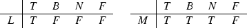

According to these tables, LA is true iff A is true; otherwise LA is false; and MA is false if A is false; otherwise MA is true. We remark that these tables are not definable from the rest of the connectives of BN4 (cf. Proposition 2.9). These tables are investigated in the algebraic study (Font and Rius 2000) briefly commented below, and are one of the sets suggested in Béziau (2011).
There are other modal expansions of B4 (and of its expansions) in the literature. Let us briefly comment on some of them and explain in which sense our proposal is an original one.
Priest (2008) is a modal expansion of the logic FDE by using Kripke models. Odintsov and Wansing (2010) investigate modal implicative expansions of BN4. The basic logics contain classical positive logic with strong negation. Jung and Rivieccio (2013) study a modal expansion of Arieli and Avron’s bilattice logic (in its full language), which has been mentioned above (they expand the full logic \(\mathrm{GBL}_{\supset }\) in the language \(\{\wedge ,\vee ,\otimes ,\oplus ,\supset ,\lnot ,t,f,\top ,\bot \}\)). Font and Rius (2000) is an algebraic investigation of two expansions of B4 based on two different consequence relations defined on the modal expansion of the matrix MB4 (cf. Definition 2.5 below on this matrix). Finally, Goble (2006) investigates normal modal expansions of BN4 and RM3. (RM3 is the strongest extension of R-Mingle; cf. Anderson and Belnap (1975) and Brady (1982)).
As suggested above, our approach is “Łukasiewiczian ” in character and, as such, is fairly different from those adopted in the investigations just briefly commented. Thus, unlike Goble (2006), Jung and Rivieccio (2013), Odintsov and Wansing (2010) and Priest (2008), we shall dispense with “possible worlds” for interpreting the modal operators; and unlike Font and Rius (2000), which investigates modal expansions of MB4, ours is a study of a modal implicative expansion of the same matrix.
The structure of the paper is as follows. In Sect. 2, the 4-valued logics BN4 and \({\mathcal {M}}\mathrm{BN}4\) are defined, Belnap–Dunn type semantics are provided for each one of them and the soundness theorems are proved. In Sect. 3, we prove completeness of BN4 and \({\mathcal {M}}\mathrm{BN}4\) both w.r.t. their matrices MBN4 and \(\mathrm{M}{\mathcal {M}}\mathrm{BN}4\), on the one hand, and their respective Belnap–Dunn type semantics, on the other. In addition, some properties of \({\mathcal {M}}\mathrm{BN}4\) are briefly discussed (for example, that \( {\mathcal {M}}\mathrm{BN}4\) is a conservative extension of BN4). In the first part of Sect. 4, the (modal) definitional extension of BN4, EBN4, is investigated. Then, in the second part, it is shown how to introduce the modal operators of EBN4 in other logics similar to BN4 independently of the tarskian definitions. The paper ends in Sect. 5 with some considerations on the results obtained and on further work on the same topic to be developed in other research papers. We have added an “Appendix” on some technical matters mentioned throughout the paper.
2 Brady’s 4-Valued Logic BN4 and Its Modal Expansion \({\mathcal {M}}\mathrm{BN}4\)
This section is subdivided into three subsections. In the first one, we set some preliminary definitions; in the second one, the modal expansion of Brady’s 4-valued logic BN4, \({\mathcal {M}}\mathrm{BN}4\), is defined; finally, in the third subsection, Belnap–Dunn type semantics for the logic \({\mathcal {M}}\mathrm{BN}4\) is provided.
2.1 Preliminary Definitions
Firstly, we define the logical languages and the notion of logic used in this paper.
Definition 2.1
(Languages) The propositional language consists of a denumerable set of propositional variables \(p_{0},p_{1},\ldots ,p_{n},\ldots ,\) and some or all of the following connectives \(\rightarrow \) (conditional), \(\wedge \) (conjunction), \(\vee \) (disjunction), \(\lnot \) (negation), L (necessity), M (possibility). The biconditional (\(\leftrightarrow \)) and the set of wffs are defined in the customary way. A, B (possibly with subscripts \(0,1,\ldots ,n\)), etc. are metalinguistic variables. By \({\mathcal {P}}\) and \({\mathcal {F}}\), we shall refer to the set of all propositional variables and the set of all wff, respectively.
Definition 2.2
(Logics) A logic S is a structure (L, \(\vdash _{\mathrm {S}})\) where L is a propositional language and \(\vdash _{\mathrm {S}}\) is a (proof-theoretical) consequence relation defined on L by a set of axioms and a set of rules of derivation. The notions of ‘proof’ and ‘theorem’ are understood as it is customary in Hilbert-style axiomatic systems (\({\varGamma } \vdash _{\mathrm {S}}A\) means that A is derivable from the set of wffs \({\varGamma } \) in S; and \(\vdash _{\mathrm {S}}A\) means that A is a theorem of S).
Next, the notion of a logical matrix and related notions are defined.
Definition 2.3
(Logical matrix) A (logical) matrix is a structure \(({\mathcal {V}},D,\mathtt {F})\) where (1) \({\mathcal {V}}\) is a (ordered) set of (truth) values; (2) D is a non-empty proper subset of \({\mathcal {V}}\) (the set of designated values); and (3) \(\mathtt {F}\) is the set of n-ary functions on \({\mathcal {V}}\) such that for each n-ary connective c (of the propositional language in question), there is a function \(f_{c}\in \mathtt {F}\) such that \({\mathcal {V}} ^{n}\rightarrow {\mathcal {V}}\).
Definition 2.4
(M-interpretations, M-consequence, M-validity) Let M be a matrix for (a propositional language) L. An M-interpretation I is a function from \({\mathcal {F}}\) to \({\mathcal {V}}\) according to the functions in \(\mathtt {F}\). Then, for any set of wffs \({\varGamma } \) and wff A, \({\varGamma } \vDash _{\mathrm {M}}A\) (A is a consequence of \({\varGamma } \) according to M) iff \( I(A)\in D\) whenever \(I({\varGamma } )\in D\) for all M-interpretations \(I (I({\varGamma })\in D\) iff \(I(B)\in D\) for each \(B\in {\varGamma })\). In particular, \( \vDash _{\mathrm {M}}A\) (A is M-valid; A is valid in the matrix M) iff \( I(A)\in D\) for all M-interpretations I. (By \(\vDash _{\mathrm {M}}\) we shall refer to the relation defined in M).
We can now define Belnap and Dunn’s 4-element matrix MB4 (cf. Belnap 1977a, b; Dunn 2000 and references therein). As pointed out in the Introduction, Brady’s 4-element matrix MBN4 is an implicative expansion of MB4.
Definition 2.5
(Belnap and Dunn’s matrix MB4) The propositional language consists of the connectives \(\wedge \), \(\vee \) and \(\lnot \). Belnap and Dunn’s matrix MB4 is the structure \(({\mathcal {V}},D,\mathtt {F})\) where (1) \({\mathcal {V}}=\{0,1,2,3\}\) and it is partially ordered as shown in the following diagram

(2) \(D=\{3,2\}\); (3) \(\mathtt {F}=\{f_{\wedge },f_{\vee },f_{\lnot }\}\) where \(f_{\wedge }\) and \(f_{\vee }\) are defined as the glb (or lattice meet) and the lub (or lattice join), respectively. Finally, \(f_{\lnot }\) is an involution with \(f_{\lnot }(0)=3,f_{\lnot }(3)=0,f_{\lnot }(1)=1\) and \( f_{\lnot }(2)=2\). For the reader’s convenience, we display the tables for \( \wedge \), \(\vee \) and \(\lnot \):

The notions of an MB4-interptetation, MB4-consequence and MB4-validity are defined according to the general Definition 2.4.
Remark 2.6
(On the intuitive meaning of the truth values in MB4) The truth values 0, 1, 2 and 3 can intuitively be interpreted in MB4 as follows. Let T and F represent truth and falsity. Then, \(0=F\), \( 1= N\)(either), \(2=B\)(oth) and \(3=T\) (cf. Belnap 1977a, b) Or, in terms of subsets of \(\{T,F\}\), we have: \(0=\{F\}\), \(1=\emptyset \), \(2=\{T,F\}\) and \( 3=\{T\}\) (cf. Dunn 2000 and references therein). It is in this sense that we speak of “bivalent semantics” when referring to the Belnap–Dunn semantics: there are only two truth values and the possibility of assigning both or neither to propositions. (We use the symbols 0, 1, 2 and 3 because they are convenient for using the tester in González (2012) in case the reader needs one.)
2.2 The Logic \({\mathcal {M}}\mathrm{BN}4\)
In this subsection the modal expansion of Brady’s 4-valued logic BN4, \( {\mathcal {M}}\mathrm{BN}4\), is defined. The first step is the definition of Brady’s matrix MBN4, an implicative expansion of MB4. Then, the matrix \(\mathrm{M}{\mathcal {M}}\) BN4, a modal expansion of MBN4, is defined.
Definition 2.7
(Brady’s matrix MBN4) The propositional language consists of the connectives \(\rightarrow \), \( \wedge \), \(\vee \) and \(\lnot \). Brady’s matrix MBN4 is the structure \(( {\mathcal {V}},D,\mathtt {F})\) where (1) \({\mathcal {V}}\) and D are defined as in MB4 (Definition 2.5) and \(\mathtt {F}=\{f_{\rightarrow },f_{\wedge },f_{\vee },f_{\lnot }\}\) where \(f_{\wedge }\), \(f_{\vee }\) and \(f_{\lnot }\) are defined as in MB4 and \(f_{\rightarrow }\) according to the following table:

The related notions of an MBN4-interpretation, etc. are defined according to the general Definition 2.4 [we note that Brady uses the symbols f, n, b, t instead of 0, 1, 2, 3, respectively (cf. Brady 1982, p. 10)].
Definition 2.8
(he matrix \(\mathrm{M}{\mathcal {M}}\mathrm{BN}4\)) The propositional language consists of the connectives \(\rightarrow \), \( \wedge \), \(\vee \), \(\lnot \) and L. By \({\mathcal {M}}\mathrm{BN}4\) we refer to the modal expansion of BN4 defined below in Definition 2.11. The 4-element (modal) matrix \(\mathrm{M}{\mathcal {M}}\mathrm{BN}4\) is the structure \(({\mathcal {V}},D,\mathtt { F})\) where (1) \({\mathcal {V}}\), D and \(\mathtt {F}\) are defined exactly as in the matrix MBN4 except for the addition of the unary function \(f_{L}\), which is defined according to the following table:

As in the preceding cases, the notions of an \(\mathrm{M}{\mathcal {M}}\) BN4-interpretation, etc. are defined according to the general Definition 2.4.
It is important to remark that the necessity function \(f_{L}\) is not definable by using the rest of the functions in the matrix \(\mathrm{M}{\mathcal {M}}\mathrm{BN}4\).
Proposition 2.9
(Non-definabililty of \(f_{L}\)) The function \(f_{L}\) is not definable from the functions \(f_{\rightarrow },f_{\wedge },f_{\vee }\) and \(f_{\lnot }\) in matrix \(\mathrm{M}{\mathcal {M}}\mathrm{BN}4\).
Proof
It suffices to note that \(f_{\rightarrow }(2,2)=f_{\wedge }(2,2)=f_{\vee }(2,2)=f_{\lnot }(2)=2\) and that formulas of the form LA are never assigned the value 2. \(\square \)
In what follows, the logics BN4 and \({\mathcal {M}}\mathrm{BN}4\) are defined.
Definition 2.10
(The logic BN4) The logic BN4 can be axiomatized as follows:
Axioms

Rules of derivation

Brady’s original axiomatization of BN4 (cf. Brady 1982, p. 22) can be found in “Brady’s original axiomatization of BN4” section of the Appendix, where it is proved that the axiomatization of Definition 2.10 is equivalent to it.
Definition 2.11
(The modal logic \({\mathcal {M}}\mathrm{BN}4\)) The modal logic \({\mathcal {M}}\mathrm{BN}4\) is axiomatized when adding the following axioms and definition to BN4:
The notions of ‘derivation’ and ‘theorem’ are understood in a standard sense both in BN4 and \({\mathcal {M}}\mathrm{BN}4\) (cf. Definition 2.2). The following theorems and rule of \({\mathcal {M}}\mathrm{BN}4\) are needed in the completeness proof. We note that T1–T4 are provable in Anderson and Belnap’s FDE (actually, in its positive fragment, \(\mathrm{FDE}_{+}\)) (cf. Anderson and Belnap 1975, §15.2), while T5–T11 are theorems of Contractionless Relevant Logic, RW, which is axiomatized by A1–A10, MP and Adj (cf. for example, Slaney 1987).
Proposition 2.12
(Some theorems of \({\mathcal {M}}\mathrm{BN}4\)) The following theses and rule are provable in \({\mathcal {M}}\mathrm{BN}4\) (a proof is sketched to the right of each one of them):

In Proposition 3.25, we have recorded a selection of significant modal theorems of \({\mathcal {M}}\mathrm{BN}4\). Now, let us note the following definition.
Definition 2.13
(Logics determined by matrices) Let L be a propositional language, M a matrix for L and \(\vdash _{\mathrm {S}}\) a (proof theoretical) consequence relation defined on L. Then, the logic S (cf. Definition 2.2) is determined by M iff for every set of wffs \({\varGamma } \) and wff A, \({\varGamma } \vdash _{\mathrm {S}}A\) iff \({\varGamma } \vDash _{\mathrm {M}}A\). In particular, the logic S (considered as the set of its theorems) is determined by M iff for every wff A, \(\vdash _{\mathrm {S}}A\) iff \(\vDash _{ \text {M}}A\) (cf. Definition 2.4).
In Brady (1982), Brady shows that the logic BN4 (as axiomatized by him—cf. Brady (1982, p. 22) and “Brady’s original axiomatization of BN4” section of the Appendix) is determined by the matrix MBN4. By leaning on Brady’s strategy and proof, we will show, on our part, that the logic \({\mathcal {M}}\mathrm{BN}4\) is determined by the matrix \(\mathrm{M}{\mathcal {M}}\mathrm{BN}4\), that is, that \(\mathrm{M}{\mathcal {M}}\mathrm{BN}4\) is a characteristic matrix for \({\mathcal {M}}\mathrm{BN}4\). A corollary of this fact is that BN4, as axiomatized in Definition 2.10, is determined by MBN4 (cf. Corollary 3.22).
2.3 Belnap–Dunn Type Semantics for \({\mathcal {M}}\mathrm{BN}4\)
In this subsection a Belnap–Dunn type semantics for \({\mathcal {M}}\mathrm{BN}4\) is provided and the soundness theorem is proved. This semantics is “bivalent” in the sense of Remark 2.6. Firstly, \({\mathcal {M}}\mathrm{BN}4\)-models and the notions of \({\mathcal {M}}\)BN4-consequence and \({\mathcal {M}}\mathrm{BN}4\)-validity are defined (cf. Brady 1982, p. 23).
Definition 2.14
(\({\mathcal {M}}\mathrm{BN}4\)-models) An \({\mathcal {M}}\mathrm{BN}4\)-model is a structure (K4, I) where (i) \( K4=\{\{T\},\{F\},\{T,F\},\emptyset \}\); (ii) I is an \({\mathcal {M}}\)BN4-interpretation from \({\mathcal {F}}\) to K4, this notion being defined according to the following conditions for all \(p\in {\mathcal {P}}\) and \(A,B\in {\mathcal {F}}\): (1) \(I(p)\in K4\); (2a) \(T\in I(\lnot A)\) iff \(F\in I(A)\); (2b) \( F\in I(\lnot A)\) iff \(T\in I(A)\); (3a) \(T\in I(A\wedge B)\) iff \(T\in I(A)\) and \(T\in I(B)\); (3b) \(F\in I(A\wedge B)\) iff \(F\in I(A)\) or \(F\in I(B)\); (4a) \(T\in I(A\vee B)\) iff \(T\in I(A)\) or \(T\in I(B)\); (4b) \(F\in I(A\vee B)\) iff \(F\in I(A)\) and \(F\in I(B)\); (5a) \(T\in I(A\rightarrow B)\) iff \((T\notin I(A)\) or \(T\in I(B))\) and (\(F\in I(A)\) or \(F\notin I(B))\); (5b) \(F\in I(A\rightarrow B)\) iff \(T\in I(A)\) and \(F\in I(B)\); (6a) \(T\in I(LA)\) iff \( T\in I(A)\) and \(F\notin I(A)\); (6b) \(F\in I(LA)\) iff \(T\notin I(LA)\).
Definition 2.15
(\({\mathcal {M}}\mathrm{BN}4\)-consequence; \({\mathcal {M}}\mathrm{BN}4\)-validity) For any set of wffs \({\varGamma } \) and wff A, \({\varGamma } \vDash _{\mathrm {M}}A\) (A is a consequence of \({\varGamma } \) in the \({\mathcal {M}}\mathrm{BN}4\)-model M) iff \(T\in I(A) \) if \(T\in I({\varGamma } )\) (\(T\in I({\varGamma } )\) iff \(\forall A\in {\varGamma } (T\in I(A))\); \(F\in I({\varGamma } )\) iff \(\exists A\in {\varGamma } (F\in I(A))\)). In particular, \(\vDash _{\mathrm {M}}A\) (A is true in M) iff \(T\in I(A)\). Then, \( {\varGamma } \vDash _{{\mathcal {M}}\text {BN4}}A\) (A is a consequence of \({\varGamma } \) in \({\mathcal {M}}\mathrm{BN}4\)-semantics) iff \({\varGamma } \vDash _{\mathrm {M}}A\) for each \( {\mathcal {M}}\mathrm{BN}4\)-model M. In particular, \(\vDash _{{\mathcal {M}}\text {BN4}}A\) ( A is valid in \({\mathcal {M}}\mathrm{BN}4\)-semantics) iff \(\vDash _{\mathrm {M}}A\) for each \({\mathcal {M}}\mathrm{BN}4\)-model M (by \(\vDash _{{\mathcal {M}}\text {BN4}}\), we shall refer to the relation just defined).
We note the following remark.
Remark 2.16
(On the clauses for the possibility operator) Notice that, given the definition of the possibility operator M (cf. Definition 2.11), the clauses for M are as follows: (7a) \(T\in I(MA)\) iff \( T\in I(A)\) or \(F\notin I(A)\); (7b) \(F\in I(MA)\) iff \(T\notin I(MA)\).
Now, it is easy to show that \(\vDash _{\mathrm {M}{\mathcal {M}}\text {BN4}}\) (the consequence relation defined in the matrix \(\mathrm{M}{\mathcal {M}}\mathrm{BN}4\); cf. Definition 2.8) and \(\vDash _{{\mathcal {M}}\text {BN4}}\) (the consequence relation just defined in \({\mathcal {M}}\mathrm{BN}4\)-semantics) are coextensive (cf. Brady 1982, p. 24).
Proposition 2.17
(Coextensiveness of \(\vDash _{\mathrm {M}{\mathcal {M}}\text {BN4}}\) and \(\vDash _{{\mathcal {M}}\text {BN4}}\)) For any set of wffs \({\varGamma } \) and wff A, \({\varGamma } \vDash _{\mathrm {M}\mathcal { M}\text {BN4}}A\) iff \({\varGamma } \vDash _{{\mathcal {M}}\text {BN4}}A\). In particular, \(\vDash _{\mathrm {M}{\mathcal {M}}\text {BN4}}A\) iff \(\vDash _{{\mathcal {M}}\text {BN4}}A\).
Proof
Cf. Brady (1982), Theorem 8. \(\square \)
We end this subsection by proving soundness and remarking that the necessitation rule is not only not derivable in \({\mathcal {M}}\mathrm{BN}4\) but also inadmissible in this logic.
Theorem 2.18
(Soundness of \({\mathcal {M}}\mathrm{BN}4\) w.r.t. \(\vDash _{\mathrm {M} {\mathcal {M}}\text {BN4}}\)) For any set of wffs \({\varGamma }\) and wff A, if \({\varGamma } \vdash _{{\mathcal {M}} \text {BN4}}A\), then \({\varGamma } \vDash _{\mathrm {M}{\mathcal {M}}\text {BN4}}A\).
Proof
Induction on the length of the derivation supporting the claim \({\varGamma }\vdash _{{\mathcal {M}}\text {BN4}}A\). The proof is left to the reader. [In case a tester is needed, the reader can use that in González (2012).] \(\square \)
An immediate corollary of Theorem 2.18 is the following:
Corollary 2.19
(Soundness of \({\mathcal {M}}\mathrm{BN}4\) w.r.t. \(\vDash _{{\mathcal {M}} \text {BN4}}\)) For any set of wffs \({\varGamma } \) and wff A, if \({\varGamma } \vdash _{{\mathcal {M}} \text {BN4}}A\), then \({\varGamma } \vDash _{{\mathcal {M}}\text {BN4}}A\).
Proof
Immediate by Proposition 2.17 and Theorem 2.18. \(\square \)
Proposition 2.20
(Inadmissibility of Nec in \({\mathcal {M}}\mathrm{BN}4\)) The rule Necessitation (Nec) \(A \Rightarrow LA\) is not admissible in \( {\mathcal {M}}\mathrm{BN}4\).
Proof
Let \(p_{i}\) be a propositional variable. The wff \(L(p_{i}\rightarrow p_{i})\) is falsified by any \(\mathrm{M}{\mathcal {M}}\mathrm{BN}4\)-interpretation assigning 2 to \(p_{i}\) (cf. Anderson and Belnap 1975, pp. 53–54 on the notions derivable rule and admissible rule). \(\square \)
3 Completeness of \({\mathcal {M}}\mathrm{BN}4\)
In this section, we prove that \({\mathcal {M}}\mathrm{BN}4\) is complete w.r.t. \(\vDash _{ {\mathcal {M}}\text {BN4}}\), the relation defined in \({\mathcal {M}}\mathrm{BN}4\)-semantics (cf. Definition 2.15). Then, completeness w.r.t. \(\vDash _{\mathrm {M}\mathcal {M }\text {BN4}}\), the relation defined in the matrix \(\mathrm{M}{\mathcal {M}}\mathrm{BN}4\) (cf. Definition 2.8) follows immediately by Proposition 2.17. The first subsection investigates properties of \({\mathcal {M}}\mathrm{BN}4\)-theories; the second one is dedicated to the extension and primeness lemmas, and finally, in the third one, canonical models are defined and the completeness theorem is proved.
3.1 \({\mathcal {M}}\mathrm{BN}4\)-Theories
We begin by defining the notion of a \({\mathcal {M}}\mathrm{BN}4\)-theory and the classes of \({\mathcal {M}}\mathrm{BN}4\)-theories considered in this paper.
Definition 3.1
(\({\mathcal {M}}\mathrm{BN}4\)-theories) An \({\mathcal {M}}\mathrm{BN}4\)-theory (theory, for short) is a set of formulas closed under Adjunction (Adj), Modus Ponens (MP), provable \({\mathcal {M}}\)BN4-implication (\({\mathcal {M}}\mathrm{BN}4\)-imp) and Disjunctive Modus Ponens (dMP). That is, \({\mathcal {T}}\) is a theory iff for \(A,B,C\in {\mathcal {F}}\), we have (1) whenever \(A,B\in {\mathcal {T}}\), \(A\wedge B\in {\mathcal {T}}\) (Adj); (2) whenever \(A\rightarrow B\in {\mathcal {T}}\) and \(A\in {\mathcal {T}}\), \(B\in {\mathcal {T}}\) (MP); (3) whenever \(A\rightarrow B\) is a theorem of \({\mathcal {M}} \mathrm{BN}4\) and \(A\in {\mathcal {T}}\), then \(B\in {\mathcal {T}}\) (\({\mathcal {M}}\mathrm{BN}4\)-imp); and (4) whenever \(C\vee (A\rightarrow B)\in {\mathcal {T}}\) and \(C\vee A\in {\mathcal {T}}\), then \(C\vee B\in {\mathcal {T}}\) (dMP).
Definition 3.2
(Classes of theories) Let \({\mathcal {T}}\) be a theory. We set (1) \({\mathcal {T}}\) is prime iff, for \( A,B\in {\mathcal {F}}\), whenever \(A\vee B\in {\mathcal {T}}\), then \(A\in \mathcal {T }\) or \(B\in {\mathcal {T}}\); (2) \({\mathcal {T}}\) is regular iff \({\mathcal {T}}\) contains all theorems of \({\mathcal {M}}\mathrm{BN}4\); (3) \({\mathcal {T}}\) is trivial iff it contains all wffs; finally, (4) \({\mathcal {T}}\) is a-consistent (consistent in an absolute sense) iff \({\mathcal {T}}\) is not trivial.
Next, we record a couple of properties of theories.
Proposition 3.3
(Closure under Modus Tollens) If \({\mathcal {T}}\) is a theory, then it is closed under Modus Tollens (MT). That is, for \(A,B\in {\mathcal {F}}\), if \(A\rightarrow B\in {\mathcal {T}}\) and \( \lnot B\in {\mathcal {T}}\), then \(\lnot A\in {\mathcal {T}}\).
Proof
Let \({\mathcal {T}}\) be a theory and suppose for \(A,B\in {\mathcal {F}}\), \( A\rightarrow B\in {\mathcal {T}}\) and \(\lnot B\in {\mathcal {T}}\). By T7, \(\lnot B\rightarrow \lnot A\in {\mathcal {T}}\), whence \(\lnot A\in {\mathcal {T}}\) by MP. \(\square \)
Lemma 3.4
(Theories and double negation) Let \({\mathcal {T}}\) be a theory. For \(A\in {\mathcal {F}}\), \(A\in {\mathcal {T}}\) iff \(\lnot \lnot A\in {\mathcal {T}}\).
Proof
Immediate by A9 and T6. \(\square \)
In what follows, we turn to prove some properties of prime theories and of a-consistent and/or regular and prime theories.
Lemma 3.5
(Conjunction and disjunction in prime theories) Let \({\mathcal {T}}\) be a prime theory and \(A,B\in {\mathcal {F}}\). Then, (1a) \( A\wedge B\in {\mathcal {T}}\) iff \(A\in {\mathcal {T}}\) and \(B\in {\mathcal {T}}\); (1b) \(\lnot (A\wedge B)\in {\mathcal {T}}\) iff \(\lnot A\in {\mathcal {T}}\) or \( \lnot B\in {\mathcal {T}}\); (2a) \(A\vee B\in {\mathcal {T}}\) iff \(A\in {\mathcal {T}}\) or \(B\in {\mathcal {T}}\); (2b) \(\lnot (A\vee B)\in {\mathcal {T}}\) iff \(\lnot A\in {\mathcal {T}}\) and \(\lnot B\in {\mathcal {T}}\).
Proof
Case 1a: by A4 and fact that \({\mathcal {T}}\) is closed under Adj. Case 1b: by T11 and the fact that \({\mathcal {T}}\) is prime. Case 2a: by A6 and the fact that \({\mathcal {T}}\) is prime. Case 2b: by T10 and the fact that \({\mathcal {T}}\) is closed under Adj. \(\square \)
Lemma 3.6
(The conditional in regular prime theories) Let \({\mathcal {T}}\) be a regular and prime theory and \(A,B\in {\mathcal {F}}\). Then, (1) \(A\rightarrow B\in {\mathcal {T}}\) iff \((A\notin {\mathcal {T}}\) or \(B\in \mathcal {T)}\) and \((\lnot A\in {\mathcal {T}}\) or \(\lnot B\notin \mathcal {T)}\); (2) \(\lnot (A\rightarrow B)\in {\mathcal {T}}\) iff \(A\in {\mathcal {T}}\) and \(\lnot B\in {\mathcal {T}}\).
Proof
(1a) \(A\rightarrow B\in {\mathcal {T}}\Rightarrow \mathcal {(}A\notin {\mathcal {T}} \) or \(B\in {\mathcal {T}})\) and \((\lnot A\in {\mathcal {T}}\) or \(\lnot B\notin {\mathcal {T}})\). Suppose \(A\rightarrow B\in {\mathcal {T}}\) and, for reductio, (i) \(A\in {\mathcal {T}}\) and \(B\notin {\mathcal {T}}\) or (ii) \(\lnot A\notin {\mathcal {T}}\) and \(\lnot B\in {\mathcal {T}}\). But (i) and (ii) are impossible since \({\mathcal {T}}\) is closed under MP and MT (cf. Proposition 3.3). (1b) \( (A\notin {\mathcal {T}}\) or \(B\in \mathcal {T)}\) and \((\lnot A\in {\mathcal {T}}\) or \(\lnot B\notin {\mathcal {T}})\Rightarrow A\rightarrow B\in {\mathcal {T}}\). We have to consider the four alternatives (i)–(iv) below. (i) \(A\notin \mathcal { T}\) and \(\lnot A\in {\mathcal {T}}\). By A12, \(\lnot A\rightarrow [A\vee (A\rightarrow B)]\). So, \(A\vee (A\rightarrow B)\in {\mathcal {T}}\) whence \( A\rightarrow B\in {\mathcal {T}}\) by the primeness of \({\mathcal {T}}\). (ii) \( A\notin {\mathcal {T}}\) and \(\lnot B\notin {\mathcal {T}}\). By A13 and the regularity of \({\mathcal {T}}\), \((A\vee \lnot B)\vee (A\rightarrow B)\in {\mathcal {T}}\). Thus, \(A\rightarrow B\in {\mathcal {T}}\) by the primeness of \( {\mathcal {T}}\). (iii) \(B\in {\mathcal {T}}\) and \(\lnot A\in {\mathcal {T}}\). By A11, \((\lnot A\wedge B)\rightarrow (A\rightarrow B)\). Then, \(A\rightarrow B\in {\mathcal {T}}\) follows immediately. (iv) \(B\in {\mathcal {T}}\) and \(\lnot B\notin {\mathcal {T}}\). Then, \(A\rightarrow B\in {\mathcal {T}}\) follows, similarly as in (1b) (i), by T12 (\(B\rightarrow [\lnot B\vee (A\rightarrow B)]\)). (2a) \(\lnot (A\rightarrow B)\in {\mathcal {T}}\Rightarrow (A\in \mathcal {T }\) and \(\lnot B\in {\mathcal {T}})\). For reductio, suppose \(\lnot (A\rightarrow B)\in {\mathcal {T}}\) but (i) \(A\notin {\mathcal {T}}\) or (ii) \(\lnot B\notin {\mathcal {T}}\). Let us consider case i. By A14, \(A\vee [\lnot (A\rightarrow B)\rightarrow A]\in {\mathcal {T}}\) hence \(\lnot (A\rightarrow B)\rightarrow A\in {\mathcal {T}}\) and, finally, by MP, \(A\in {\mathcal {T}}\), contradicting (i). That (ii) is impossible is similarly shown by using T13 (\( \lnot B\vee [\lnot (A\rightarrow B)\rightarrow \lnot B]\)). (2b) \(( A\in {\mathcal {T}}\) and \(\lnot B\in {\mathcal {T}})\Rightarrow \lnot (A\rightarrow B)\in {\mathcal {T}}\) . By T14, \((A\wedge \lnot B)\rightarrow [(A\wedge \lnot B)\rightarrow \lnot (A\rightarrow B)]\). Then, as \( A\wedge \lnot B\in {\mathcal {T}}\), we have \((A\wedge \lnot B)\rightarrow (A\rightarrow B)\in {\mathcal {T}}\) by \({\mathcal {M}}\mathrm{BN}4\)-imp and \(\lnot (A\rightarrow B)\in {\mathcal {T}}\) by MP. \(\square \)
Lemma 3.7
(The necessity operator in a-cons. reg. prime theories) Let \({\mathcal {T}}\) be an a-consistent, regular and prime theory and \(A\in {\mathcal {F}}\). Then, (1) \(LA\in {\mathcal {T}}\) iff \(A\in {\mathcal {T}}\) and \(\lnot A\notin {\mathcal {T}}\); (2) \(\lnot LA\in {\mathcal {T}}\) iff \(LA\notin {\mathcal {T}}\).
Proof
(1a) \(LA\in {\mathcal {T}}\Rightarrow (A\in {\mathcal {T}}\) and \(\lnot A\notin {\mathcal {T}})\). Suppose \(LA\in {\mathcal {T}}\). By A15 (\(LA\rightarrow A\)), \( A\in {\mathcal {T}}\). Suppose now \(\lnot A\in {\mathcal {T}}\) and let B be an arbitrary wff. By T17 (\(\lnot A\rightarrow \lnot LA\)), \(\lnot LA\in \mathcal { T}\) hence \(LA\wedge \lnot LA\in {\mathcal {T}}\) and, finally, \(B\in {\mathcal {T}}\) by A17 (\((LA\wedge \lnot LA)\rightarrow B\)), contradicting the a-consistency of \({\mathcal {T}}\). (1b) \((A\in {\mathcal {T}}\) and \(\lnot A\notin {\mathcal {T}} )\Rightarrow LA\in {\mathcal {T}}\) . By A15 (\(A\rightarrow (\lnot A\vee LA)\)), \( LA\in {\mathcal {T}}\). (2a) \(\lnot LA\in {\mathcal {T}}\Rightarrow LA\notin {\mathcal {T}}\). Suppose \(\lnot LA\in {\mathcal {T}}\) but \(LA\in {\mathcal {T}}\) and let B be an arbitrary wff. Then \(B\in {\mathcal {T}}\) by A17 (\((LA\wedge \lnot LA)\rightarrow B\)), contradicting the a-consistency of \({\mathcal {T}}\). (2b) \(LA\notin {\mathcal {T}}\Rightarrow \lnot LA\in {\mathcal {T}}\) . It follows immediately by \(LA\vee \lnot LA\) (T18) and the primeness of \( {\mathcal {T}}\). \(\square \)
3.2 Extension and Primeness Lemmas
Firstly, we set a preliminary definition (cf. Brady 1982, pp. 24–25).
Definition 3.8
(Disjunctive \({\mathcal {M}}\mathrm{BN}4\)-derivability) For any sets of wffs \({\varGamma } \), \({\varTheta } \), \({\varTheta } \) is disjunctively derivable from \({\varGamma } \) in \({\mathcal {M}}\mathrm{BN}4\) (in symbols, \({\varGamma } \vdash _{ {\mathcal {M}}\text {BN4}}^{d}{\varTheta } \)) iff \(A_{1}\wedge \ldots \wedge A_{n}\vdash _{{\mathcal {M}}\text {BN4}}B_{1}\vee \ldots \vee B_{m}\) for some wffs \( A_{1},\ldots ,A_{n}\in {\varGamma } \) and \(B_{1},\ldots ,B_{m}\in {\varTheta } \).
Next, we prove a lemma which is essential in order to prove the extension to maximal sets lemma. (In the rest of the section the subscript \({\mathcal {M}}\)BN4 is, in general, dropped from \(\vdash _{{\mathcal {M}}\text {BN4}}\) since no confusion can arise as \({\mathcal {M}}\mathrm{BN}4\) is the only logic treated throughout Sect. 3.)
Lemma 3.9
(Main auxiliary lemma) For any \(A,B_{1},\ldots ,B_{n}\in {\mathcal {F}}\), if \(\{B_{1},\ldots ,B_{n}\}\vdash _{{\mathcal {M}}\text {BN4}}A\), then, for any wff C, \(C\vee (B_{1}\wedge \ldots \wedge B_{n})\vdash _{{\mathcal {M}}\text {BN4}}C\vee A\).
Proof
(Cf. Brady 1982, p. 27) Induction on the length of the proof of A from \( \{B_{1},\ldots ,B_{n}\}\) (H.I abbreviates hypothesis of induction). (1) \(A\in \{B_{1},\ldots ,B_{n}\}\). Let A be \(B_{i}(1\le i\le n)\). By elementary properties of \(\wedge \), \(\vdash (B_{1}\wedge \ldots \wedge B_{n})\rightarrow B_{i}\). By T4 (\(A\rightarrow B\Rightarrow (C\vee A)\rightarrow (C\vee B)\)), \( C\vee (B_{1}\wedge \ldots \wedge B_{n})\vdash C\vee A\). (2) A is an axiom. By A4, \(\vdash C\vee A\). So, \(C\vee (B_{1}\wedge \ldots \wedge B_{n})\vdash C\vee A\) . (3) A is by Adj. Then, A is \(D\wedge E\) for some wffs D and E. By H.I, \(C\vee (B_{1}\wedge \ldots \wedge B_{n})\vdash C\vee D\) and \(C\vee (B_{1}\wedge \ldots \wedge B_{n})\vdash C\vee E\) whence \(C\vee (B_{1}\wedge \ldots \wedge B_{n})\vdash (C\vee D)\wedge (C\vee E)\) by Adj. Finally, \(C\vee (B_{1}\wedge \ldots \wedge B_{n})\vdash C\vee (D\wedge E)\) by T3 (\([A\vee (B\wedge C)]\leftrightarrow [(A\vee B)\wedge (C\vee D)]\)). (4) A is by MP. By H.I, \(C\vee (B_{1}\wedge \ldots \wedge B_{n})\vdash C\vee (D\rightarrow A)\) and \(C\vee (B_{1}\wedge \ldots \wedge B_{n})\vdash C\vee D\) for some wff D. So, \(C\vee (B_{1}\wedge \ldots \wedge B_{n})\vdash C\vee A\) by dMP. (5) A is by dMP. Then, A is \(D\vee E\) for some wffs D and E. By H.I, \(C\vee (B_{1}\wedge \ldots \wedge B_{n})\vdash C\vee (D\vee F)\) and \(C\vee (B_{1}\wedge \ldots \wedge B_{n})\vdash C\vee [D\vee (F\rightarrow E)]\) for some wff F, whence \(C\vee (B_{1}\wedge \ldots \wedge B_{n})\vdash (C\vee D)\vee F\) and \(C\vee (B_{1}\wedge \ldots \wedge B_{n})\vdash (C\vee D)\vee (F\rightarrow E)\) by T2 (\([A\vee (B\vee C)\leftrightarrow [(A\vee B)\vee C]\)). So, \(C\vee (B_{1}\wedge \ldots \wedge B_{n})\vdash (C\vee D)\vee E\) by dMP and, finally, \(C\vee (B_{1}\wedge \ldots \wedge B_{n})\vdash C\vee (D\vee E)\) by T2, as it was required in case 5, which ends the proof of Lemma 3.9. \(\square \)
Now, we proceed to show how to extend sets of wffs to maximal sets [cf. Lemma 9 in Brady (1982) and Chapter 4 in Routley et al. (1982)].
Definition 3.10
(Maximal sets) \({\varGamma } \) is a maximal set of wffs iff \({\varGamma } \nvdash ^{d}{\overline{{\varGamma }}} \) (\({\overline{{\varGamma }}}\) is the complement of \({\varGamma } \)).
Lemma 3.11
(Extension to maximal sets) Let \({\varGamma } \), \({\varTheta } \) be sets of wffs such that \({\varGamma } \nvdash ^{d}{\varTheta } \). Then, there are sets of wffs \({\varGamma } ^{\prime }\), \({\varTheta } ^{\prime }\) such that \({\varGamma } \subseteq {\varGamma } ^{\prime }\), \({\varTheta } \subseteq {\varTheta } ^{\prime }\), \({\varTheta } ^{\prime }={\overline{{\varGamma }}}^{\prime } \) and \({\varGamma } ^{\prime }\nvdash ^{d}{\varTheta } ^{\prime }\) (that is, \({\varGamma } ^{\prime }\) is a maximal set such that \({\varGamma } ^{\prime }\nvdash ^{d}{\varTheta } ^{\prime }\)).
Proof
Let \(A_{1},\ldots ,A_{n},\ldots ,\) be an enumeration of the wffs. The sets \({\varGamma } ^{\prime }\) and \({\varTheta } ^{\prime }\) are defined as follows: \({\varGamma } ^{\prime }=\displaystyle \bigcup \limits _{k\in {\mathbb {N}} }{\varGamma } _{k}\), \({\varTheta } ^{\prime }=\displaystyle \bigcup \limits _{k\in {\mathbb {N}} }{\varTheta } _{k}\) where \({\varGamma } _{0}={\varGamma } \), \({\varTheta } _{0}={\varTheta } \) and for each \(k\in {\mathbb {N}} \), \({\varGamma } _{k+1}\) and \({\varTheta } _{k+1}\) are defined as follows: (i) if \( {\varGamma } _{k}\cup \{A_{k+1}\}\vdash ^{d}{\varTheta } _{k}\), then \({\varGamma } _{k+1}={\varGamma } _{k}\) and \({\varTheta } _{k+1}={\varTheta } _{k}\cup \{A_{k+1}\}\); (ii) if \({\varGamma } _{k}\cup \{A_{k+1}\}\nvdash ^{d}{\varTheta } _{k}\), then \({\varGamma } _{k+1}={\varGamma } _{k}\cup \{A_{k+1}\}\) and \({\varTheta } _{k+1}={\varTheta } _{k}\). Notice that \({\varGamma } \subseteq {\varGamma } ^{\prime }\), \({\varTheta } \subseteq {\varTheta } ^{\prime }\) and that \({\varGamma } ^{\prime }\cup {\varTheta } ^{\prime }={\mathcal {F}}\). We prove (I) \({\varGamma } _{k}\nvdash ^{d}{\varTheta } _{k}\) for all \(k\in {\mathbb {N}} \). We proceed by reductio ad absurdum. So, suppose that for some \(i\in {\mathbb {N}} \), (II) \({\varGamma } _{i}\nvdash ^{d}{\varTheta } _{i}\) but \({\varGamma } _{i+1}\vdash ^{d}{\varTheta } _{i+1}\). We then consider the two possibilities (i) and (ii) above according to which \({\varGamma } _{i+1}\) and \({\varTheta } _{i+1}\) are defined: (a) \({\varGamma } _{i}\cup \{A_{i+1}\}\nvdash ^{d}{\varTheta } _{i}\). By (ii), \({\varGamma } _{i+1}={\varGamma } _{i}\cup \{A_{i+1}\}\) and \({\varTheta } _{i+1}={\varTheta } _{i}\). By the reductio hypothesis (II), \({\varGamma } _{i}\cup \{A_{i+1}\}\vdash ^{d}{\varTheta } _{i}\) , a contradiction. (b) \({\varGamma } _{i}\cup \{A_{i+1}\}\vdash ^{d}{\varTheta } _{i}\). By (i), \({\varGamma } _{i+1}={\varGamma } _{i}\) and \({\varTheta } _{i+1}={\varTheta } _{i}\cup \{A_{i+1}\}\). By the reductio hypothesis (II), (1) \({\varGamma } _{i}\vdash ^{d}{\varTheta } _{i}\cup \{A_{i+1}\}\). Now, let the formulas of \({\varGamma } _{i}\) and \({\varTheta } _{i}\) in this derivation be \(B_{1},\ldots ,B_{m}\) and \(C_{1},\ldots ,C_{n}\), respectively, and let us refer by B to \(B_{1}\wedge \ldots \wedge B_{n}\) and by C to \(C_{1}\vee \ldots \vee C_{n}\). Then (1) can be rephrased as follows (2) \(B\vdash C\vee A_{i+1}\). On the other hand, given the hypothesis (b), there is a conjunction \(B^{\prime }\) of elements of \({\varGamma } _{i}\) and some disjunction \(C^{\prime }\) of elements of \({\varTheta } _{i}\) such that (3) \( B^{\prime }\wedge A_{i+1}\vdash C^{\prime }\). Let us now refer by \(B^{\prime \prime }\) to \(B\wedge B^{\prime }\) and by \(C^{\prime \prime }\) to \(C\vee C^{\prime }\); we will show (III) \(B^{\prime \prime }\vdash C^{\prime \prime } \), that is, \({\varGamma } _{i}\vdash ^{d}{\varTheta } _{i}\), contradicting the reductio hypothesis and thus proving (I). By elementary properties of \( \wedge \) and \(\vee \), we have (4) \(B^{\prime \prime }\wedge A_{i+1}\vdash C^{\prime \prime }\) from (3), and (5) \(B^{\prime \prime }\vdash C^{\prime \prime }\vee A_{i+1} \) from (2). By (5), we get (6) \(B^{\prime \prime }\vdash C^{\prime \prime }\vee (B^{\prime \prime }\wedge A_{i+1})\) and by (4) and Lemma 3.9, (7) \(C^{\prime \prime }\vee (B^{\prime \prime }\wedge A_{i+1})\vdash C^{\prime \prime }\vee C^{\prime \prime }\) whence by T1 (\( A\leftrightarrow (A\vee A)\)), we have (8) \(C^{\prime \prime }\vee (B^{\prime \prime }\wedge A_{i+1})\vdash C^{\prime \prime }\). By (6) and (8) we get (III) \(B^{\prime \prime }\vdash C^{\prime \prime }\), that is, \({\varGamma } _{i}\vdash ^{d}{\varTheta } _{i}\), contradicting the reductio hypothesis. Consequently, (I) (\({\varGamma } _{k}\nvdash ^{d}{\varTheta } _{k}\) for all \(k\in {\mathbb {N}} \)) is proved. Thus, we have sets of wffs \({\varGamma } ^{\prime }\), \({\varTheta } ^{\prime }\) such that \({\varGamma } \subseteq {\varGamma } ^{\prime }\), \({\varTheta } \subseteq {\varTheta } ^{\prime }\), \({\varTheta } ^{\prime }={\overline{{\varGamma }}}^{\prime } \) and \({\varGamma } ^{\prime }\nvdash ^{d}{\varTheta } ^{\prime }\) (since \({\varGamma } _{k}\nvdash ^{d}{\varTheta } _{k}\) for all \(k\in {\mathbb {N}} \)) and \({\varTheta } ^{\prime }={\overline{{\varGamma }}}^{\prime }\) (since \({\varGamma } ^{\prime }\cap {\varTheta } ^{\prime }=\emptyset \)—otherwise \({\varGamma } _{i}\vdash ^{d}{\varTheta } _{i}\) for some \(i\in {\mathbb {N}} \)—and \({\varGamma } ^{\prime }\cup {\varTheta } ^{\prime }={\mathcal {F}}\)), as it was required. Finally, notice that \({\varGamma } ^{\prime }\) is maximal (since \({\varGamma } ^{\prime }\nvdash ^{d}{\overline{{\varGamma }}}\)). \(\square \)
Before proving the primeness lemma we pause a second to remark the essential role Lemma 3.9 has played in the proof of the extension lemma just given (notice that the rest of syntactical moves required in the said proof can be carried on by leaning on the simple resources of the positive fragment of Anderson and Belnap’s First Degree Entailment Logic FDE—cf. Anderson and Belnap (1975, §15.2), about this logic).
Lemma 3.12
(Primeness) If \({\varGamma } \) is a maximal set, then it is a prime theory.
Proof
(Cf. Lemma 8 in Brady 1982) (1) \({\varGamma } \) is a theory: It is trivial to prove that \( {\varGamma } \) is a theory. For example, let us prove that \({\varGamma } \) is closed under dMP. For reductio, suppose that there are wffs A, B, C such that \( C\vee A\in {\varGamma } \), \(C\vee (A\rightarrow B)\in {\varGamma } \) but \(C\vee B\notin {\varGamma } \). Then, \((C\vee A)\wedge [C\vee (A\rightarrow B)]\vdash C\vee (A\rightarrow B)\) and \((C\vee A)\wedge [C\vee (A\rightarrow B)]\vdash C\vee A\), whence \((C\vee A)\wedge [C\vee (A\rightarrow B)]\vdash C\vee B\) by dMP, contradicting the maximality of \({\varGamma } \). (2) \({\varGamma } \) is prime: If there are some wffs A, B such that \(A\vee B\in {\varGamma } \) but \( A\notin {\varGamma } \) and \(B\notin {\varGamma } \), then \({\varGamma } \) is not maximal by virtue of A1 (\((A\vee B)\rightarrow (A\vee B)\)). \(\square \)
3.3 Canonical Models: Completeness
We shall define the notion of a canonical model and prove that each wff which is not a theorem of \({\mathcal {M}}\mathrm{BN}4\) is falsified in some canonical model. The concept of a canonical model is based upon the notion of a \( {\mathcal {T}}\)-interpretation.
Definition 3.13
(\({\mathcal {T}}\)-interpretations) Let K4 be the set \(\{\{T\},\{F\},\{T,F\},\emptyset \}\) as in Definition 2.14. And let \({\mathcal {T}}\) be an a-consistent, regular and prime theory. Then, the function I from \({\mathcal {F}}\) to K4 is defined as follows: for each \(p\in {\mathcal {P}}\), we set (a) \(T\in I(p)\) iff \(p\in {\mathcal {T}}\); (b) \( F\in I(p)\) iff \(\lnot p\in {\mathcal {T}}\). Next, I assigns a member of K4 to each \(A\in {\mathcal {F}}\) according to conditions 2, 3, 4, 5 and 6 in Definition 2.14. Then, it is said that I is a \({\mathcal {T}}\)-interpretation. (As in Definition 2.14, \(T\in I({\varGamma } )\) iff \(\forall A\in {\varGamma } (T\in I(A))\); \(F\in I({\varGamma } )\) iff \(\exists A\in {\varGamma } (F\in I(A))\).)
Definition 3.14
(Canonical \({\mathcal {M}}\mathrm{BN}4\)-models) A canonical \({\mathcal {M}}\mathrm{BN}4\)-model is a structure \((K4,I_{{\mathcal {T}}})\) where K4 is defined as in Definition 2.14 (or as in Definition 3.13) and \( I_{{\mathcal {T}}}\) is a \({\mathcal {T}}\)-interpretation built upon an a-consistent, regular and prime theory \({\mathcal {T}}\).
Definition 3.15
(The canonical relation \(\vDash _{{\mathcal {T}}}\)) Let \((K4,I_{{\mathcal {T}}})\) be a canonical model, the canonical relation \( \vDash _{{\mathcal {T}}}\) is defined as follows. For any set of wffs \({\varGamma } \) and wff A, \({\varGamma } \vDash _{{\mathcal {T}}}A\) iff \(T\in I_{{\mathcal {T}}}(A)\) if \(T\in I_{{\mathcal {T}}}({\varGamma } )\). In particular, \(\vDash _{{\mathcal {T}}}A\) ( A is true in the canonical \({\mathcal {M}}\mathrm{BN}4\)-model \((K4,I_{{\mathcal {T}}})\)), iff \(T\in I_{{\mathcal {T}}}(A)\).
By Definitions 2.14 and 3.14, it is clear that any canonical \({\mathcal {M}}\)BN4-model is a \({\mathcal {M}}\mathrm{BN}4\)-model.
Proposition 3.16
(Any canonical \({\mathcal {M}}\mathrm{BN}4\)-model is a \({\mathcal {M}}\)BN4-model) Let M \(=(K4,I_{{\mathcal {T}}})\) be a canonical \({\mathcal {M}}\)BN4-model. Then, M is indeed a \({\mathcal {M}}\mathrm{BN}4\)-model.
Proof
It follows immediately by Definitions 2.14 and 3.14 (by the way, notice that each propositional variable—and so, each wff A—can be assigned \(\{T\},\{F\},\{T,F\}\) or \(\emptyset \), since \({\mathcal {T}}\) is required to be a-consistent but neither complete nor consistent in the classical sense). \(\square \)
The following lemma generalizes conditions a and b in Definition 3.13 to the set \({\mathcal {F}}\) of all wffs.
Lemma 3.17
(\({\mathcal {T}}\)-interpreting the set of wffs \({\mathcal {F}}\)) Let I be a \({\mathcal {T}}\)-interpretation defined on the theory \({\mathcal {T}}\) . For each \(A\in {\mathcal {F}}\), we have: (1) \(T\in I(A)\) iff \(A\in {\mathcal {T}} \); (2) \(F\in I(A)\) iff \(\lnot A\in {\mathcal {T}}\).
Proof
Induction on the length of A (the clauses cited in points (a), (b), (c), (d), (e) and (f) below refer to the clauses in Definitions 3.13–2.14—H.I abbreviates “hypothesis of induction”). (a) A is a propositional variable: by conditions (a) and (b) in Definition 3.13. (b) A is of the form \(\lnot B\): (i) \(T\in I(\lnot B)\) iff (clause 2a) \(F\in I(B)\) iff (H.I) \(\lnot B\in {\mathcal {T}}\). (ii) \(F\in I(\lnot B)\) iff (clause 2b) \(T\in I(B)\) iff (H.I) \( B\in {\mathcal {T}}\) iff (Lemma 3.4) \(\lnot \lnot B\in {\mathcal {T}}\). (c) A is of the form \(B\wedge C\): (i) \(T\in I(B\wedge C)\) iff (clause 3a) \(T\in I(B)\) and \(T\in I(C)\) iff (H.I) \(B\in {\mathcal {T}}\) and \(C\in {\mathcal {T}}\) iff (Lemma 3.5) \(B\wedge C\in {\mathcal {T}}\). (ii) \(F\in I(B\wedge C)\) iff (clause 3b) \(F\in I(B)\) or \(F\in I(C)\) iff (H.I) \(\lnot B\in {\mathcal {T}}\) or \(\lnot C\in {\mathcal {T}}\) iff (Lemma 3.5) \(\lnot (B\wedge C)\in {\mathcal {T}}\). (d) A is of the form \(B\vee C\): the proof is similar to (c) by using clauses 4a, 4b and Lemma 3.5. (e) A is of the form \(B\rightarrow C\): (i) \(T\in I(B\rightarrow C)\) iff (clause 5a) \((T\notin I(A)\) or \(T\in I(B))\) and \((F\in I(A)\) or \(F\notin I(B))\) iff (H.I) \((A\notin {\mathcal {T}}\) or \(B\in {\mathcal {T}})\) and \((\lnot A\in {\mathcal {T}}\) or \(\lnot B\notin {\mathcal {T}})\) iff (Lemma 3.6) \(B\rightarrow C \in {\mathcal {T}}\). (ii) \(F\in I(B\rightarrow C) \) iff (clause 5b) \(T\in I(A)\) and \(F\in I(B)\) iff (H.I) \(A\in {\mathcal {T}}\) and \(\lnot B\in {\mathcal {T}}\) iff (Lemma 3.6) \(\lnot (B\rightarrow C)\in {\mathcal {T}}\). (f) A is of the form LB: (i) \(T\in I(LB)\) iff (clause 6a) \( T\in I(B)\) and \(F\notin I(B)\) iff (H.I) \(B\in {\mathcal {T}}\) and \(\lnot B\notin {\mathcal {T}}\) iff (Lemma 3.7) \(LB\in {\mathcal {T}}\). (ii) \(F\in I(LB)\) iff (clause 6b) \(T\notin I(LB)\) iff (Lemma 3.7) \(\lnot LB\in {\mathcal {T}}\). \(\square \)
In what follows, we prove completeness.
Definition 3.18
(The set \(\mathrm{Cn}{\varGamma } [{\mathcal {M}}\mathrm{BN}4]\) ) The set of consequences in \({\mathcal {M}}\mathrm{BN}4\) of a set of wffs \({\varGamma } \) (in symbols \(\mathrm{Cn}{\varGamma } [{\mathcal {M}}\mathrm{BN}4]\) ) is defined as follows: \(\mathrm{Cn} {\varGamma } [{\mathcal {M}}\mathrm{BN}4]=\{A\mid {\varGamma } \vdash _{{\mathcal {M}}\text {BN4 }}A\}\) (cf. Definitions 2.2 and 2.11).
We note the following remark.
Remark 3.19
( \(\mathrm{Cn}{\varGamma } [{\mathcal {M}}\mathrm{BN}4]\) is a regular theory) It is obvious that for any \({\varGamma } \), \(\mathrm{Cn}{\varGamma } [{\mathcal {M}}\mathrm{BN}4]\) is closed under the rules of \({\mathcal {M}}\mathrm{BN}4\) and contains all theorems of this logic. Consequently, it is closed under \({\mathcal {M}}\mathrm{BN}4\)-imp.
Theorem 3.20
(Completeness of \({\mathcal {M}}\mathrm{BN}4\) w.r.t. \(\vDash _{{\mathcal {M}} \text {BN4}}\)) For any set of wffs \({\varGamma } \) and wff A, if \({\varGamma } \vDash _{{\mathcal {M}}\text {BN4}}A\), then \({\varGamma } \vdash _{{\mathcal {M}}\text {BN4}}A\).
Proof
For some set of wffs \({\varGamma }\) and wff A suppose \({\varGamma } \nvdash _{ {\mathcal {M}}\text {BN4}}A\). We prove \({\varGamma } \nvDash _{{\mathcal {M}}\text {BN4}}A\). If \({\varGamma }\nvdash _{{\mathcal {M}}\text {BN4}}A\), then \(A\notin \) \(\mathrm{Cn}{\varGamma } [{\mathcal {M}}\mathrm{BN}4]\). Thus, \(\mathrm{Cn}{\varGamma } [{\mathcal {M}}\mathrm{BN}4]\nvdash _{{\mathcal {M}}\text {BN4}}^{d}\{A\}\): otherwise \(B_{1}\wedge \ldots \wedge B_{n}\vdash _{{\mathcal {M}}\text {BN4}}A\) for some \(B_{1},\ldots B_{n}\in \) \(\mathrm{Cn} {\varGamma } [{\mathcal {M}}\mathrm{BN}4]\), whence A would be in \(\mathrm{Cn}{\varGamma } [{\mathcal {M}}\mathrm{BN}4]\) after all. Then, by Lemma 3.11, there is a maximal set \( {\varGamma } ^{\prime }\) such that \(\mathrm{Cn}{\varGamma } [{\mathcal {M}}\mathrm{BN}4]\subseteq {\varGamma } ^{\prime }\). So, \({\varGamma } \subseteq {\varGamma }^{\prime }\) (since \({\varGamma } \subseteq \) \(\mathrm{Cn}{\varGamma } [{\mathcal {M}}\mathrm{BN}4]\)) and \(A\notin {\varGamma }^{\prime }\). By Lemma 3.12 \({\varGamma } ^{\prime }\) is a prime theory; moreover \( {\varGamma } ^{\prime }\) is regular since \(\mathrm{Cn}{\varGamma } [{\mathcal {M}}\mathrm{BN}4]\) is regular, and it is a-consistent since \(A\notin {\varGamma } ^{\prime }\). Thus, \( {\varGamma } ^{\prime }\) generates a \({\mathcal {T}}\)-interpretation \(I_{{\varGamma } ^{\prime }}\) such that, by Lemma 3.17, \(T\in I_{{\varGamma } ^{\prime }}({\varGamma } )\) (since \(T\in I_{{\varGamma } ^{\prime }}({\varGamma } ^{\prime })\)) but \(T\notin I_{{\varGamma } ^{\prime }}(A)\). So, \({\varGamma } \nvDash _{{\varGamma } ^{\prime }}A\) by Definition 3.15, whence \({\varGamma } \nvDash _{{\mathcal {M}}\text {BN4}}A\) by Definition 2.15 and Proposition 3.16. \(\square \)
We have the following corollaries.
Corollary 3.21
(Strong sound. and comp. w.r.t. \(\vDash _{{\mathcal {M}}\text { BN4}}\) and \(\vDash _{\mathrm {M}{\mathcal {M}}\text {BN4}}\)) For any set of wffs \({\varGamma } \) and wff A, we have (1) \({\varGamma } \vdash _{ {\mathcal {M}}\text {BN4}}A\) iff \({\varGamma } \vDash _{{\mathcal {M}}\text {BN4}}A\); (2) \( {\varGamma } \vdash _{{\mathcal {M}}\text {BN4}}A\) iff \({\varGamma } \vDash _{\mathrm {M} {\mathcal {M}}\text {BN4}}A\).
Proof
(1) By Corollary 2.19 and Theorem 3.20. (2) By Theorems 2.18 and 3.20 with Proposition 2.17. \(\square \)
Notice that throughout the completeness proof developed in this section, the modal axioms A15-A17 (cf. Definition 2.11) have been used only in Proposition 3.7 (‘The necessity operator in a-consistent, prime regular theories’), proposition which in its turn is used in the proof of the clauses concerning the necessity operator in Proposition 3.17 (‘\({\mathcal {T}}\)-interpreting the set of wffs \({\mathcal {F}}\)’). That BN4 (as axiomatized in Definition 2.10) is sound and complete w.r.t. \(\vDash _{\mathrm {MBN4}}\) and that \({\mathcal {M}}\mathrm{BN}4\) is a conservative expansion of BN4 follow from this fact.
Now let a BN4-model be a structure (K4, I) where K4 and I are defined similarly as in a \({\mathcal {M}}\mathrm{BN}4\)-model (Definition 2.14) except that clauses 6a and 6b for the modal operator are dropped. Then, define the relation \(\vDash _{\mathrm {BN4}}\) similarly as the relation \(\vDash _{\mathcal { M}\text {BN4}}\) was defined (Definition 2.15). Then, we record the following corollaries.
Corollary 3.22
(Soundness and completeness of BN4) For any set of wffs \({\varGamma } \) and wff A, \({\varGamma } \vdash _{\mathrm {BN4}}A\) iff \({\varGamma } \vDash _{\mathrm {MBN4}}A\) iff \({\varGamma } \vDash _{\mathrm {BN4}}A\).
Proof
Given the fact remarked above, soundness follows from Theorem 2.18 and Corollary 2.19, and completeness by Corollary 3.21. \(\square \)
Corollary 3.23
(\({\mathcal {M}}\mathrm{BN}4\) is a conservative extension of BN4) The logic \({\mathcal {M}}\mathrm{BN}4\) is a conservative extension of BN4. That is, if \(\vDash _{ {\mathcal {M}}\text {BN4}}A\) and L does not appear in A, then \(\vDash _{ \text {BN4}}A\).
Proof
As pointed out above, it follows from the soundness and completeness proofs of \({\mathcal {M}}\mathrm{BN}4\) and BN4. \(\square \)
The section is ended with some remarks.
We have seen that the rule Nec (Necessitation) is not admissible in \( {\mathcal {M}}\mathrm{BN}4\) (Proposition 2.20). The ‘replacement theorem’, however, holds in this logic.
Proposition 3.24
(The replacement theorem) For any wffs A, B if \(\vdash _{{\mathcal {M}}\text {BN4}}A\leftrightarrow B\), then \(\vdash _{{\mathcal {M}}\text {BN4}}C[A]\leftrightarrow C[A/B]\) (C[A] is a wff in which A appears; C[A / B] is the result of substituting A by B in one or more places in which A occurs).
Proof
By induction on the length of C[A] since if \(\vdash _{{\mathcal {M}}\text {BN4} }A\leftrightarrow B\), then, for any \(C\in {\mathcal {F}}\), (a) \(\vdash _{ {\mathcal {M}}\text {BN4}}(C\wedge A)\leftrightarrow (C\wedge B)\), (b) \(\vdash _{ {\mathcal {M}}\text {BN4}}(C\vee A)\leftrightarrow (C\vee B)\), (c) \(\vdash _{ {\mathcal {M}}\text {BN4}}\lnot A\leftrightarrow \lnot B\) and (d) \(\vdash _{ {\mathcal {M}}\text {BN4}}LA\leftrightarrow LB\) are admissible rules in \( {\mathcal {M}}\mathrm{BN}4\) (the thesis \((A\rightarrow B)\rightarrow (LA\rightarrow LB)\) , for example, fails only when A is assigned 3 and B is assigned 1). \(\square \)
Next, we note some provable and unprovable wffs in \({\mathcal {M}}\mathrm{BN}4\) [in case a tester is needed, the reader can use that in González (2012)].
Proposition 3.25
(Some modal theses provable in \({\mathcal {M}}\mathrm{BN}4\)) The following are provable in \({\mathcal {M}}\mathrm{BN}4\): (t1) \(LA\leftrightarrow \lnot M\lnot A\); (t2) \(MA\leftrightarrow \lnot L\lnot A\); (t3) \( LA\rightarrow A\); (t4) \(A\rightarrow MA\); (t5) \(LA\rightarrow LLA\); (t6) \( MMA\rightarrow MA\); (t7) \(MA\rightarrow LMA\); (t8) \(MLA\rightarrow LA\); (t9) \(L(A\wedge B)\leftrightarrow (LA\wedge LB)\); (t10) \(M(A\vee B)\leftrightarrow (MA\vee MB)\); (t11) \(L(A\rightarrow B)\rightarrow (LA\rightarrow LB)\); (t12) \(M(A\rightarrow B)\rightarrow (LA\rightarrow MB)\) ; (t13) \((MA\rightarrow LB)\rightarrow L(A\rightarrow B)\); (t14) \((LA\vee LB)\rightarrow L(A\vee B)\); (t15) \(M(A\wedge B)\rightarrow (MA\wedge MB)\); (t16) \(L(A\vee B)\rightarrow (LA\vee MB)\); (t17) \((MA\wedge LB)\rightarrow M(A\wedge B)\); (t18) \(A\vee \lnot LA\); (t19) \(\lnot A\vee MA\); (t20) \( (LA\wedge \lnot A)\rightarrow B\); (t21) \(B\rightarrow (A\vee \lnot LA)\); (t22) \((\lnot LA\wedge A)\rightarrow \lnot A\); (t23) \((MA\wedge \lnot A)\rightarrow A\); (t24) \(\lnot A\rightarrow (A\vee \lnot MA)\).
Proof
Theses t1–t24 are verified by any \(\mathrm{M}{\mathcal {M}}\mathrm{BN}4\)-interpretation. Then, they are provable by the completeness theorem (Corollary 3.21). \(\square \)
Notice that theses t1–t21, as well as A15 and A17, are provable in Lewis’ system S5 (when \(\rightarrow \) is interpreted as the material conditional); t22–t24 and A16 are, however, not provable in this logic. Actually, it is easy to see that addition of any of them to S5 would cause the collapse of S5 into classical propositional logic.
We record some wffs not provable in \({\mathcal {M}}\mathrm{BN}4\).
Proposition 3.26
(Some modal wffs not provable in \({\mathcal {M}}\mathrm{BN}4\)) The following are not provable in \({\mathcal {M}}\mathrm{BN}4\): (f1) \(A\rightarrow LA\); (f2) \(MA\rightarrow A\); (f3) \(LMA\rightarrow A\); (f4) \(A\rightarrow MLA\), (f5) \((A\rightarrow B)\rightarrow (MA\rightarrow MB)\); (f6) \((A\rightarrow B)\rightarrow (LA\rightarrow LB)\); (f7) \(L(A\vee B)\rightarrow (LA\vee LB)\); (f8) \((MA\wedge MB)\rightarrow M(A\wedge B)\); (f9) \(LA\rightarrow (B\rightarrow LB)\); (f10) \(LA\rightarrow (MB\rightarrow B)\); (f11) \( (LA\rightarrow MB)\rightarrow M(A\rightarrow B)\); (f12) \((MA\rightarrow MB)\rightarrow M(A\rightarrow B)\).
Proof
Formulas f1–f12 are falsified in the matrix \(\mathrm{M}{\mathcal {M}}\mathrm{BN}4\). Then, they are not provable by the soundness theorem (Corollary 3.21). \(\square \)
The schemes f5–f10 are labelled ‘Łukasiewicz-type paradoxes’ (cf. Méndez et al. (2015) and references therein). So, \({\mathcal {M}}\mathrm{BN}4\) is free from this type of paradoxes. On the other hand, notice that (when \(\rightarrow \) is read as the material conditional) f11 and f12 are provable in Feys-von Wright modal system T (so they are provable in Lewis’ systems S4 and S5). In sum, Propositions 3.25 and 3.26 support the conclusion that \({\mathcal {M}}\mathrm{BN}4\) can be understood as a strong and genuine (4-valued) modal logic.
Finally, we note that the logic \({\mathcal {M}}\mathrm{BN}4\) is paraconsistent.
Proposition 3.27
(\({\mathcal {M}}\mathrm{BN}4\) is paraconsistent) The logic \({\mathcal {M}}\mathrm{BN}4\) is paraconsistent, that is, the rule Ecq (‘E contradiction quodlibet’) \(A,\lnot A\Rightarrow B\) is not provable in \( {\mathcal {M}}\mathrm{BN}4\).
Proof
Let \(p_{i}\), \(p_{m}\) be propositional variables and I be an \(\mathrm{M}{\mathcal {M}}\) BN4-interpretation such that \(I(p_{i})=2\) and \(I(p_{m})=1\). Then, \( \{p_{i},\lnot p_{i}\}\nvDash _{\mathrm {M}{\mathcal {M}}\text {BN4}}p_{m}\). So, Ecq does not hold in \({\mathcal {M}}\mathrm{BN}4\). \(\square \)
However, notice that if a theory contains a formula of the form LA and its negation, this theory collapses into triviality, as A17 indicates.
4 The Logic EBN4
4.1 A Definitional Extension of BN4: The Logic EBN4
The logic EBN4 is a definitional extension of BN4. Following Tarski’s suggestion for introducing the modal operators L and M in Łukasiewicz’s many-valued logics (cf. Font and Hajek 2002, Notes 2 and 3), we set the following definition in BN4.
Definition 4.1
(Tarskian definitions of L and M) For any wff A: (DfL) \(LA=_{\mathrm {df}}\lnot (A\rightarrow \lnot A)\); (Df\( M)MA=_{\mathrm {df}}\lnot A\rightarrow A\).
Then, notice that we have \(MA\leftrightarrow \lnot L\lnot A\), \( LA\leftrightarrow \lnot M\lnot A\) and the rule Nec (Necessitation) \( A\Rightarrow LA\), since \(A\Rightarrow \lnot (A\rightarrow \lnot A)\) is an admissible rule in BN4. Moreover, the following propositions are provable.
Proposition 4.2
(Modal theses provable in EBN4) The following theses in Proposition 3.25 are also provable in EBN4: t1–t15, t18, t19, t22–t24. In addition, f11 and f12 in Proposition 3.26 are also provable although they are not provable in \({\mathcal {M}}\mathrm{BN}4\).
Proof
Similar to that of Proposition 3.25 by using Definition 4.1. \(\square \)
Proposition 4.3
(Some modal wffs not provable in EBN4) The following wffs in Proposition 3.26 are not provable in EBN4: f1–f10. In addition, theses t16, t17, t20 and t21 in Proposition 3.25, which are provable in \({\mathcal {M}}\mathrm{BN}4\), are not provable in EBN4.
Proof
Similar to that of Proposition 3.26 by using Definition 4.1. \(\square \)
Recall that t1–t21 as well as f11, f12 and Nec hold in S5, while t22–t24 (along with f1–f10) are not provable in this logic (if \(\rightarrow \) is understood to represent the material conditional). Thus, EBN4 lacks Łukasiewicz type paradoxes unlike it is the case with Łukasiewicz’s many-valued logics when the modal operators are introduced according to the tarskian suggestions recalled in Definition 4.1.
We note that the tables for L and M in EBN4 are as follows:

And the clauses in Belnap–Dunn type semantics are: (\(6\mathrm{a}^{\prime }\)) \(T\in I(LA)\) iff \(T\in I(A)\); (\(6\mathrm{b}^{\prime }\)) \(F\in I(LA)\) iff \(F\in I(A)\) or \( T\notin I(A)\). Now, the clauses for L in \({\mathcal {M}}\mathrm{BN}4\) are (cf. Definition 2.14): (6a) \(T\in I(LA)\) iff \(T\in I(A)\) and \(F\notin I(A)\); (6b) \(F\in I(LA)\) iff \(T\notin I(LA)\). Therefore, the essential difference between the meaning of L in \({\mathcal {M}}\mathrm{BN}4\) and EBN4 is that if \(I(A)= B \)(oth), LA is assigned B(oth) in the latter logic while it is F (alse) in the former. This fact is reflected in the following proposition.
Proposition 4.4
(Relationship between \({\mathcal {M}}\mathrm{BN}4\) and EBN4) We have \(\vdash _{{\mathcal {M}}\text {BN4}}LA\rightarrow \lnot (A\rightarrow \lnot A)\) but \(\nvdash _{{\mathcal {M}}\text {BN4}}\lnot (A\rightarrow \lnot A)\rightarrow LA\).
Proof
By the soundness and completeness theorems (Corollary 3.21). \(\square \)
4.2 The Logics \(\mathrm{BN}4^{\prime }\) and \({\mathcal {M}}\mathrm{BN}4^{\prime }\)
We think that it is interesting to remark that clauses \(6\mathrm{a}^{\prime }\) and 6b\(^{\prime }\) recorded above can be shown to work canonically if the following axioms and rules are available: \(LA\rightarrow A\), \(A\vee \lnot LA\), \( (LA\wedge \lnot LA)\rightarrow \lnot A\), Nec and Disjunctive Necessitation dNec. So, L and M can be introduced in any logic similar to BN4 and interpretable with Belnap–Dunn type semantics, provided the quoted axioms and rules are present. Let us end this section by examining, as a way of an example, the logic \(\mathrm{BN}4^{\prime }\), a variant of BN4, and its modal expansion \({\mathcal {M}}\mathrm{BN}4^{\prime }\).
Definition 4.5
(The logic \(\mathrm{BN}4^{\prime }\)) The logic \(\mathrm{BN}4^{\prime }\) is axiomatized when adding to BN4 the axiom A18 \( (\lnot A\vee B)\vee \lnot (A\rightarrow B)\) (not provable in BN4) and substituting the axioms (not provable in \(\mathrm{BN}4^{\prime }\)) A11 and A14 by A19 \((\lnot A\wedge B)\rightarrow [(\lnot A\wedge B)\rightarrow (A\rightarrow B)]\) and A20 \(\lnot A\rightarrow [\lnot B\vee [\lnot (A\rightarrow B)\rightarrow \lnot B]]\), respectively.
Next, we define the modal expansion \({\mathcal {M}}\mathrm{BN}4^{\prime }\) of BN4\( ^{\prime }\) according to the suggestions briefly discussed above and remark some theorems of \({\mathcal {M}}\mathrm{BN}4^{\prime }\).
Definition 4.6
(The modal logic \({\mathcal {M}}\mathrm{BN}4^{\prime }\)) The logic \({\mathcal {M}}\mathrm{BN}4^{\prime }\) is axiomatized when adding the following axioms, rules and definition to \(\mathrm{BN}4^{\prime }\): A15 \( LA\rightarrow A\), A21 \(A\vee \lnot LA\), A22 \((LA\wedge \lnot LA)\rightarrow \lnot A\), Necessitation (Nec) \(A\Rightarrow LA\), Disjunctive Necessitation (dNec) \(B\vee A\Rightarrow B\vee LA\), Definition (Possibility) \(MA=_{\mathrm {df }}\lnot L\lnot A\).
Proposition 4.7
(Some theorems of \({\mathcal {M}}\mathrm{BN}4^{\prime }\)) The following are provable in \({\mathcal {M}}\mathrm{BN}4^{\prime }\): T1–T12, T14–T18 of \({\mathcal {M}}\mathrm{BN}4\) (cf. Proposition 2.12). And, in addition, T19 \( B\rightarrow [A\vee [\lnot (A\rightarrow B)\rightarrow A]]\).
Proof
T1–T12, T14–T18 are proved similarly as in Proposition 2.12. Next, T19 is proved by A9, A20, T6, T7 and T9. \(\square \)
Consider now the following matrices which are variants of MBN4 and \(\mathrm{M}{\mathcal {M}}\mathrm{BN}4\).
Definition 4.8
(The matrix \(\mathrm{MBN}4^{\prime }\)) The matrix \(\mathrm{MBN}4^{\prime }\) is defined exactly as the matrix MBN4 (cf. Definition 2.7) except for the function \(f_{\rightarrow }\) which is now defined according to the following truth table:

Definition 4.9
(The matrix \(\mathrm{M}{\mathcal {M}}\mathrm{BN}4^{\prime }\)) The matrix \(\mathrm{M}{\mathcal {M}}\mathrm{BN}4^{\prime }\) is defined exactly as the matrix M\( {\mathcal {M}}\mathrm{BN}4\) (Definition 2.8) except for the functions \(f_{\rightarrow }\) and \(f_{L}\). The former is defined as in the matrix \(\mathrm{MBN}4^{\prime }\) while the latter is defined according to the following truth-table:

Notice that the tarskian definitions do not work in \(\mathrm{BN}4^{\prime }\) since L and M are equivalently defined by the following truth table:

On the other hand, the question whether the table in Definition 4.9 is definable from the rest of the connectives of \(\mathrm{BN}4^{\prime }\) is not important here because \({\mathcal {M}}\mathrm{BN}4^{\prime }\) is introduced as a mere example.
The proof of the soundness theorems is left to the reader. On our part, we shall sketch a proof that \(\mathrm{BN}4^{\prime }\) (\({\mathcal {M}}\mathrm{BN}4^{\prime }\)) is determined by the matrix \(\mathrm{MBN}4^{\prime }\) (\(\mathrm{M}{\mathcal {M}}\mathrm{BN}4^{\prime }\)) (cf. Definition 2.13). We follow the pattern set in Sect. 3 for proving completeness of BN4 and \({\mathcal {M}}\mathrm{BN}4\). The idea is to provide Belnap–Dunn type models for \({\mathcal {M}}\mathrm{BN}4^{\prime }\) and next to define canonical models upon regular and prime theories (a-consistency is not needed in the case of \({\mathcal {M}}\mathrm{BN}4^{\prime }\)). By using the extension and primeness lemmas, it is then shown that each non theorem of \(\mathrm{BN}4^{\prime }\) (\(\mathcal { M}\mathrm{BN}4^{\prime }\)) fails to belong to some regular and prime theory; that is, it is shown that each non theorem of \(\mathrm{BN}4^{\prime }\) (\({\mathcal {M}}\mathrm{BN}4^{\prime }\)) is not true in some canonical model.
As just pointed out, the first step is to define a Belnap–Dunn type semantics for \({\mathcal {M}}\mathrm{BN}4^{\prime }\). Then, some slight modifications of some of the lemmas in Sect. 3 will suffice.
Definition 4.10
(\({\mathcal {M}}\mathrm{BN}4^{\prime }\)-models) \({\mathcal {M}}\mathrm{BN}4^{\prime }\)-models are defined similarly as \({\mathcal {M}}\)BN4-models (Definition 2.14) except that clauses 5b, 6a and 6b are replaced by the following clauses: (\(5\mathrm{b}^{\prime }\)) \(F\in I(A\rightarrow B)\) iff \( (T\in I(A)\) and \(F\in I(B))\) or \((F\notin I(A)\) and \(T\notin I(B))\); (6a\( ^{\prime }\)) \(T\in I(LA)\) iff \(T\in I(A)\); (\(6\mathrm{b}^{\prime }\)) \(F\in I(LA)\) iff \(F\in I(A)\) or \(T\notin I(A)\).
The notions of \({\mathcal {M}}\mathrm{BN}4^{\prime }\)-consequence and \({\mathcal {M}}\mathrm{BN}4^{\prime }\)-validity are defined similarly as in \({\mathcal {M}}\mathrm{BN}4\)-models (cf. Definition 2.15). In what follows Lemmas 3.6, 3.7, 3.9 and 3.12 are slightly reformulated. Firstly we need to modify the notion of a theory.
Definition 4.11
(\({\mathcal {M}}\mathrm{BN}4^{\prime }\)-theories) An \({\mathcal {M}}\mathrm{BN}4^{\prime }\)-theory (theory, for short) is a set of formulas closed under Adj, MP, \({\mathcal {M}}\mathrm{BN}4^{\prime }\)-imp, as in the case of \({\mathcal {M}}\mathrm{BN}4\)-theories (cf. Definition 3.1) and, in addition, by Necessitation (Nec) and Disjunctive Necessitation (dNec) (a theory \(\mathcal { T}\) is closed under Nec iff for \(A\in {\mathcal {F}}\), if \(A\in {\mathcal {T}}\), then \(LA\in {\mathcal {T}}\); a theory \({\mathcal {T}}\) is closed under dNec iff for \(A,B\in {\mathcal {F}}\), if \(B\vee A\in {\mathcal {T}}\), then \(B\vee LA\in {\mathcal {T}}\)).
Next, we prove Lemma 4.12. This lemma modifies Lemma 3.6.
Lemma 4.12
( \(\rightarrow \) in regular and prime theories) Let \({\mathcal {T}}\) be a regular and prime theory and \(A,B\in {\mathcal {F}}\). Then, (1) \(A\rightarrow B\in {\mathcal {T}}\) iff \((A\notin {\mathcal {T}}\) or \( B\in \mathcal {T)}\) and \((\lnot A\in {\mathcal {T}}\) or \(\lnot B\notin \mathcal { T)}\); (2) \(\lnot (A\rightarrow B)\in {\mathcal {T}}\) iff \((A\in {\mathcal {T}}\) and \(\lnot B\in {\mathcal {T}})\) or \((\lnot A\notin {\mathcal {T}}\) and \(B\notin {\mathcal {T}}\)).
Proof
It is similar to that of Lemma 3.6. So, it will suffice to record the theorems of \(\mathrm{BN}4^{\prime }\) used in each case. Case 1: (a) the fact that theories are closed under MP and MT; (b) A12 (\(\lnot A\rightarrow [A\vee (A\rightarrow B)]\)), A13 (\((A\vee \lnot B)\vee (A\rightarrow B)\)), A19 (\((\lnot A\wedge B)\rightarrow [(\lnot A\wedge B)\rightarrow (A\rightarrow B)]\)) and T12 (\(B\rightarrow [\lnot B\vee (A\rightarrow B)]\)). Case 2: (a) T15 (\([\lnot (A\rightarrow B)\wedge \lnot A]\rightarrow A\) ), T16 (\([\lnot (A\rightarrow B)\wedge B]\rightarrow \lnot B\)); A20 (\(\lnot A\rightarrow [\lnot B\vee [\lnot (A\rightarrow B)\rightarrow \lnot B]]\)) and T19 (\(B\rightarrow [A\vee [\lnot (A\rightarrow B)\rightarrow A]]\)); (b) T14 (\((A\wedge \lnot B)\rightarrow [(A\wedge \lnot B)\rightarrow \lnot (A\rightarrow B)]\)) and A18 (\((\lnot A\vee B)\vee \lnot (A\rightarrow B)\)). \(\square \)
Lemma 4.13 below substitutes former Lemma 3.7. (Notice that \({\mathcal {T}}\) needs not be a-consistent.)
Lemma 4.13
(L in regular and prime theories) Let \({\mathcal {T}}\) be a regular and prime theory and \(A\in {\mathcal {F}}\). Then, (1) \(LA\in {\mathcal {T}}\) iff \(A\in {\mathcal {T}}\); (2) \(\lnot LA\in {\mathcal {T}}\) iff \(\lnot A\in {\mathcal {T}}\) or \(A\notin {\mathcal {T}}\).
Proof
(1) Immediate by A15 (\(LA\rightarrow A\)) and the fact that \({\mathcal {T}}\) is closed under Nec. (2a) \(\lnot LA\in {\mathcal {T}}\Rightarrow (\lnot A\in {\mathcal {T}}\) or \(A\notin \mathcal {T)}\). Suppose \(\lnot LA\in {\mathcal {T}}\) and, for reductio, \(\lnot A\notin {\mathcal {T}}\) and \(A\in {\mathcal {T}}\). As \( {\mathcal {T}}\) is closed under Nec, \(LA\wedge \lnot LA\in {\mathcal {T}}\), whence, by A22 (\((LA\wedge \lnot LA)\rightarrow \lnot A\)), \(\lnot A\in {\mathcal {T}}\), a contradiction. (2b) \((\lnot A\in {\mathcal {T}}\) or \(A\notin \mathcal {T)}\Rightarrow \lnot LA\in {\mathcal {T}}\) . Immediate by T17 (\( \lnot A\rightarrow \lnot LA\)) and A21 (\(A\vee \lnot LA\)) together with the primeness of \({\mathcal {T}}\). \(\square \)
Lemma 4.14 adds to Lemma 3.9 the clauses corresponding to the rules Nec and dNec.
Lemma 4.14
(Main auxiliary lemma) For any \(A,B_{1},\ldots ,B_{n}\in {\mathcal {F}}\), if \(\{B_{1},\ldots ,\) \(B_{n}\}\vdash _{{\mathcal {M}}\text {BN4}^{\prime }}A\), then, for any \(C\in {\mathcal {F}}\), \(C\vee (B_{1}\wedge \ldots \wedge B_{n})\vdash _{{\mathcal {M}}\text { BN4}^{\prime }}C\vee A\).
Proof
If (1) \(A\in \{B_{1},\ldots ,B_{n}\}\), (2) A is an axiom, (3) A is by Adj, (4) A is by MP or (5) A is for dMP, the proof is similar to that of Lemma 3.9. So, let us consider the cases where A is by Nec and by dNec. (6) A is by Nec: then, A is LD for \(D\in {\mathcal {F}}\); by H.I, \(C\vee (B_{1}\wedge \ldots \wedge B_{n})\vdash _{{\mathcal {M}}\text {BN4}^{\prime }}C\vee D \). Then, \(C\vee (B_{1}\wedge \ldots \wedge B_{n})\vdash _{{\mathcal {M}}\text {BN4} ^{\prime }}C\vee LD\) by dNec. (7) A is by dNec: then, A is \(D\vee LE\) for \(D,E\in {\mathcal {F}}\). By H.I, \(C\vee (B\wedge \ldots \wedge B_{n})\vdash _{ {\mathcal {M}}\text {BN4}^{\prime }}C\vee (D\vee E)\). Similarly as in case 5 of Lemma 3.9, we have \(C\vee (B\wedge \ldots \wedge B_{n})\vdash _{{\mathcal {M}}\text { BN4}^{\prime }}(C\vee D)\vee E\). So, \(C\vee (B\wedge \ldots \wedge B_{n})\vdash _{{\mathcal {M}}\text {BN4}^{\prime }}(C\vee D)\vee LE\) by dNec and, finally, \( C\vee (B\wedge \ldots \wedge B_{n})\vdash _{{\mathcal {M}}\text {BN4}^{\prime }}C\vee (D\vee LE)\) by T2, as it was required. \(\square \)
The following lemma, Lemma 4.15, modifies the primeness lemma, Lemma 3.12.
Lemma 4.15
(Primeness) If \({\varGamma } \) is a maximal set, then it is a prime theory.
Proof
Given the proof of Lemma 3.12, it remains to prove that \({\varGamma } \) is closed under Nec and dNec, which is immediate. For example, let us consider dNec. Suppose that there are wffs A, B such that \(B\vee A\in {\varGamma } \) but \(B\vee LA\notin {\varGamma } \). As \(B\vee A\vdash _{{\mathcal {M}}\text {BN4}^{\prime }}B\vee A\), \(B\vee A\vdash _{{\mathcal {M}}\text {BN4}^{\prime }}B\vee LA\), by dNec, contradicting the maximality of \({\varGamma } \). \(\square \)
Finally, a modification of Lemma 3.17 has to be considered.
Lemma 4.16
(\({\mathcal {T}}\)-interpreting the set of wffs \({\mathcal {F}}\)) Let I be a \({\mathcal {T}}\)-interpretation defined on the theory \({\mathcal {T}}\) . For each \(A\in {\mathcal {F}}\), we have: (1) \(T\in I(A)\) iff \(A\in {\mathcal {T}} \); (2) \(F\in I(A)\) iff \(\lnot A\in {\mathcal {T}}\).
Proof
Cases (e) and (f) of Lemma 3.17 have to be modified. But the required modifications are immediate by using Lemmas 4.12 and 4.13 in a similar way to which Lemmas 3.6 and 3.7 were used in the proof of Lemma 3.17. \(\square \)
Once the required modifications are done, completeness follows similarly, as in the cases of BN4 and \({\mathcal {M}}\mathrm{BN}4\) (details are left to the reader). Thus, we end the section by stating the following theorems.
Theorem 4.17
(Soundness and completeness of \(\mathrm{BN}4^{\prime }\)) For any set of wffs \({\varGamma } \) and wff A, \({\varGamma } \vdash _{\mathrm {BN4}^{\prime }}A\) iff \( {\varGamma } \vDash _{\mathrm {BN4}^{\prime }}A\) iff \({\varGamma } \vDash _{\mathrm {MBN4} ^{\prime }}A\).
Theorem 4.18
(Soundness and completeness of \({\mathcal {M}}\mathrm{BN}4^{\prime }\)) For any set of wffs \({\varGamma } \) and wff A, \({\varGamma } \vdash _{{\mathcal {M}}\text { BN4}^{\prime }}A\) iff \({\varGamma } \vDash _{{\mathcal {M}}\text {BN4}^{\prime }}A\) iff \({\varGamma } \vDash _{\mathrm {M}{\mathcal {M}}\text {BN4}^{\prime }}A\).
5 Conclusions
In the present paper it has been shown that Łukasiewicz’s strategies for defining truth-functional modal logics work in the context of an important 4-valued logic, Brady’s paraconsistent logic BN4. As it was noted in the introduction to this paper, that these strategies work means on the one hand that Łukasiewicz type paradoxes are avoided and, on the other hand, that the resulting modal logics are not unworthy of consideration. Nevertheless, the question whether these strategies can be applied to other 4-valued logics suggests itself. In this sense, we note a couple of remarks. As it was pointed out in the Introduction, Brady viewed BN4 as a 4-valued extension of Routley and Meyer’s basic logic B. Actually, BN4 is axiomatized by extending DW, the result of extending B with the contraposition axioms (in B, contraposition holds only as a rule of inference) (cf. Routley et al. 1982, Chapter 4, on these and other weak relevant logics. Cf. the axiomatization of Brady’s BN4 in “Brady?s original axiomatization of BN4” section of the Appendix). Now, suppose that the following entries are fixed in the truth table for the conditional but the blank spaces can be filled with any truth-value:

Then, the following three implicative tables (in addition to that of BN4) are the only ones satisfying the axioms and rules of B:

It would then be interesting to investigate how the modal operators behave in the logics resulting from modifying BN4 with these implicative tables, and even to discuss whether any of them can advantageously substitute the implicative table characteristic of BN4.
Another interesting question is the following. Łukasiewicz’s 4-valued modal logic Ł is based upon a matrix whose implicative table satisfies the axioms of classical implicative logic (cf. “Łukasiewicz matrix MŁ” section of the Appendix). As remarked above, the logic Ł has what has been labelled ‘Łukasiewicz type paradoxes’. However, it is possible to build a truth-functional modal logic upon positive classical logic without suffering these paradoxes. One such possibility is studied in Méndez and Robles (2015) where the truth tables for \(\lnot \) and L in Łukasiewicz’s matrix MŁ (cf. “Łukasiewicz matrix MŁ” section in the Appendix) are substituted by the following:

That is, by the \(\lnot \) and L tables in \(\mathrm{M}{\mathcal {M}}\mathrm{BN}4\) (cf. Definition 2.8). But there are undoubtedly other possibilities for introducing \(\lnot \) and L in classical positive logic without having to accept Łukasiewicz type paradoxes into the bargain.
References
Anderson, A. R., & Belnap, N. D., Jr. (1975). Entailment: The logic of relevance and necessity (Vol. I). Princeton: Princeton University Press.
Arieli, O., & Avron, A. (1996). Reasoning with logical bilattices. Journal of Logic, Language and Information, 5, 25–63.
Arieli, O., & Avron, A. (1998). The value of the four values. Artificial Intelligence, 102, 97–141.
Belnap, N. D. (1960). Entailment and relevance. The Journal of Symbolic Logic, 25, 388–389.
Belnap, N. D. (1977a). How a computer should think. In G. Ryle (Ed.), Contemporary aspects of philosophy (pp. 30–55). Stocksfield: Orielv Press Ltd.
Belnap, N. D. (1977b). A useful four-valued logic. In J. M. Dunn & G. Epstein (Eds.), Modern uses of multiple-valued logic (pp. 8–37). Dordrecht: D. Reidel Publishing Co.
Béziau, J. (2011). A new four-valued approach to modal logic. Logique et Analyse, 54, 18–33.
Brady, R. T. (1982). Completeness proofs for the systems RM3 and BN4. Logique et Analyse, 25, 9–32.
Brady, R. T. (Ed.). (2003). Relevant logics and their rivals (Vol. II). Aldershot: Ashgate.
Dunn, J. M. (1976). Intuitive semantics for first-degree entailments and ‘coupled trees’. Philosophical Studies, 29, 149–168.
Dunn, J. M. (2000). Partiality and its dual. Studia Logica, 65, 5–40.
Font, J. M., & Hajek, P. (2002). On Łukasiewicz four-valued modal logic. Studia Logica, 70(2), 157–182.
Font, J. M., & Rius, M. (2000). An abstract algebraic logic approach to tetravalent modal logics. Journal of Symbolic Logic, 65(2), 481–518.
Goble, L. (2006). Paraconsistent modal logic. Logique et Analyse, 193, 3–29.
González, C. (2012). MaTest. http://ceguel.es/matest. Last access 06 June 2015.
Jung, A., & Rivieccio, U. (2013). Kripke semantics for modal bilattice logic (extended abstracts). In Proceedings of the 28th annual ACM/IEEE symposium on logic in computer science (pp. 438–447). IEEE Computer Society Press.
Łukasiewicz, J. (1920/1970). On three-valued logic. In L. Borkowski (Ed.), Jan ŁSelected works (pp. 87–88). Amsterdam: North-Holland Pub. Co.
Łukasiewicz, J. (1951). Aristotle’s syllogistic from the standpoint of modern formal logic. Oxford: Clarendon Press.
Łukasiewicz, J. (1953). A system of modal logic. The Journal of Computing Systems, 1, 111–149.
Łukasiewicz, J. (1970). Selected works. In L. Borkowski (Ed.). Amsterdam: North-Holland Pub. Co.
Méndez, J. M., & Robles, G. (2015). A strong and rich 4-valued modal logic without Łukasiewicz-type paradoxes. Logica Universalis, 9(4), 501–522.
Méndez, J. M., Robles, G., & Salto, F. (2015). An interpretation of Łukasiewicz’s 4-valued modal logic. Journal of Philosophical Logic,. doi:10.1007/s10992-015-9362-x.
Meyer, R. K., Giambrone, S., & Brady, R. T. (1984). Where gamma fails. Studia Logica, 43, 247–256.
Minari, P. (Manuscript). A note on Łukasiewicz’s three-valued logic. http://www.philos.unifi.it/upload/sub/Materiali/Preprint/wajsberg
Odintsov, S. P., & Wansing, H. (2010). Modal logics with Belnapian truth values. Journal of Applied Non-classical Logics, 20, 279–301.
Priest, G. (2008). Many-valued modal logics: A simple approach. Review of Symbolic Logic, 1, 190–203.
Routley, R., Meyer, R. K., Plumwood, V., & Brady, R. T. (1982). Relevant logics and their rivals (Vol. 1). Atascadero, CA: Ridgeview Publishing Co.
Slaney, J. K. (2005). Relevant logic and paraconsistency. In L. Bertossi, A. Hunter, & T. Schaub (Eds.), Inconsistency Tolerance, Lecture Notes in Computer Science (Vol. 3300, pp. 270–293).
Slaney, J. K. (1987). Reduced models for relevant logics without WI. Notre Dame Journal of Formal Logic, 28, 395–407.
Tkaczyk, M. (2011). On axiomatization of Łukasiewicz’s four-valued modal logic. Logic and Logical Philosophy, 20(3), 215–232.
Acknowledgments
Work supported by research project FFI2014-53919-P financed by the Spanish Ministry of Economy and Competitiveness. We sincerely thank an anonymous referee of the JoLLI for his (her) comments and suggestions on a previous draft of this paper.
Author information
Authors and Affiliations
Corresponding author
Appendix
Appendix
1.1 Brady’s Original Axiomatization of BN4
Brady formulated BN4 with the following axioms, rules and definition.
Axioms:

Rules:

Definition:
Let us label \(\mathrm{BN}4_{0}\) Brady’s original formulation. Then, we have:
Proposition 6.1
(\(\mathrm{BN}4_{0}\) and BN4 are deductively equivalent) The logic \(\mathrm{BN}4_{0}\) and BN4 (as defined in Definition 2.10) are deductively equivalent. That is, for \(A\in {\mathcal {F}}\), \(\vdash _{\mathrm {BN4}}A\) iff \( \vdash _{\mathrm {BN4}_{0}}A.\)
Proof
(a) If \(\vdash _{\mathrm {BN4}}A\), then \(\vdash _{\mathrm {BN4}_{0}}A\). It follows immediately from the completeness of \(\mathrm{BN}4_{0}\) w.r.t. MBN4-validity (cf. Corollary in p. 28 of Brady (1982); cf. Definition 2.7 above) since all axioms and rules of BN4 (as defined in Definition 2.10) hold in the matrix MBN4. (b) If \(\vdash _{\mathrm {BN4}_{0}}A\), then \(\vdash _{\mathrm {BN4}}A\): it suffices to prove that a11, a12 and Aff are provable in BN4 (Definition 2.10). a11 \( A\rightarrow [(A\rightarrow \lnot A)\rightarrow \lnot A]\) is immediate by A3 (\(A\rightarrow [(A\rightarrow B)\rightarrow B]\)); a12 \(A\vee [\lnot A\rightarrow (A\rightarrow B)]\) is easy by A14 (\(A\vee [\lnot (A\rightarrow B)\rightarrow B]\)), and T8 (\((\lnot A\rightarrow B)\rightarrow (\lnot B\rightarrow A)\)). Finally, Aff is immediate by A2 and the thesis \((B\rightarrow C)\rightarrow [(A\rightarrow B)\rightarrow (A\rightarrow C)]\) which is in its turn immediate by A2 and T5 (\( [A\rightarrow (B\rightarrow C)]\rightarrow [B\rightarrow (A\rightarrow C)]\)). \(\square \)
1.2 Łukasiewicz’s Matrix MŁ
Let us define our (version of) Łukasiewicz’s matrix MŁ (cf. Font and Hajek 2002; Tkaczyk 2011 and Méndez et al. 2015).
Definition 6.2
(The matrix MŁ) The proposition language consists of the connectives \(\rightarrow ,\lnot ,L\) . The matrix MŁ is the structure \(({\mathcal {V}},D,f_{\rightarrow },f_{\lnot },f_{L})\) where \({\mathcal {V}}=\{0,1,2,3\}\) and it is partially ordered as in Belnap–Dunn’s matrix MB4 (Definition 2.5), \(D=\{3\}\) and \(f_{\rightarrow },f_{\lnot }\) and \(f_{L}\) are defined according to the following tables:

The related notions of MŁ-interpretation, etc. are defined according to the general Definition 2.4.
1.3 Smiley’s Matrix MSm4
Smiley’s matrix MSm4 can be defined as follows (cf. Anderson and Belnap 1975, pp. 161–162).
Definition 6.3
(Smiley’s matrix MSm4) The propositional language consists of the connectives \(\wedge \), \(\vee \), \( \lnot \) and \(\rightarrow \). Smiley’s matrix MSm4 is the structure \((\mathcal { V},D,\) F) where (1) \({\mathcal {V}}\) and D are defined as in the matrix MŁ and F \(=\{f_{\wedge },f_{\vee },f_{\lnot },f_{\rightarrow }\}\) where \(f_{\wedge }\), \(f_{\vee }\) and \(f_{\lnot }\) are defined as in MB4 and \(f_{\rightarrow }\) according to the following table:

1.4 Anderson and Belnap’s Matrix \(\mathrm{M}_{0}\)
Anderson and Belnap’s \(\mathrm{M}_{0}\) can be defined as follows (cf. Belnap 1960; Anderson and Belnap 1975, §22.1.3).
Definition 6.4
(Anderson and Belnap’s matrix \(\mathrm{M}_{0}\)) The propositional language consists of the connectives \(\wedge \), \(\vee \), \(\lnot \) and \( \rightarrow \). Anderson and Belnap’s matrix \(\mathrm{M}_{0}\) is the structure \(( {\mathcal {V}},D,\) F) where (1) \({\mathcal {V}}=\{0,1,2,3,4,5,6,7\}\) , \(D=\{4,5,6,7\}\) and \(f_{\wedge },f_{\vee },f_{\lnot }\) and \(f_{\rightarrow }\) in F are defined according to the following truth tables:

The matrix \(\mathrm{M}_{0}\) is axiomatized in Brady (2003). Anderson and Belnap use \( -0,-1,-2,-3,+0,+1,+2\) and \(+3\) instead of 0, 1, 2, 3, 4, 5, 6 and 7, respectively.
1.5 The Basic Logic \(\mathrm{GBL}_{\supset }\) is BN4
As remarked in the introduction to this paper, the basic logic \(\mathrm{GBL}_{\supset }\) is the \(\{\rightarrow ,\wedge ,\vee ,\lnot \}\) fragment of the bilattice logic \(\mathrm{GBL}_{\supset }\) (cf. Arieli and Avron 1996). The “weak implication” \(\supset \) is defined as follows (cf. Arieli and Avron 1996, p. 22): \(x\supset y=_{\mathrm {df}}\left\{ \begin{array}{l} \text {t if }x\notin D \\ \text {y if }x\in D\end{array}\right\} \). So, the “weak implication” in Belnap–Dunn matrix MB4 (Definition 2.5) is interpreted according to the following table:

which satisfies all classical implicative tautologies. On the other hand, the “strong implication” (\( \rightarrow \)) is defined as follows: \(A\rightarrow B=_{\mathrm {df}}(A\supset B)\wedge (\lnot B\supset \lnot A)\), which gives us the following truth table for \(\rightarrow \):

that is, the conditional truth table of Brady’s BN4. Now, given that \(\supset \) is definable from the \(\{\rightarrow ,\vee \}\) fragment of GBL (Arieli and Avron 1996, Proposition 3.31). the \(\{\supset ,\wedge ,\vee ,\lnot \}\) fragment of \(\mathrm{GBL}_{\supset }\) is actually Brady’s logic BN4.
Rights and permissions
About this article

Cite this article
Méndez, J.M., Robles, G. Strengthening Brady’s Paraconsistent 4-Valued Logic BN4 with Truth-Functional Modal Operators. J of Log Lang and Inf 25, 163–189 (2016). https://doi.org/10.1007/s10849-016-9237-8
Published:
Issue Date:
DOI: https://doi.org/10.1007/s10849-016-9237-8
Keywords
- Many-valued logics
- Modal many-valued logics
- Łukasiewicz many-valued logics
- Łukasiewicz 4-valued modal logic
- Brady’s 4-valued logic
- Bilattice logics
- Belnap–Dunn type bivalent semantics