
Abstract
With the progress of mobile devices and wireless broadband, a new eMarket platform, termed spatial crowdsourcing is emerging, which enables workers (aka crowd) to perform a set of spatial tasks (i.e., tasks related to a geographical location and time) posted by a requester. In this paper, we study a version of the spatial crowdsourcing problem in which the workers autonomously select their tasks, called the worker selected tasks (WST) mode. Towards this end, given a worker, and a set of tasks each of which is associated with a location and an expiration time, we aim to find a schedule for the worker that maximizes the number of performed tasks. We first prove that this problem is NP-hard. Subsequently, for small number of tasks, we propose two exact algorithms based on dynamic programming and branch-and-bound strategies. Since the exact algorithms cannot scale for large number of tasks and/or limited amount of resources on mobile platforms, we propose different approximation algorithms. Finally, to strike a compromise between efficiency and accuracy, we present a progressive algorithms. We conducted a thorough experimental evaluation with both real-world and synthetic data on desktop and mobile platforms to compare the performance and accuracy of our proposed approaches.
1 Introduction
The ubiquity of mobile devices with high-fidelity sensors and recent decreases in the cost of ultra-broadband wireless networks (e.g., 4G) enable mobile users to easily sense, collect and transmit quality data from real-world locations. The main feature of these collected datasets is that they are tagged automatically with the time and location of their collection. In turn, such geo-tagged datasets can be used in many applications, such as location-aware image collection (e.g., Picasa (http://picasa.google.com)), road traffic monitoring (e.g., Waze (http://www.waze.com)), and geographical data generation (e.g., OpenStreetMap (http://www.openstreetmap.org/)). One way to generalize and harness these capabilities is to develop a market for anyone to submit requests for real-world data collections tasks, tagged with time and location, and then distribute these tasks among people with smart phones at the vicinity of the tasks, who are willing to collect the required data. Such a spatial crowdsourcing market platform was first detailed in [22] where each requester submits a set of spatial tasks (tasks related to a location and time) to be performed by a set of workers. The workers must physically travel to the tasks’ locations to perform time-sensitive spatial tasks.
In [22], Kazemi and Shahabi focused on the problem of optimally assigning tasks to workers, assuming that the server has the global knowledge about locations of all the workers and tasks, termed Server Assigned Tasks (SAT) mode. In this paper, however, we focus on the scenario where workers autonomously select their desired tasks from a list of published tasks posted by the spatial crowdsourcing server, termed Worker Selected Tasks (WST) in [22]. Consequently, our optimization objective is to maximize the number of performed tasks per worker. The extra complexity of our problem comes from the fact that we consider: 1) the variable cost of traveling from one task to the other, and 2) the expiration time of a task after which the task cannot be completed; neither of which were considered in [22]. Moreover, note that the WST mode is more privacy-friendly than the SAT mode as the server is not aware of the location of the workers.
In sum, given a set of spatial tasks and a worker, our goal is to find a schedule which maximizes the number of tasks that can be completed by the worker while both travel cost and expiration time of the tasks have been taken into consideration. We refer to this problem as the Maximum Task Scheduling (MTS) problem. Figure 1 shows an example of one worker w logging into the app of “Field Agent”Footnote 1 with 5 potential spatial tasks , namely, A, B, C, D and E. The simplified example is shown in Fig. 2 in which the map is divided into grids and each task is associated with its location (x, y) and an expiration time d.

The map view of the app “field agent”

Running example
For instance, task A is located at (4,3) and will expire after 9 time units. The objective of the worker is to complete as many as tasks while conforming to the expiration time of the tasks. Obviously, the worker needs to make a plan to finish these tasks. Assume that in Fig. 2 the worker starts from time 0, the travel cost for one grid is one time unit and the distance between the tasks is Manhattan distance. The worker can finish four tasks by following the order A → E → C → D, whereas, he can only complete one task if he chooses to start with task B. Therefore, the task schedule A → E → C → D MTS problem than the schedule B.
At first glance MTS may look similar to the class of job scheduling problems [31]. In particular, given a single machine and a set of jobs with processing time, release time and expiration time, the objective of job scheduling problem is to find a schedule which allocates one time interval for each job on the machine and maximizes the number of jobs completed before their expiration times. However, the processing time of each job is known in advance and is independent of the schedule. In contrast, with MTS the cost to travel from one task to the other depends on the order that the tasks are scheduled. Hence, the time to complete a task, which includes the travel time to the task, is not known a priori and depends on the task schedule itself, which renders MTS a new and more complex problem. Moreover, while other variations of the job scheduling problem may come close to MTS, with crowdsourcing we need an algorithm (running on a smart phone) to provide a schedule for the worker in milliseconds, which is different than solving a job-scheduling problem as a onetime optimization problem (see Section 6 for more detailed explanation).
In this paper, we first prove that MTS is NP-hard by reduction from a specialized version of Traveling Salesman problem. Given that in real applications the number of available tasks for one worker may be relatively small, we propose two exact algorithms based on dynamic programming and branch-and-bound algorithm to find the optimal solution. Our dynamic programming approach reduces the search space by iteratively expanding the sets of tasks in the ascending order of the number of tasks. We also incorporate the Apriori principle [3] to our dynamic programming that further improves the performance by reducing the search space. With our branch-and-bound algorithm, we calculate the candidate task set for each branch which filters the unpromising tasks and then derive bounds for ordering and pruning.
However, the running time of our dynamic programming and branch-and-bound algorithm grows exponentially as the number of tasks increases and/or when the computing resources are limited. Therefore, we propose different approximation algorithms to accomplish efficient processing of MTS with large number of tasks and/or limited amount of resources on mobile platforms. Our approximation algorithms are based on four different heuristics, namely Least Expiration Time Heuristic (LEH), Nearest Neighbor Heuristic (NNH), Most Promising Heuristic (MPH) and Beam Search Heuristic (BSH). The main idea of LEH and NNH is to exploit expiration time and spatial proximity of the tasks to expedite response time and minimize the memory consumption. On the other hand, MPH takes advantage of branch-and-bound algorithm to greedily choose one task with the highest upper bound. Unlike MPH which expands only one partial task sequence, BSH stores a pre-determined number of best partial task sequences and keeps expanding them until it ends up with a solution, thus improving accuracy over MPH. Finally, we propose a class of progressive algorithms, where they first use one of the approximation algorithms to suggest a small set of initial tasks (e.g., 1 or 2 task(s)) and then while the worker is busy performing those initial tasks, the progressive algorithm chooses one of the optimal algorithms to provide the rest of the schedule. Although this progressive mechanism could strike a balance between efficiency and accuracy, it may suffer when tasks are preempted by other workers. To overcome this, we propose a model which could estimate the benefits of utilizing progressive algorithms, thereby providing a guideline of whether the progressive algorithms should be chosen or not.
We conducted extensive experiments with real-world and synthetic datasets on both desktop and mobile platforms to compare the performance of our various algorithms. Our results verify that exact algorithms are not fast enough for real world scenarios. Specifically, on our mobile platform, the dynamic programming approach cannot even run successfully due to its huge memory consumption (more than 2GB). The other exact algorithm (branch-and-bound) took more than 1 second to respond even for less than 20 tasks, which makes the experience non-interactive.Footnote 2 Meanwhile, the response time of all approximation algorithms are within milliseconds, but accuracy varies depending on the task features. Finally, progressive algorithms have the best of the two worlds as they can achieve near-optimal results, while being as efficient and interactive as the approximate algorithms, even when the preemption of tasks by other workers is taken into account.
A preliminary version of this work was presented in [13], where we introduced the MTS problem and proposed several exact, approximation and progressive algorithms. This article subsumes [13] by extending and improving our previous approximation and progressive algorithms. In particular, inspired by the Most Promising Heuristic, the Beam Search Heuristic performs consistently better than MPH in terms of accuracy by storing a set of best partial task sequences. Moreover, our progressive mechanisms are enhanced by considering the preemption of tasks by other workers. We propose a model to estimate the benefits of using progressive algorithms and then provide a guideline for algorithm selection. Finally, we extended the experiments by adding a new real-world dataset from Yelp [2] and also evaluated our algorithms on a mobile platform, which verified our hypothesis that the optimal solutions are not feasible for real-world scenarios.
The remainder of this paper is organized as follows. In Section 2, we formally define our maximum task scheduling problem and study its computation complexity. In Section 3, we establish the theoretical foundation and present two exact algorithms to solve MTS. We propose our approximation and progressive algorithms in Section 4. Section 5 reports the results of our experiments. In Section 6, we review the related work and Section 7 concludes the paper and discusses some of our future directions.
2 Preliminaries
In this section, we define the terminology used throughout the paper, and analyze the complexity of the MTS problem.
2.1 Problem definition
Definition 1
A spatial task s is a query to be answered at location l s with expiration d s , where l s is a point in the 2D space.
With spatial crowdsourcing, a spatial task s can be answered only if the worker is physically located at that location l s . Besides, considering the expiration time, a spatial task s can be completed only if the worker arrives at l s before its deadline d s . For simplicity and without loss of generality, we assume that the processing time of each task is 0, which means that a worker will go to the next task upon finishing the current task.
Definition 2
A worker, denoted by w, is a person who volunteers to perform spatial tasks. A worker can be in an either online or offline mode. A worker is online when he is ready to accept tasks. An online worker is associated with location l w , his current time instance t w and a spatial region D w .
In worker selected tasks mode, once a worker is online, he sends a task inquiry to the server which includes his spatial region D w . The server returns all available tasks in the worker’s vicinity for him to perform. For instance, Fig. 2 shows an example of one worker w and all available tasks A, B, C, D, E in his spatial region. The worker located at (6,5) starts from time zero; each task is associated a location and deadline: Task A located at (4,3) will expire after 9 time units. The worker can choose any subsets of the tasks to finish. Considering the travel cost and expiration time of the task, the worker needs to make a plan to finish these tasks. Next we define task sequence and arrival time of a task.
Definition 3
Given an online worker w and a set of n tasks S in D w , R = (s 1,s 2, ... ,s r ) is a task sequence if and only if r ≤ n, s i ∈ S, s i ≠s j for i ≠ j. The super sequence of R is defined as R s u p = R∗, where ′∗′ means one or more tasks which does not exist in R. The arrival time at task s i in R is defined as:
where c(a, b) is the travel cost from the location of a to the location of b.
Task sequence represents the sequence of how a worker finishes these tasks and determines the number of tasks a worker can complete. For example, in Fig. 2 by following (A, E, C, D), worker w finishes 4 tasks, since a(A) = 4,a(E) = 4 + 11 = 15, a(c) = 15 + 4 = 19 and a(D) = 19 + 5 = 24 are less than their deadlines, assuming the travel time for one grid is one time unit and Manhattan Distance is considered. Note that (A, E, C, D, B) is the super sequence of (A, E, C, D).
Definition 4
A Valid Task Sequence is a task sequence in which all of its tasks can be finished, i.e., \(a(s_{i}) \leq d_{s_{i}}\) for each task s i ∈ R. A Maximum Valid Task Sequence is a valid task sequence in which none of its super sequences is valid.
Definition 5
Given a worker w and a set of n tasks S in his vicinity, the maximum task scheduling (MTS) problem is to find the longest maximum valid task sequence.
In Fig. 2, (C, D, E),(A, E, D) and (A, E, C, D) are valid task sequences, but (A, E, C, D, B) is not a valid task sequence since task B cannot be finished on time. Notice that both (C, D, E) and (A, E, C, D) are maximal valid task sequences, however, only (A, E, C, D) is the optimum solution for the MTS problem since it contains 4 tasks instead of 3.
Regarding the problem setting of MTS and its assumptions, we note that the spatial region D w is an optional parameter that represents worker’s preferred working area (e.g., city of Los Angeles). Our proposed algorithms are not restricted by D w and they can schedule any number of tasks in the vicinity of the worker. We use D w as a stop condition for our algorithms to stop scheduling more tasks. We could use other restrictions such as “available time” or “maximum number of tasks” as stop conditions instead. In addition, our algorithms could address different distance metrics as long as it confirms the triangle inequality. Finally, all our algorithms could be easily generalized to address the scenarios for tasks with non-zero processing time by adding the processing time to the travel cost.
2.2 Problem complexity
In the following, we prove that the MTS problem is NP-complete. We first associate the MTS problem with the decision problem that includes a numerical bound L b and that asks whether there exists a valid task sequence having length at least L b , and then prove the decision problem of MTS is NP-complete by reduction from the decision problem of path-Traveling Salesman Problem (TSP) [34].Footnote 3 We finally show that the decision problem of MTS and MTS (i.e., optimization problem) are tied.
Theorem 1
Given a worker w, a set of n tasks and an integer L b , the decision problem of MTS, i.e., to decide whether there exists a valid task sequence R, st. |R|≥L b is NP-complete.
Proof
A decision problem of path-TSP is defined as follows: Given n cities V and a distance function c:V × V → Z, can we find a path that visits each and every city exactly once with travel cost no more than τ?
We construct the instance of MTS from the instance of TSP accordingly:
-
Let a randomly selected vertex represent the worker, and all of the remaining vertices be tasks.
-
Let the travel cost from task i to task j, which is defined as c(i, j), be the same as in TSP.
-
For each task i, set the deadline d(i) = τ.
-
Set L b = n
The decision problem of constructed MTS instance is: Given a worker and the set of tasks, can we find a valid task sequence R that completes all the tasks? We now show that TSP has a Yes-instance if and only if MTS has a Yes-instance. It is easy to see that a solution to the TSP path visits every vertex with cost no more than τ and thus is an optimum solution for MTS because all the tasks have been completed. On the other hand, if the MTS problem has a Yes-instance, then it completes all the tasks and the travel cost is no greater than the deadline τ. Therefore, the corresponding valid task sequence is a TSP path with cost no more than τ. This completes the proof. □
Clearly, if we could find a valid task sequence with maximum length for MTS, then we could also solve the associated decision problem by comparing the maximum length to the given bound L b (polynomial time). Similarly, we could linear search each possible value for L b decrementing from n, if we find the first Yes-instance, it is the optimum solution for MTS (still polynomial time). Therefore, our MTS problem is NP-complete.
3 Exact algorithms
Even though we proved that the MTS problem is NP-hard, if the number of tasks is relatively small, the exponential time complexity might still be affordable. A straightforward method is to use brute-force approach, which enumerates all permutations of a set of tasks, finds the permutation with the maximum number of completed tasks, and then returns the corresponding valid task sequence as the solution. It is trivial to see that this brute-force approach is computationally expensive since there are O(n!) permutations in total. To address this issue, we design two types of exact algorithms based on dynamic programming strategy and branch-and-bound strategy.
3.1 Dynamic programming
3.1.1 Naïve dynamic programming
Compared to the brute-force search, the superiority of dynamic programming is due to the fact that it ignores the order of task sequence and examines the sets of tasks. Specifically, it iteratively expands the sets of tasks in the ascending order of set size. For each task in one set, we consider the scenario that it is finished in the end, and find the maximum number of completed tasks by utilizing the best sets of its subsets. We present the details of the algorithm as follows.
Given a worker w, and a set of tasks 𝑄 ⊆ S (for simplicity, we just use the index to denote a specific task, i.e., S = {1, 2, ⋯, n}), we define opt(𝑄, j) as the maximum number of tasks completed by scheduling all the tasks in 𝑄 with constraints starting from w and ending at the task j, and R as the corresponding task sequenceFootnote 4 to achieve this optimum value. We also use i to denote the second-to-last task before arriving at j in R, and R ′ to denote the corresponding task sequence for opt(𝑄−{j}, i). Then the computation of opt(𝑄, j) has the recursive solution shown in Eq. 1.

When 𝑄 contains only one task j, the problem is trivial; we can set opt({j}, j) = 1 since we know the worker can succeed to finish any task starting from w (c(w, j) ≤ d(j)). When |𝑄|>1, assuming that we have known the second-to-last task i and R ′, then we can get the solution for opt(𝑄, j) by concatenating j in the end of R ′, and then check whether j can be finished after R ′. Obviously, the assumption that i is known does not hold, and hence we need to search through 𝑄 to examine all possibilities and find the particular i that achieves the optimum value of opt(𝑄, j).
With Eq. 1, now we can compute the longest maximum valid task sequence, which is presented in Algorithm 1. Note that we introduce another notation pre(𝑄, j) for recording the last-to-second task i before achieving opt(𝑄, j) to facilitate the reconstruction of the maximum valid task sequence R ∗. It first initializes the optimum value when 𝑄 contains one task (lines 1–3). Subsequently, it generates and processes sets in the increasing order of their size from 2 to n (lines 4–5). For each task j ∈ 𝑄, it computes opt(𝑄, j) and pre(𝑄, j) according to Eq. 1 (lines 7–8). Note that in order to compute δ i j (R), for each subproblem we also need to record the least travel time when the worker arrives at j by scheduling tasks in 𝑄. In this way we can efficiently check whether task j can be finished after scheduling 𝑄−{j} ends with i. To save space, the procedure of constructing R ∗ from tables opt and pre is omitted here (lines 9–10).
To efficiently implement Algorithm 1, we also encode the sets using bit operations. For the n tasks, we have 2n−1 non-empty sets in total. Specifically, we encode each set 𝑄 by an integer of n bits. If the j th task is contained in 𝑄, the j th bit in the binary format of this integer is set to 1; otherwise, it is set to 0. For example, for a task set S = {A, B, C, D, E}, we encode subset {A} by 1 (00001), {C} by 4 (00100), {A, C} by 5 (00101) and {A, B, C} by 7 (00111). Thus, the set operation 𝑄−{j} can be easily manipulated by using the bit operation m−(1< < j) where m is the binary format integer representation for set 𝑄.
Proposition 1
Algorithm 1 correctly computes the maximum valid task sequence R ∗ in O(n 2 ⋅2 n ) time and O(n⋅2 n ) space.
Proof
The correctness is straightforward to derive from Eq. 1. For the time complexity, there are at most \(\left (\left (\begin {array}{c}n\\1\end {array}\right )+\left (\begin {array}{c}n\\2\end {array}\right )+\cdots +\left (\begin {array}{c}n\\n\end {array}\right )\right ) \cdot n= O(2^{n}\cdot n)\) subproblems, and each one takes linear time to solve, thus the total running time is O(n 2⋅2n), which is much faster than O(n!). For each subproblem opt(𝑄, j), we record the previous task from which it comes, thus the space complexity is O(n⋅2n). □
Example
In Fig. 2, for the sets with one task, opt({A}, A) = 1, ⋯, and opt({E}, E) = 1. For all the sets with size from 2 to 5, we iteratively calculate the opt value. For instance, opt({A, E}, A) = 1 since by following the task sequence (E, A), only E can be finished, but opt({A, E}, E) = 2 because by following (A, E), both A and E can be finished. For set {A, C, E} with end task C, the second-to-last task could be either A or E, thus,
Figure 3 shows the lattice of all the task sets that needs to be checked by naïve dynamic programming when dealing with the example of Fig. 2. In the end opt({A, B, C, D, E}, D) = 4 is one optimum answer with its corresponding valid task sequence (A, E, C, D).

Search space for the naïve dynamic programming
3.1.2 Optimization of naïve dynamic programming
Even though our proposed naïve dynamic programming is faster than the brute-force approach, it suffers from the issue that it needs to examine all the 2n−1 sets of tasks in the ascending order of their sizes. As shown in Fig. 3, when S = {A, B, C, D, E}, the naïve dynamic programming checks 31 sets in total. In the following, we alleviate this cost by adopting the Apirior principle [3]. Specifically, we introduce the definition of invalid set and further show that all supersets of any invalid set can be pruned safely. Thus, we avoid enumerating all of the sets, and hence improve the efficiency.
Definition 6
Given a worker w and a task set 𝑄, 𝑄 is an invalid set if and only if none of its permutations is a valid task sequence; otherwise, 𝑄 is valid.
Let us use the same example in Fig. 2 to elaborate further on invalid set. For instance, {A, B} is invalid since neither (A, B) nor (B, A) are valid task sequences, whereas, {A, C} is a valid set since (A, C) is a valid task sequence. Based on this definition, we present the following lemma:
Lemma 1
If a task set is invalid, then all of its supersets must be invalid. Furthermore, all invalid sets can be safely pruned during sets generation (lines 5–6) of Algorithm 1.
Proof
Obvious from its definition. □
Based on Lemma 1, we can trim the exponential search space. As illustrated in Fig. 3, {A, B} and all the supersets of {A, B} (the shaded task sets) are invalid sets, thus can be pruned. The integration of Lemma 1 to our dynamic programming is as follows. In each iteration, instead of considering each set with the same size, we just focus on the valid sets. In particular, in the subset generation phase, we generate candidate sets with size x from the valid sets with size x−1. If two valid sets with size x−1 share the first x−2 tasks, we join them and form a candidate set. If none of the candidate sets is generated, we can terminate the loop. Otherwise, for each candidate set 𝑄, we use the same equation in Algorithm 1(lines 7–8) to compute table opt and pre. In this process, for any of the task j ∈ 𝑄, if it can be finished from any second-to-last task i by following the optimum subsequence to achieve opt(𝑄−{j}, i) (which means δ i j (R) = 1), then 𝑄 is a valid set because at least one valid task sequence exists for 𝑄. If all of the candidate sets with size l are invalid, the loop terminates. We omit the pseudo-code here.
One drawback of the optimization strategy is that it incurs an extra cost for the generation of the valid sets. Specifically, to generate x-element candidate set, pairs of valid (x−1)-element set are merged to determine whether they have at least x−2 tasks in common. In the best case scenario, every merging step produces a feasible candidate set. In the worst case, the algorithm must merge every pair of valid (x−1)-element set. Thus, the overall cost of generating candidate sets is (𝑄 x−1 is the (x−1)-element set):
Therefore, when most of the sets are valid, the optimization strategy may not be effective because the cost of set generation surpasses its benefits.
Example
Figure 4 illustrates the corresponding sets examined after using the pruning technique and the invalid sets are shaded. Initially, all sets with one task such as {A}, {B} are valid. Subsequently, it checks the candidate sets with 2 tasks and finds that {A, B}, {B, C}, {B, D} and {B, E} are invalid, and hence be discarded in the next iteration. Next, it generates the 3-element sets using only the remaining six 2-element sets. This is because Lemma 1 ensures that all the supersets of the invalid 2-element sets must also be invalid. Consequently, four valid 3-element sets are generated and only two of them can be used to form 4-element subset. Finally, {A, C, D, E} is generated from {A, C, D} and {A, C, E}, then the program terminates. With the pruning using Lemma 1, only 5 + 10 + 4 + 1 = 20 task sets are examined instead of 31, which reduces the search space by 35 %.

Pruned search space for optimized dynamic programming
3.2 Branch-and-bound algorithm
In this section, we propose a branch-and-bound algorithm to compute the exact solution of MTS. Assume that the search space of a branch-and-bound algorithm is represented as a tree, then the general idea is to conduct a depth-first search on this search tree but with a carefully designed pruning strategy. In particular, for each node of the search tree we maintain a candidate task set which filters out the unpromising branches, and thus reduce the search space. Moreover, the size of the candidate task set can be used to derive an upper bound for ordering and pruning. Finally, we can use this candidate set to compute a lower bound as another ordering and pruning metric. Figure 5 illustrates the high-level idea of our branch-and-bound algorithm: starting from the worker (i.e., the root of the search tree), at each level we branch the tasks in the candidate task set according to their ordering metrics (e.g., upper bound). The process is repeated recursively until we find a feasible solution. When backtracking to the upper level, we prune the branches whose upper bound is lower than the length of the current best solution or lower bounds of other branches. Before presenting the details of our branch-and-bound algorithm, we first discuss the merits of using candidate task set.

An overview of the proposed branch-and-bound algorithm for Fig. 2
3.2.1 Candidate task set
For each node in the search tree, the candidate task set (cand) keeps the promisingFootnote 5 tasks to be expanded for the next level. For example, in Fig. 5, for node C at Level 1, originally there are four branches, i.e., {A, B, D, E}, but only D and E are promising. This is because the arriving time of A and B by following C is greater than their deadlines.
Therefore, if we know the candidate task set of one node, we can focus on this smaller subset of tasks instead of blindly choosing any of the remaining branches. To efficiently calculate one node’s candidate task set, we present an important property in the following:
Proposition 2
A node’s candidate task set in the search tree is the subset of its parent’s candidate task set.
Proof
This is trivial to show using the triangle inequality. □
For example, in Fig. 5, the candidate task set of node C at Level 1 contains {D, E}, its children node (C, D)’s candidate task set only contains E at Level 3, and excludes tasks A and B because we already know that task A (or B) cannot be completed after C, and thus after (C, D).

Therefore, to compute the candidate task set of a node, we go through each task in its parent’s candidate task set and keep the task as promising only if it is available from the current node. Algorithm 2 outlines the computation of the candidate task set of R s when we are branching from node R to a task s for the next level (we denote the children node of R, whose next branch is s as R s ), given R’s candidate set cand_R and s ∈ cand_R. The algorithm first finds R’s current task and the task’s arriving time (line 1). Initially, the candidate task set of R s (i.e., cand_R s ) is empty (line 2). Subsequently, we examine each of the remaining tasks s ′ in cand_R and its possibility to be finished after R s (lines 3–5). If the arriving time of s ′ is less than its deadline, we add s ′ to cand_R s .
Example
Figure 6 illustrates the procedure of calculating candidate task set for node (A, E) at level 2 of Fig. 5. We just examine tasks C and D separately from node (A, E) since cand_(A) = {C, D, E}, and find tasks C and D are available after following (A, E), thus cand_(A, E) = {C, D}. Similarly, cand_(C, D) = {E}.

Candidate task set computation for Node (A, E)
3.2.2 Using the candidate task set for pruning
The candidate task set not only directs our search space into a much smaller and more promising subset, but also helps to derive an upper bound (ub) for that node. The upper bound represents the maximum number of tasks that can be finished by following the corresponding branch. Formally, node R’s upper bound u b_R can be computed using the following equation:
where cand_R denotes the candidate task set of node R.
Intuitively, the upper bound is the number of already finished tasks by arriving at R plus the maximum possible number of tasks that can be completed after R. Let us consider the same example in Fig. 5, for node C at Level 1, its candidate task set is {D, E}, thus its upper bound is 1 + 2 = 3. Similarly, for node B at Level 1, its upper bound is 1 since its candidate task set is empty. With this upper bound, one branch can be pruned if its bound is less than the length of the current best solution found so far. Specifically, we have:
Lemma 2
Assume that the length of the best known solution found so far (local best) is curMax and the current branch is R, then R can be pruned if and only if ub_R≤curMax.
Proof
Obvious from the definition. □
For example, in Fig. 5, by following A → E → C → D, we obtain the current best valid task sequence with length 4. Then, if we are back to the node C at Level 1, since its upper bound is 3 which is less than c u r M a x, we can safely skip this branch.
3.2.3 Branching strategy
Clearly, the larger the value of c u r M a x, the stronger the pruning power of Lemma 2. For example, in Fig. 5, suppose that node B at Level 1 is visited first, which produces a local best c u r M a x = 1; then Lemma 2 is not efficient in terms of pruning since none of the other branches’ upper bounds are greater than one. On the contrary, assume that initially we choose node A at Level 1, we can find a local best solution with 3 tasks finished and thus c u r M a x = 4. The other branches such as B, C, D, E can be pruned accordingly. Consequently, in the search tree, if nodes which leads to a larger local best c u r M a x can be accessed in order, then more nodes can be pruned using Lemma 2. Unfortunately, it is impossible to know the local best c u r M a x in advance. Intuitively, a node with higher upper bound is more likely to result in a better solution and larger values of c u r M a x. Towards this end, at each level of the search tree, we visit the nodes in the decreasing order of their upper bounds.


Even though branching from a node with larger upper bound has a higher likelihood of obtaining a larger value of c u r M a x, there is no guarantee. As a result, we further propose the other ordering metric: the lower bound of a node (lb), which denotes the minimum number of tasks that can be finished by following this node. Intuitively, the upper bound is the most optimistic choices possible, while the lower bound results in the most pessimistic ordering. In addition, the lower bound can also be used for pruning. Specifically, if the upper bound of one node is less than the lower bound of any other nodes, it can be discarded safely. In order to calculate the lower bound for the node R, we first use any approximation algorithm introduced in Section 4 that computes the number of tasks that can be completed in its candidate task set. Next, we compute the lower bound as the number of tasks finished at R, plus the least number of tasks that can be finished in cand_R.
3.2.4 Algorithm and complexity
We explain our branch-and-bound algorithm using a depth-first search. We use the upper bound as the ordering metric, and use the lower bound only for pruning. The details are outlined in Algorithm 3. Initially, we search from the root node, where the task sequence R is empty, cand_R = S (i.e., all the tasks are considered as candidates), and c u r M a x is 0, and then recursively call Algorithm 4. For each node at the next level, the algorithm first calculates its corresponding candidate task set and its upper and lower bound (lines 1–4). All the tasks in the current candidate set cand_R are sorted in the decreasing order of their upper bounds, and the branches with its upper bound less than the lower bound of other branches are discarded in cand_R (line 5). For each candidate task s, if the upper bound is larger than c u r M a x, we continue our search in the next level using its candidate task set cand_R s (lines 7–8). Otherwise, we examine whether we need to update the current best solution (lines 10–12). In the following we discuss and compare the space and time complexity of our dynamic programming and branch-and-bound algorithm.
Space complexity
The branch-and-bound algorithm is more efficient than dynamic programming algorithm in terms of space requirements. The reason is that the recursive depth is bounded by the number of tasks n, and in each call of Algorithm 4, we only need to store R and cand_R with maximum size n. Therefore, the space complexity for the branch and bound algorithm is O(n 2), which is much smaller than the exponential space requirement of our dynamic programming approach.
Time complexity
The time complexity of the branch-and-bound algorithm is proportional to the size of the search tree. Generally speaking, with a good branching and pruning strategy, the branch-and-bound algorithm can discard significant number of unnecessary nodes and achieve much better efficiency than dynamic programming. Unfortunately, there is no tight bound as the pruning power depends on the distribution of the location of tasks and their deadlines. It is possible that the branch-and-bound algorithm searches the entire tree without eliminating any branch. Thus, the worst case time complexity of the branch-and-bound algorithm is still O(n!).
Example
Figure 7 illustrates the corresponding search space of our branch-and-bound algorithm for solving the problem of Fig. 2. For each task A, B, C, D and E, at the first level, it first computes the candidate task sets and their upper bounds. The node B is pruned since its upper bound is 1, which is lower than A’s lower bound. Subsequently A is searched first since its upper bound is 4. At the second level, we only check tasks C, D, E ∈ cand_(A). Similarly, after calculating their candidate task sets and upper bounds, we consider branch (A, E) because its bound is largest among the three branches. We continue our search until we reach a candidate solution (A, E, C, D) and update the value of c u r M a x to 4. Subsequently, we observe that all of the remaining branches can be pruned based on Lemma 2.

An illustration of the branch-and-bound algorithm
4 Approximation algorithms
Considering the real-world application scenario and the resource limitations of mobile platform in spatial crowdsourcing, we would like to achieve faster response time as well as less memory consumption. However, the time complexity of both dynamic programming and branch-and-bound algorithms grow exponentially as the number of tasks grows. Therefore, in this section, we present four approximation algorithms based on four different heuristics and a class of progressive algorithms to enable real-world applications. We briefly present the comparison of different algorithms including both exact and approximation algorithms in Table 1.
4.1 Least expiration time heuristic (LEH)
The main idea of LEH is to form a task sequence by greedily choosing the task with the least expiration time. We explain LEH in Algorithm 5. Initially a worker w starts from time unit 0 with an empty task sequence R (line 1). The tasks in S are sorted in the increasing order of their expiration time (line 2). Subsequently, in each iteration, the current task s with the least expiration time is examined. If s can be completed, we add it to the current task sequence R ∗ (line 5), and update the last task in R ∗ as well as its arrival time (lines 6–7); otherwise, we continue to examine the next task in S. Consider the example in Fig. 2, with LEH, the worker w chooses task B to start with since it is the most ”urgent” with expiration time 8. Then A, E, C and D are considered respectively based on their expiration times. Unfortunately, none of these tasks can be completed afterwards and thus only B is returned to the worker. Obviously its space complexity of LEH is O(1) and time complexity is O(n⋅l o g(n)).


4.2 Nearest neighbor heuristic (NNH)
NNH exploits the spatial proximity between the tasks by iteratively choosing the nearest available task to the last task added in the task sequence. The pseudo code is listed in Algorithm 6. The worker starts with an empty task sequence and a remaining task set which contains all the current tasks (lines 1-2). At each iteration of NNH (lines 3–21), the worker choose one task which is available and the closest to his current position. This process continues until the remaining task set is empty or there are no available tasks. For example, in Fig. 2, worker w initially chooses task A which is nearest to him. Next task B is considered because B is the closest task to A. However, B cannot be reached on time, hence A’s second nearest task E is checked. We find E is available and add it to the task sequence. Subsequently task D is examined and added to the task sequence. In the end, task C cannot be completed after D, thus task sequence (A, E, D) is returned. The space complexity of NNH is O(1) and time complexity is O(n 2).
4.3 Most promising heuristic (MPH)
The third approximation algorithm is MPH, which is based on the branch-and-bound algorithm presented in Section 3.2. Like branch-and-bound, MPH iteratively chooses the most promising branches (i.e., nodes with the highest upper bound at the same level); however, instead of exploiting the entire search tree, MPH terminates when the first candidate task sequence is found. The algorithm is shown in Algorithm 7. MPH starts from the root and all the tasks S are considered as candidates. At each iteration, for each task s in cand_R MPH calculates the candidate task set (lines 4–7) and then chooses the task with the largest upper bound to search at the next level (lines 8–11). For instance, consider the search tree of the branch and bound algorithm in Fig. 7, by following the most promising branches, it retrieves the first candidate task sequence (A, E, C, D). With MPH, the search stops here and task sequence (A, E, C, D) is returned. Its space complexity is O(n) and worst case time complexity is O(n 2).

4.4 Beam search heuristic (BSH)
As we discussed MPH is an efficient approach as it only keeps and chooses one single best candidate at each iteration. However, this also restricts the search space of MPH to one single branch, and thus potentially deteriorates the quality. To achieve a good trade-off between the efficiency of MPH and the quality of B&B, we introduce Beam Search Heuristic (BSH), which expands a set of the most promising nodes at each stage. In particular, BSH stores a predetermined number k (i.e., the beam width) of best partial task sequence in a container (i.e., the beam), and keeps extending them until a solution is found. Obviously, when the beam width is infinite, BSH obtains the exact solution as B&B because all the search spaces will be explored. On another hand, when the beam width is one, the algorithm reduces to MPH. From this perspective, the beam width allows us to choose a good trade-off between computational cost and solution quality.
The main idea of BSH is to choose a set of best partial solutions for extending at each iterations, while discarding the others. In our problem, the quality of each solution is evaluated in terms of the upper bound of partial task sequence, which was discussed earlier in both B&B and MPH algorithms. Therefore, at each iteration, BSH generates new task sequences from the cached k-best partial solutions (k is the beam width) of the beam, and stores k new task sequences with the highest upper bounds into the renewed beam.

The pseudo code of beam search heuristic is shown in Algorithm 8. In Algorithm 8, BEAM is a container that stores at most k nodes that are to be expanded at the next level of search tree, the variable SET stores all the successor nodes (i.e., task sequences) that are generated from the BEAM and ordered by their upper bounds. Each element of the BEAM and SET is a triplet (R, cand_R, u b), where R is the current task sequence, cand_R is the potential task set for future expansion, and ub is the maximum number of tasks that could be completed by following the task sequence R. The calculation of cand_R and ub remains the same as introduced in the Branch-and-Bound algorithm.
With the above notations, we next discuss the details. Initially the root node is added into BEAM with an empty task sequence {R, cand_R = S, u b = 0} (line 1). Inside the main loop, for each task sequence R in BEAM, if its candidate task set cand_R is empty, we reach at the leaf nodes and check whether to update the current best solution (lines 5–9). Otherwise, we generate the task sequences of the next level by examining each task s in cand_R (lines 11-15). In this step we adopt the same pruning strategy introduced in the branch-and-bound algorithm: the candidate tasks of R with their upper bounds less than the lower bound of other branches are pruned because they cannot yield better solutions (line 15). Subsequently, for each of the remaining tasks in cand_R, if its corresponding upper bound is greater than that of the current best solution, it is added to SET with {R∪s, cand_R s , u b_R s } (lines 16–20). After generating all of the potential candidate task sequences in SET, the best k candidates in SET are added to the renewed BEAM(lines 23–29). This process continues until BEAM is empty.
Impact of the beam width (k)
One limitation of the beam search heuristic is that it may concentrate on a small subset of the task sequences, yielding a similar performance to the basic MPH algorithm. Although increasing the value of k may allow BSH to overcome this performance problem, increasing k by too much can cause the algorithm to consume memory quickly, which is a major concern for the mobile applications. Therefore, obtaining a good performance in BSH requires a careful choice of k that strikes the balance between accuracy and efficiency. Fortunately, within the specific MTS problem, we can choose a relatively large k to increase BSH’s accuracy without deteriorating the efficiency too much. The reason is that with MTS we search a tree instead of a graph, and do not need to store the partial task sequences that are explored. In particular, even with a larger k, our BSH is still efficient for MTS. With aforementioned properties, we can leverage a simple forward search idea to obtain a good value of k: starting with a small value of k, if the solution is not found or not good enough, increase the value of k. We repeat the above process until no more improvements with the solution quality. Our experiments show that a fixed number of k(i.e.,k = 10), found by forward search, yields a good result.
Space complexity
The worst case space complexity of beam search is O(k⋅n) because it only stores k nodes at each level of the search tree with n is the maximum depth of this search tree. This linear memory consumption allows BSH to explore deeply into search space yielding solutions that MPH cannot reach. In addition, k bounds the memory required to perform the search.
Time complexity
The worst case time complexity of beam search is O(k⋅n) because it only expands k nodes at each level. We note that other search algorithms which branch out more widely at each level result in exponential running time.
Example
Figure 8 illustrates the search tree of BSH with beam width 2 for solving the problem in Fig. 2. For the sake of clarity, we only use upper bound function as the heuristic function for ordering and pruning. Starting from the root, all five tasks A, B, C, D and E are expanded at the first level and stored in SET, but only two tasks A and C with higher upper-bounds are stored into BEAM. At the second level, five available task sequences are generated but only two best solutions (A, E) and (C, D) are added in BEAM. Subsequently, we continue the search to the third level arriving at a leaf node < C, D, E > and update it as the current best solution with c u r M A X equal to 3. Finally we reach level 4 and retrieve task sequence (A, E, D, C) as the best solution. The search then stops because the beam now is empty.

Illustration of beam search tree with b e a m w i d t h = 2
4.5 Progressive algorithms
Although the beam width in BSH allows us to achieve a good trade-off between computational cost and solution quality, we argue that a desirable solution should be as close as possible to the optimum solutions. Fortunately, in the new context of spatial crowdsourcing, this is feasible. In particular, we can generate a small number of spatial tasks to a worker instantly and then continue to solve the remaining problem off-line. The main idea here is that the complete solution can be computed in the background when the worker is on the way to complete a small number of tasks that are generated as an intermediate solution. Towards this end, in the following we present a class of progressive algorithms. Given a worker and a set of tasks, the intuition is to use an approximation algorithm (e.g., NNH) to quickly identify a small number of initial tasks (e.g., one, two or three task/s) . When the worker is traveling or working on the scheduled initial tasks, the exact branch and bound algorithm is used to find the optimum task sequence for the remaining tasks.
The flow of progressive algorithms is shown in Fig. 9. Consider the same example shown in Fig. 2, with progressive algorithm, two tasks are initially returned by MPH (i.e., A and E) to the worker. When the worker is on the way to complete task A, the B&B algorithm is called off-line to schedule the remaining three tasks B, C and D. Finally, task sequence {C, D} returned by the exact algorithm is appended to the worker’s initial schedule, with which the final task sequence becomes {A, E, C, D}.

Illustration of progressive algorithm
Without losing generality, a worker can fetch any small number of initial tasks from the approximate solution. However, in practice, a worker can safely choose only one task to complete initially. There are two main reasons regarding this choice: First, In reality the computation time of the optimal task sequence is orders of magnitude faster than the travel time of a worker to complete one task, i.e., we assume that the exact algorithm always finishes before the worker arrives at the location of the first task. For the same reason, we should always switch to the exact algorithm immediately once the approximation algorithm returns because there is no benefit in delaying the invocation of the exact algorithm. Second, more tasks are fetched at the beginning, there is higher possibility that the initial task sequence is deviated from the optimal one, which may result in less number of tasks that can be completed by the worker.
The advantage of the progressive algorithms is obvious: as short response time as approximation algorithms and as good quality as exact algorithms. Unfortunately, progressive algorithm has two drawbacks. One drawback is that a worker’s potential tasks may be preempted by other workers between the switch gap. Note that in this paper, we assume that when one scheduling algorithm (e.g, exact or approximation) is running, the current list of assigned tasks are reserved by this algorithm. The reservation is released after the completion of a scheduling algorithm and at that point the unscheduled tasks become available again. Therefore, there is no preemption when any of the exact or approximation algorithm is running. However, with progressive algorithms, as shown in Fig. 9, two different algorithms (approximation algorithm first and then exact algorithm second) run back-to-back, and hence there is a a gap time between an approximation algorithm releases reservation and the time that an exact algorithm starts running. During this time gap, those released tasks that are previously reserved by the approximation algorithm could be preempted by other workers and become unavailable to the exact algorithm. The second drawback is that workers may prefer to see the entire task sequence before starting to work.
4.5.1 Guideline for selecting progressive algorithms with competing workers
Considering the preemption, it is possible that using progressive algorithm leads to less number of completed tasks than using approximation algorithm. Therefore, in this section, we discuss a guideline for choosing progressive algorithms (termed Guided-Pro) by considering the preemption from other workers.
Let us first examine the gain and loss of progressive algorithms under the preemption using an example. Consider the example in Fig. 10, given six tasks A, B, C, D, E, F, the maximum task sequence for worker w 1 is (A, E, C, D), which can be derived from both exact B&B algorithm and MPH heuristic. In progressive algorithm, assume MPH is used to retrieve the first task, then task A is returned to worker w 1. If tasks B, C, D and F are preempted by worker w 2 before calling the B&B algorithm, then only A and E are available to the B&B algorithm and E is scheduled to W 1. Therefore, w 1 could only complete two tasks with progressive algorithms in the end, whereas with MPH w 1 completes four tasks. To address this issue incurred by preemption, in the following we build a model to estimate the probability of task preemption and then propose a guideline for selecting progressive algorithms.

Example of preemption with two workers
The main idea of our guided progressive algorithm (Guided-Pro) is to compare the marginal difference between progressive and approximation algorithms under the situation of preemption, and choose the one with more promising results. Now suppose one worker chooses progressive algorithms to schedule n tasks (we assume that the task set does not change before and after preemption): suppose b tasks are returned initially via approximation algorithm, x tasks have been preempted during the gap, and thus (n−x−b) tasks are remained for the exact algorithm, we calculate the difference of using progressive and approximation algorithm as follows:
where 𝜃(0 < 𝜃 < 1) is the percentage of tasks that can be completed by the exact algorithm, and α(0 < α < 1) is approximation ratio for a specific heuristic algorithm.
When the margin is greater than 0 (i.e., n−x > α⋅n), Guided-Pro chooses progressive algorithm, otherwise, it uses approximation algorithm.
We now explain how to establish x and α. To estimate x, we build the following probabilistic model: Given n tasks and a specific worker, we assume that the probability of each task being preempted by other workers is independent with each other, and the number of total preempted tasks X conforms to the Poisson Binomial distribution (i.e., a sum of n independent non-identical Bernoulli trials). Suppose p i is the probability of the task i being preempted,Footnote 6 then from the property of Poisson Binomial distribution, the expected number of preempted tasks equals to:
In terms of the approximation ratio α, we observe from our experiments that α falls in a constant range, hence we use the upper-bound value of this range as the approximation of α (see Section 5 for more detail). With the value of x and α, we have the final conclusion for the Guided-Pro algorithm from Eq. 3:
Lemma 3
With the Guided-Pro, progressive algorithm will be chosen if and only if \(n-\sum \limits _{i=1}^{n}p_{i} \geq \alpha \cdot n\).
5 Experiments
5.1 Experimental setup
Datasets
We conducted our experiments with both synthetic (SYN) and real (REAL) data. For synthetic data generation, we used two distributions: uniform (SYN-UNIFORM) and skewed (SYN-SKEWED). In order to generate SYN-SKEWED data set, 99 % of the tasks were generated into four Gaussian clusters (with δ = 0.05 and randomly chosen center) and the other 1 % of the tasks were uniformly distributed. Given one worker and his region, we varied the average number of spatial tasks inside his spatial region, denoted by tasks per worker (T/W), from 10 to 40. In addition, given a worker and a set of tasks, the expiration time of the tasks was generated as follows: starting from the worker’s location, we greedily chose the next nearest task to form a task sequence and computed the total travel cost t, which was used as the upper bound for expiration time generation. Subsequently we defined a range [d l,d u], where 0 < d l < d u < 1, and the expiration time was generated from the uniform distribution [d l⋅t, d u⋅t]. With SYN, we used 5 pairs of values for d l and d u, which were [0.2, 0.3], [0.3, 0.4], [0.4, 0.5], [0.5, 0.6] and [0.6, 0.7]. Basically the range [d l ,d u ] determines the percentage of tasks that can be completed, smaller range means tighter deadline of tasks.
It is challenging to find real datasets to reflect the scheduling applications from the real-life systems such as Field Agent and TaskRabbitFootnote 7 because most data are not publicly available due to their commercial values. Therefore, we adopt the Yelp [2] and Gowalla [1] check-in dataset for simulation by following the approaches of previous work [22, 23]. The Yelp data was captured in the greater Phoenix, Arizona, including 11,537 business (e.g., restaurants), 43873 users and 229,907 reviews. The spatial tasks were extracted from the reviews about restaurants. Specifically, we defined the location of one spatial task as the location of the reviewed restaurant and the deadline of one task as the completion time of the review, the processing time of each task is a constant of 5 minutes. The reviews were selected from two different cities of greater Phoenix (i.e., Phoenix city and Mesa&Chandler city) at the first week of October 2012. The average number of tasks per day is 40 in Phoenix, and 20 in Mesa&Chandler. For each day per district, we randomly chose one user who has checked in there as the spatial worker. The travel cost was calculated by the distance divided by the average travel speed (i.e., 30 miles/hour) .
Gowalla was a location-based social network, where users are able to check in at different locations in their vicinity. The check-ins include the location and the time that the users enter the locations. For our experiments, we used the check-in data over a period of one month (i.e., August, 2010). We defined the tasks as the locations of restaurants, in the area of Los Angeles, CA. For each day during that month, we found all the check-ins within a time range (e.g., three hours) from different uses and removed the duplicate tasks for the same user. The remaining check-ins were used as spatial tasks. For each check-in, we used its location and time as the location and expiration time of the task, the processing time of each task is a constant of 5 minutes. Intuitively checking in a spot is equivalent to finishing a spatial task at that location. The travel cost was also calculated by the distance divided by the average travel speed (i.e., 30 miles/hour). For each day, we chose the user with the earliest check-in time as the spatial worker.
Algorithms
We compared the performance for both exact and approximation algorithms. Specifically, we consider three exact solutions namely dynamic algorithm (DA), dynamic algorithm with optimization strategy (DA_OPT) and branch-and-bound algorithm (B&B), and four approximation algorithms, namely nearest neighbor heuristic (NNH), least expiration time heuristic (LEH), most promising heuristic (MPH) and beam search heuristic (BSH). For BSH, the default value of k was set to 30.
Besides, we studied the performance of the progressive algorithms. We consider NNH-1 (NNH-2, NNH-3) which uses nearest neighbor heuristic to return one (two, three) task(s) to the worker initially, and then uses the exact branch-and-bound algorithm for the remaining tasks. We then simulated the preemption of tasks by other workers and compared the performance between Guided-Pro and Normal-Pro. With Normal-Pro, the progressive algorithms are chosen every time (i.e., independent of other workers’ preemption), whereas in Guided-Pro we use the proposed guideline to decide whether the progressive or approximation algorithms should be selected.
Configuration and measures
We consider single worker scenario, where we fix the number of worker to one. We evaluated the scalability of algorithms by varying both the number of tasks per worker (T/W) and range [d l,d u] for tasks’ expiration time generation. For each of the experiments, we ran 50 cases and reported the average of the results. The CPU cost (in milliseconds) was reported.Footnote 8 In addition, for the approximate algorithms, we also reported their accuracies (i.e., approximation ratio).
We tested our algorithms on both desktop and mobile platforms. For desktop platform, the experiments were run on an Intel Core i5-2400 CPU @ 3.10G HZ with 8 GB RAM using C++. For Yelp datasets, we also tested our algorithms on Android phone with ARM Cortex-A8 core @ 1G HZ and 512MB RAM using JAVA.
5.2 Experiments on synthetic data sets
5.2.1 Effect of number of tasks per worker(T/W)
In the first set of experiments, we evaluated our approaches by varying the number of tasks per worker (T/W) with range [0.3, 0.4] for the expiration time generation.
Efficiency of different algorithms
Figure 11a shows the runtime (i.e., response time) of all of the algorithms on SYN-UNIFORM. As expected, the running times of all three exact algorithms are much slower than those of approximation algorithms. In addition, we observe the response time of the exact algorithms increases exponentially as T/W increases. Among them, DA is the slowest since it enumerates the entire subsets of tasks. DA_OPT is faster than DA because it avoids examining the invalid subsets. When T/W is larger than 25, both DA and DA_OPT are very time-consuming within more than hours response time, thus we do not report their results here. B&B performs better than both DA and DA_OPT. It demonstrates the usefulness of the pruning and ordering strategies of B&B. However, note that in real-world applications the mobile platforms have limited resources, which is much inferior than our experimental platform. Moreover, waiting for the answer for more than 100 ms [11] makes the experience non-interactive. As the experiment setting on our PC platform, more than 10 ms response time could make non-interactive (see Section 5.5.1 about experimental results on mobile platform). Therefore, B&B cannot scale either and it turns out that the exact algorithms are not applicable for real applications.

Effect of T/W on synthetic data with range [0.3, 0.4]
The runtime of the approximation algorithms increases almost linearly with the increase of T/W. For NNH (LEH), it keeps searching the next available tasks with nearest distance (least expiration time) until no tasks are left, hence it is very efficient. For MPH, it runs relatively slower than NNH and LEH because before choosing the next task, it needs to calculate the candidate task set, then choose the next branches based on their upper bounds. Finally, BSH takes longer time than MPH because it need to maintain both Beam and Set structures which store the potential candidates in each iteration. However, even though BSH is still much more efficient than those exact algorithms: when n becomes 40, the running time of BSH is around 300ms and this is not acceptable for mobile environment. We can reduce the running time of BSH by decreasing the beam width k, with the cost of slightly compromising its accuracy. The effect of varying k is discussed in Section 5.3.
Accuracy of approximation algorithms
Figure 11b shows the accuracy of the three approximation algorithms on SYN-UNIFORM. The accuracy of different approximation techniques varies significantly. NNH achieves the best accuracy and LEH performs worst. The reason is that LEH does not consider the spatial proximity of the tasks, the worker may miss many tasks located far from the most ”urgent” task he chooses. In addition, BSH performs much better than MPH, and its performance is comparable with NNH. The reason is that BSH stores k best branches at each level, thus decreasing the risk of avoiding better branches. We also list the number of completed tasks by the exact algorithm on SYN-UNIFORM in Table 2, from which we can observe the difference between the exact and approximation algorithms in terms of number of completed tasks. Taking T/W = 25 as an example, the exact algorithms can complete 13 tasks on average. Thus, the worker is able to complete almost 3 more tasks (i.e., 13 ×20 %, the best ratio is around 80 % in Fig. 11b) than the approximation algorithm. Therefore, the difference between exact and approximation algorithms might still be significant when T/W increases.
Accuracy of progressive algorithms
Table 2 shows the number of completed tasks by the progressive algorithms for SYN-UNIFORM. NNH-1, NNH-2 and NNH-3 all achieve near-optimum number of tasks, hence they are superior to the approximation algorithms in terms of accuracy. In addition, NNH-1 performs better than NNH-2 and NNH-3. This is because the more tasks fetched at the beginning, the more deviation from the optimum task sequence.
Experiments on SYN-SKEWED
This set of experiments studies the efficiency and accuracy of our algorithms on SYN-SKEWED when T/W varies. Figure 11c shows the runtime and Fig. 11d depicts the accuracy. Table 3 depicts the number of completed tasks by the exact and progressive algorithms. The results are qualitatively similar with that of on SYN-UNIFORM. From Tables 2 and 3, we observe that the average number of tasks that can be completed in the skewed distribution is greater than that of the uniform distribution. This is because in skewed data, many tasks resides in one cluster which increases the possibilities to be completed before their expiration. With more tasks completed in SYN-SKEWED, it also affects the running time of the exact algorithms. For example, DA_OPT performs much worse than on SYN-UNIFORM. This is because in DA_OPT the number of valid sets increases significantly when more tasks can be completed, thus leading to the cost of valid set generation surpasses its benefit. In terms of accuracy, as shown in Fig. 11d, NNH becomes worse than on SYN-UNIFORM, and on average BSH performs more than 10 % better than both MPH and NNH. This is because with SYN-SKEW, the travel cost between tasks tends to decrease, and the effects of the expiration time of tasks become more evident. This temporal effect is captured via the calculation of upper bound in BSH, whereas this cannot be captured in NNH.
5.2.2 Effect of range [d l,d u]
In this set of experiments, we evaluated the scalability and accuracy of our proposed approaches by varying range [d l,d u] for the tasks’ deadline generation. The number of tasks per worker (T/W) was fixed at 20.
Efficiency of different algorithms.
With this set of experiments, we studied the efficiency as range [d l,d u] varies. Figure 12a illustrates the runtime of our approaches on SYN-UNIFORM. Clearly, this range has significant influence on the runtime of DA_OPT and B&B, whereas it has little influence on DA and all approximation algorithms. When d l grows, the deadline of tasks increases, and hence the number of tasks that can be completed also increases. Table 4 shows this trend. The performance of DA_OPT degrades significantly as d l grows. This is because more completed tasks could result in more valid sets in DA_OPT, which makes the cost incurred of generating valid sets surpasses its benefit. As shown in Fig. 12a, the runtime of B&B increases almost exponentially. The reason is twofold. First it takes longer time for B&B to find a good candidate solution with more tasks that can be completed as c u r M a x. In addition, this increase leads to more candidate branches that need to be explored. However, the running time of DA stays almost the same as range increases. This is because DA always enumerates all the subsets of tasks independent of the range. As expected, the approximation algorithms run much faster than the exact algorithms.

Effect of range [d l,d u] on synthetic data (d u = d l+0.1) with T/W =20
Accuracy of approximation algorithms
Figure 12b depicts the efficiency of the three approximation algorithms when varying d l on SYN-UNIFORM. As in the the previous set of experiments, LEH performs the worst and NNH performs better than MPH and BSH. As expected, BSH performs much better than MPH, and its performance is comparable with NNH. It is interesting to observe that on SYN-SKEWED, NNH performs better as d l increases, whereas MPH performs much worse. One reason is that with MPH the increased deadlines results in all the remaining tasks with similar higher upper bound, which makes them become equally promising. It renders MPH to randomly choose the tasks, thus impacts its effectiveness. However, with NNH, the larger number of completed tasks generally means the more available choices for the worker, and hence the more accurate results.
Experiments on SYN-SKEWED
Figure 12c shows the runtime and Fig. 12d depicts the accuracy. Combined with Fig. 12a, we observe that the running time of BSH is independent of the data distribution (i.e., uniform or skewed) and the range of tasks (i.e., [d l,d u]). This is because with BSH, the complexity of generating k best candidate tasks sets in each iteration is always the same.
In terms of accuracy, the results of SYN-SKEWED are similar to those of SYN-UNIFORM except for MPH and BSH. We notice that MPH and BSH achieve higher accuracy than with SYN-UNIFORM. Another observation is that MPH performs better than NNH when d l is small but worse than NNH when d l becomes larger (They perform almost identically when d l=0.4). The reason is twofold. First, when d l is small, MPH performs better due to the effectiveness of its upper bound with SYN-SKEWED. Besides, as d l increases, MPH performs significantly worse but NNH achieves better accuracy.
5.3 Effect of k for beam search heuristic
In this set of experiments, we evaluated the efficiency and accuracy of BSH by varying the beam width k. The number of tasks n was fixed at 30. Figure 13a shows the running time of BSH when k varies. The running time of BSH increases linearly as k grows since the time complexity of BSH is O(k⋅n). We also observe that the running time of BSH is independent of the data distribution (i.e., uniform or skewed).

Effect of k with T/W=30, range [0.3, 0.4] for BSH
Figure 13 shows the accuracy of BSH by varying k. As expected, when k grows the accuracy of BSH improves. Intuitively, the more branches stored at each level, the higher possibility to find a better task sequence. However, when k becomes larger than 30, the improvement on accuracy is marginal. This is because BSH may suffer from a lack of diversity among the k candidates—the candidates may be concentrated in a small region of the task sequences. As shown in Fig. 13a and b, BSH offers a good trade-off between accuracy and efficiency with changing value of k. For certain applications with which accuracy is a major concern, BSH is a good alternative.
5.4 Simulation of the preemption of tasks
In this set of experiments, we evaluated our guideline for selecting progressive algorithms when task preemption by other workers are considered. Suppose that the probability of tasks being preempted conforms to the normal distribution, we simulated the process of preemption as follows:
-
1.
We generated six different normal distributions corresponding to each task set, in which the mean value of the preempt-able probability of tasks is 0.2, 0.3 or 0.4, with the standard deviation value being either 0.01 or 0.1. Note that when the mean value is 0.4, approximately half of the tasks are preempted.
-
2.
To simulate the preemption process, for each normal distribution of a task set, we randomly generate a series of values fitting its distribution. If the randomly generated value is less than one task’s preemption probability, then this task is no longer available for the worker (i.e., is preempted by another worker). For each task set we ran this simulation 100 times.
-
3.
For each of the above scenarios, we initially use an exact algorithm (e.g., B&B) to find the optimum number and nearest neighbor heuristic (NNH) to find the approximate number of tasks that can be completed before the preemption by the other workers. After preemption by other workers, we run progressive algorithms (NNH-1) with and without our guideline and record the approximation ratio separately. We report the average of the results.
Figure 14a shows the effect of Guided-Pro and Normal-Pro on SYN-UNIFORM. As expected, Guided-Pro is on average 10 % better than Normal-Pro. The reason is that our guideline considers the probability of preemption: we use progressive algorithms only when \(n-\sum \limits _{i=1}^{n}p_{i} \geq n\cdot \alpha \) (we set α as 0.8). Intuitively, when the probability of preemption is low and the sum of p i is small, progressive algorithms are preferable, otherwise approximation algorithms should be considered. Figure 14b shows the effect of Guided-Pro and Normal-Pro on SYN-SKEWED. The results are qualitatively similar with those running on SYN-UNIFORM.

Effect of varying T/W with range [0.3, 0.4] when considering preemption for progressive algorithms
5.5 Experiments on real data set
In this set of experiment, we evaluated our proposed approaches on real datasets. For this set of experiments, we did not run DP and DP_OPT because of their huge memory consumptions (more than 2GB). Figure 15 shows the task distribution of Phoenix and Mesa&Chandler city in October, 2012 from Yelp dataset. The density of tasks in Mesa&Chandler city is sparser than that of Phoenix city. Figure 16a shows the running time of different algorithms on Phoenix, and Fig. 16b shows the running time on Mesa&Chandler. Note that B&B is the only approach which consumes more than 1 second CPU time on Phoenix, which makes it impractical for mobile applications. On the other hand, the performance of approximation algorithms is independent of the density of tasks. Figure 16c and d depict the accuracy of approximation algorithms on Phoenix and Mesa&Chandler. As expected, BSH performs consistently better than MPH, and the accuracy of NNH varies very much.

Tasks distributions of Yelp dataset

Performance on real dataset - Yelp
Figure 17 depicts our experiment results Gowalla dataset for a period from Aug/15/2010 to Aug/20/2010. For this real data set, the average number of tasks per worker is around 20 and the range of expiration time is around [0.2, 0.4], which conforms to our setting with synthetic uniform distribution. Figure 17a depicts the efficiency and Fig. 17b illustrates the accuracy. As expected, B&B performs worse than those approximation algorithms. In terms of accuracy, BSH and NNH perform better.

Performance of real dataset - Gowalla
5.5.1 Experiments on mobile platform
This set of experiments evaluates our algorithms on mobile phones. Figure 18 shows the running time of different approaches on Yelp dataset. As expected, the running time of all algorithms increases significantly, almost two orders of magnitude more than that on the desktop platform. The experiment results verify that exact algorithms (B&B) are not suitable for mobile platforms because of high running time. Even when the number of tasks is small, B&B takes more than 1 second on Mesa&Chandler. Even worse, the running time on Phoenix rises up to more than one hour, which renders B&B not interactive for real applications.Footnote 9 For approximation algorithms, LEH is the most efficient (it takes less than one millisecond for both Phoenix and Mesa&Chandler), BSH performs the worst (it takes more than one second on Phoenix and hundred milliseconds on Mesa&Chandler). However, in terms of accuracy, LEH performs the worst, and BSH outperforms both LEH and MPH. Therefore, considering the trade-off between efficiency and accuracy, compared with BSH, NNH is a better choice for mobile applications.
5.6 Summary of experiment results
As a summary, we have the following observations from our experiment results, which could also be used as the guidelines of algorithm selection. First, exact algorithms are not efficient when the number of tasks is more than 25, which means they are not efficient for real applications. Second, all approximation algorithms are within fast response time, although their accuracies vary depending on the features of tasks. Among them, BSH is more promising because of its stable performance and k = 10 is a good choice as the parameter of the beam width. NNH is also a good alternative because of its faster response time. Third, progressive algorithms could achieve near-optimum results, while being efficient as the approximation algorithms. From the experiments we verify that it is a good choice to return one task to the worker at the beginning, and use B&B for the remaining tasks. In addition, when preemption of tasks by other workers is considered, the proposed heuristic (Guided-Pro) provides a good suggestion of whether the progressive algorithms should be chosen or not.
6 Related work
In this section, we first review the related studies on crowdsourcing and spatial crowdsourcing. We then discuss the related work in the area of job scheduling and route planning queries.
Crowdsourcing has attracted much interest from both the industrial and research community. A recent survey can be found in [15]. With the increasing popularity, a set of crowdsourcing market platforms such as Amazon Mechanical Turk and CrowdFlower (http://crowdflower.com/) have emerged, which enable human workers to perform tasks on the Internet. Crowdsourcing applications have been adopted in a wide range of applications such as image search [43], natural language annotations [37], data integration [6, 12] and information retrieval [17]. Moreover, crowdsourcing has also been incorporated into database design and relational query processing [16, 18, 29].
Recently with the rapid development of GPS-enabled mobile phones and the fast mobile communication, spatial crowdsourcing [5, 19, 22] has become increasingly popular. Many real applications such as Gigwalk,Footnote 10 Postmate,Footnote 11 TaskRabbitFootnote 12 have emerged. In [22, 41], Kazemi and Shahabi classified the spatial crowdsourcing problem into two modes: server assigned tasks (SAT) and worker selected tasks (WST). Specifically, in the SAT [22] mode, the server has the overall information of the tasks as well as the available workers. The server is responsible to distribute the spatial tasks to the workers. In contrast, in the WST [5, 13] mode, the requesters submit spatial tasks to a server, and workers can choose any tasks without contacting the server. Although SAT has several advantages over WST (e.g., global optimal task commitment is impossible to achieve under WST mode because of the local decision-making), there are practical reasons for the WST mode. The foremost reason is that, in reality, most of the workers in spatial crowdsourcing are volunteered and unsolicited, thus the most typical strategy is to release the tasks so that the workers can decide autonomously. This is actually the typical mode in some of today’s largest (spatial) crowdsourcing systems such as Amazon Mechanical Turk, Task Rabbit and Gigwalk. In addition, as shown from [38], participants in spatial crowdsourcing “have a desire for personal control as a main motivation for joining a mobile workforce service, and they would like to set their own schedules from any location”. Finally, although it is common that users allow the mobile applications access to their locations, pirvacy [40, 42, 44] is still a major concern for spatial crowdsourcing workers. In this paper, we study the problem of scheduling for one single worker under the WST mode: i.e., given a set of identified tasks, we aim to maximize the number of worker’s self-selected tasks while both travel cost and tasks’ expiration time are taken into consideration.
Various studies have been proposed in both SAT and WST modes. With SAT, Kazemi and Shahabi [22] defined a maximum task assignment problem, and Alfarrarjeh et al. [4] scaled up the assignment algorithm in a distributed setting. Reliable task assignment addressing trust issues have been studied in [10, 23]. Considering the uncertainty of worker’s location and/or trajectory, Pournajaf et. al. [24, 35] have studied how to handle task assignment under uncertainty. Coordinated task recommendation has also been studied recently in [8, 9, 45]. Compared with [8, 9, 45], in this paper we focus on scheduling spatial tasks for one single worker. The concept of scheduling for a worker is orthogonal to how these tasks are selected and displayed to the worker in [8, 9, 45]. Once the tasks are identified for one worker and the worker accepts these tasks, our scheduling algorithm could then be applied to find a schedule for this worker. With WST, a crowdsourcing system was proposed in [5], which allows users to browser and accept tasks. The phenomenon of “super agents” under WST has been discussed in [32], where a small group of workers account for large proportion of activities and rewards. Li et. al. [28] also studied online task scheduling problem. Recently, a mixture of task assignment and scheduling problem for multiple workers has been proposed in [14]. The algorithm in [14] is based on both task assignment [22] and task scheduling [13]. In this paper, we focus on the task scheduling problem for one single worker, which is served as the building blocks for solving the problem in [14].
Besides the general spatial crowdsourcing, participatory sensing [7, 19, 21, 30, 33], a particular type of WST based spatial crowdsourcing, has been studied to involve human workers to perform sensor-dependent tasks. Compared with spatial crowdsourcing, they focus on the single campaign or small participatory problem. Among these works, both Cartel [19] and Nericell [30] have used GPS-enabled phones mounted on vehicles to collect information about traffic, the WiFi access points on the route and road condition. However, none of these studies consider the influence of the worker’s travel cost on task’s completion, which is critical in spatial crowdsourcing, i.e., they made an assumption that the workers could complete all the tasks assigned by the server, and therefore fails to consider the viable travel cost and the expiration time of a task. Furthermore, existing works on participatory sensing cannot be generalized to any type of spatial crowdsourcing. In this paper, we consider both the travel cost and the expiration time of a task under the general platform of spatial crowdsourcing.
MTS can be formulated as an instance of a job-scheduling problem, which incorporates a job setup cost that is sequence dependent, called DCS (dual criteria scheduling with setup cost). With DCS, the objective is to find a schedule that maximizes both the number of completed jobs and the total completion time. With MTS, we can consider the travel time between two tasks as the setup cost of the latter task in DCS. In [25], Lee et. al proposed a genetic programming (GA) approach to solve DCS. In addition, MTS could also be treated as a special case of the Orienteering problems with time windows (ORTW) [20]. Given a time budget T and a set of n nodes, each node has a score and time window (i.e., start time and end time) constraint, ORTW seeks a path with maximum score subjecting to the time budget constraint. By setting the time budget to be infinite, node with uniform score and start time of each time window be empty, ORTW can be transferred to the MTS problem. The differences are as follows: First the GA approach for DCS is an overkill for our problem setting because the number of tasks per worker is small. Second, with MTS we need to provide a schedule for the worker in milliseconds, which is different than solving DCS and ORTW as a one time optimization problem. Finally, we can exploit both the spatial property of MTS, i.e., the fact that the costs are actual travel times depending on the location of tasks, and the expiration time constraint to solve this problem more efficiently (e.g., the upper and lower bound used in the B&B, MPH and BSH algorithms).
Finally, MTS is also related to the route planning queries in the area of spatial databases [26, 27, 36, 39]. Sharifzadeh et al. [36] addressed Optimal Sequenced Route (OSR) Query. Given a source location, a number of points with different types and a particular order imposed to visit these types, OSR aims to find a route of minimum length passed through the locations as the specified sequence. Besides, Li et al. [26] studied Trip Planning Queries (TPQ) and Terrovitis et al. [39] addressed Constrained Shortest Path problem (CSP). Given a source and a destination, TPQ asks for a route with minimum length which passes through a subset of these location types (not the strict sequence order), while CSP seeks to find a shortest path which passes through exactly k intermediate points (no constraint on location types). The main difference between these studies and our problem is that with MTS we want to maximize the number of tasks that can be completed, whereas, these route planning queries aim to minimize the total travel cost.
7 Conclusion
In the context of spatial crowdsourcing, we introduced a novel problem, termed Maximum Task Scheduling (MTS), to maximize the number of spatial tasks performed by a worker. We proved that MTS is NP-hard and for which we proposed several exact, approximate and progressive algorithms. A guideline was also provided for selecting progressive algorithms considering the preemption of tasks by other workers. From extensive experiments on both real-world and synthetic datasets on both desktop and mobile platforms, we verified that exact algorithms are not practical for real world scenarios due to its high response time and/or huge memory consumption, which motivates the design of approximation and progressive algorithms.
There are a number of promising directions for future work. First, we intend to develop algorithms to optimize dual criteria, namely, the number of tasks that can be completed and the total travel cost of the worker. Moreover, we plan to consider other properties of spatial tasks, for instance, the processing time and priority of the spatial tasks. Finally, we would like to extend MTS to the SAT mode while addressing the privacy issues.
Notes
Field Agent (http://www.fieldagent.net/) is a spatial crowdsourcing application.
It is reported that more than 100 milliseconds response time makes the experience non-interactive [11].
In the path-TSP problem, i.e., the traveling salesmen can start from any city, and are not particularly interested in returning to the starting city of their tours.
R contains |𝑄| tasks, and is not necessary to be a valid task sequence.
Note that in this paper promising tasks means feasible tasks, and non-promising tasks means infeasible tasks.
The probability that a task being preempted can be determined by various factors in different applications. For example, a possible factor to estimate the probability of a task’s preemption can be the number of competing workers/tasks co-located in the proximity of the task. In this work, as a proof-of-concept, we simply assume that the preemption probability of each task is given.
For progressive algorithms we did not report the response time since it was not the concern.
Recall that more than 100 ms response time makes the experience non-interactive [11].
Fig. 18 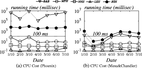
Running time on Mobile phone- Yelp

References
Gowalla dataset. http://snap.stanford.edu/data/loc-gowalla.html
Yelp dataset. http://www.yelp.com/dataset_challenge/
Agrawal R, Srikant R (1994) Fast algorithms for mining association rules in large databases. VLDB ’94. San Francisco, pp 487–499. http://dl.acm.org/citation.cfm?id=645920.672836
Alfarrarjeh A, Emrich T, Shahabi C (2014) Scalable spatial crowdsourcing: A study of distributed algorithms. MDM ’15
Alt F, Shirazi AS, Schmidt A, Kramer U, Nawaz Z (2010) Location-based crowdsourcing: extending crowdsourcing to the real world. NordiCHI ’10. NY, pp 13–22. doi:10.1145/1868914.1868921
Bozzon A, Brambilla M, Ceri S, Mazza D (2013) Exploratory search framework for web data sources. VLDB J 22(5):641–663
Bulut M, Yilmaz Y, Demirbas M (2011) Crowdsourcing location-based queries. In: PERCOM workshops. doi:10.1109/PERCOMW.2011.5766944, pp 513–518
Chen C, Cheng SF, Gunawan A, Misra A, Dasgupta K, Chander D (2014) Traccs: a framework for trajectory-aware coordinated urban crowd-sourcing. In: 2nd AAAI conference on human computation and crowdsourcing
Chen C, Cheng SF, Misra A, Lau HC (2015) Multi-agent task assignment for mobile crowdsourcing under trajectory uncertainties. In: Proceedings of the 2015 International Conference on Autonomous Agents and Multiagent Systems, AAMAS ’15. http://dl.acm.org/citation.cfm?id=2772879.2773400. International Foundation for Autonomous Agents and Multiagent Systems, Richland, pp 1715–1716
Chen Z, Fu R, Zhao Z, Liu Z, Xia L, Chen L, Cheng P, Cao CC, Tong Y, Zhang CJ (2014) gmission: A general spatial crowdsourcing platform. PVLDB
Dabrowski JR, Munson EV (2001) Is 100 milliseconds too fast?. In: CHI ’01 extended abstracts on human factors in computing systems, CHI EA ’01, pp 317–318
Demartini G, Difallah DE, Cudré-Mauroux P (2013) Large-scale linked data integration using probabilistic reasoning and crowdsourcing. VLDB J 22(5):665–687
Deng D, Shahabi C, Demiryurek U (2013) Maximizing the number of worker’s self-selected tasks in spatial crowdsourcing. In: SIGSPATIAL’13. doi:10.1145/2525314.2525370, pp 314–323
Deng D, Shahabi C, Zhu L (2015) Task matching and scheduling for multiple workers in spatial crowdsourcing. In: SIGSPATIAL’15. doi:10.1145/2525314.2525370
Doan A, Ramakrishnan R, Halevy AY (2011) Crowdsourcing systems on the world-wide web. Commun ACM 54(4):86–96
Franklin MJ, Kossmann D, Kraska T, Ramesh S, Xin R (2011) Crowddb: answering queries with crowdsourcing. SIGMOD ’11. NY, pp 61–72
Grady C, Lease M (2010) Crowdsourcing document relevance assessment with mechanical turk. NAACL HLT ’10. PA, pp 172–179
Guo S, Parameswaran A, Garcia-Molina H (2012) So who won?: dynamic max discovery with the crowd. SIGMOD ’12. NY, pp 385–396
Hull B, Bychkovsky V, Zhang Y, Chen K, Goraczko M, Miu A, Shih E, Balakrishnan H, Madden S (2006) Cartel: a distributed mobile sensor computing system. SenSys ’06. NY, pp 125–138. doi:10.1145/1182807.1182821
Kantor MG, Rosenwein MB (1992) The orienteering problem with time windows. J Oper Res Soc 629–635
Kazemi L, Shahabi C A privacy-aware framework for participatory sensing. SIGKDD Explor ’11 13(1):43–51
Kazemi L, Shahabi C (2012) Geocrowd: enabling query answering with spatial crowdsourcing. In: SIGSPATIAL ’12. doi:10.1145/2424321.2424346. NY, pp 189–198
Kazemi L, Shahabi C, Chen L (2013) Geotrucrowd: Trustworthy query answering with spatial crowdsourcing. In: SIGSPATIAL’13, pp 304–313
Layla Pournajaf LX, Sunderam V (2014) Dynamic data driven crowd sensing task assignment. Proc Comput Sci 29:1314–1323. doi:10.1016/j.procs.2014.05.118. http://www.sciencedirect.com/science/article/pii/S1877050914002956. 2014 International Conference on Computational Science
Lee SM, Asllani AA (2004) Job scheduling with dual criteria and sequence-dependent setups: mathematical versus genetic programming. Omega 32 (2):145–153. doi:10.1016/j.omega.2003.10.001. http://www.sciencedirect.com/science/article/pii/S0305048303001324
Li F, Cheng D, Hadjieleftheriou M, Kollios G, Teng SH (2005) On trip planning queries in spatial databases. SSTD’05. Berlin, pp 273–290. doi:10.1007/11535331_16
Li Y, Deng D, Demiryurek U, Shahabi C, Ravada S (2015) Towards fast and accurate solutions to vehicle routing in a large-scale and dynamic environment. In: SSTD, vol 9239, pp 119–136
Li Y, Yiu ML, Xu W (2015) Oriented online route recommendation for spatial crowdsourcing task workers. In: Advances in spatial and temporal databases. Springer, pp 137–156
Marcus A, Wu E, Madden S, Miller RC (2011) Crowdsourced databases: query processing with people. In: CIDR, pp 211–214
Mohan P, Padmanabhan VN, Ramjee R (2008) Nericell: rich monitoring of road and traffic conditions using mobile smartphones. SenSys ’08. NY, pp 323–336. doi:10.1145/1460412.1460444
Moore JM (1968) An n job, one machine sequencing algorithm for minimizing the number of late jobs. Manag Sci 15(1):102–109. http://www.jstor.org/stable/2628449
Musthag M, Ganesan D (2013) Labor dynamics in a mobile micro-task market. In: Proceedings of the SIGCHI conference on human factors in computing systems. ACM, pp 641–650
Pan B, Zheng Y, Wilkie D, Shahabi C (2013) Crowd sensing of traffic anomalies based on human mobility and social media. In: SIGSPATIAL’13. doi:10.1145/2525314.2525343, pp 334–343
Papadimitriou CH (1977) The euclidean travelling salesman problem is np-complete. Theor Comput Sci 4(3):237–244. doi:10.1016/0304-3975(77)90012-3. http://www.sciencedirect.com/science/article/pii/0304397577900123
Pournajaf L, Xiong L, Sunderam V, Goryczka S (2014) Spatial task assignment for crowd sensing with cloaked locations. In: Proceedings of the 2014 IEEE 15th international conference on mobile data management, MDM ’14. doi:10.1109/MDM.2014.15, vol 1. IEEE Computer Society, Washington, DC, pp 73–82
Sharifzadeh M, Kolahdouzan M, Shahabi C (2008) The optimal sequenced route query. VLDB J 17(4):765–787. doi:10.1007/s00778-006-0038-6
Snow R, O’Connor B, Jurafsky D, Ng AY (2008) Cheap and fast—but is it good?: evaluating non-expert annotations for natural language tasks. EMNLP ’08. PA, pp 254–263
Teodoro R, Ozturk P, Naaman M, Mason W, Lindqvist J (2014) The motivations and experiences of the on-demand mobile workforce. In: Proceedings of the 17th ACM conference on computer supported cooperative work & social computing. ACM, pp 236–247
Terrovitis M, Bakiras S, Papadias D, Mouratidis K (2005) Constrained shortest path computation. In: SSTD’05. doi:10.1007/11535331_11, vol 3633, pp 181–199
To H, Ghinita G, Shahabi C (2014) A framework for protecting worker location privacy in spatial crowdsourcing. Proc VLDB Endowment 7(10)
To H, Shahabi C, Kazemi L (2015) A server-assigned spatial crowdsourcing framework. ACM Trans Spatial Algorithms Syst 1(1):2:1–2:28. doi:10.1145/2729713
Wang Y, Huang Y, Louis C (2013) Towards a framework for privacy-aware mobile crowdsourcing. In: International conference on social computing (SocialCom), 2013. IEEE, pp 454–459
Yan T, Kumar V, Ganesan D (2010) Crowdsearch: exploiting crowds for accurate real-time image search on mobile phones. MobiSys ’10. NY, pp 77–90
Yang K, Zhang K, Ren J, Shen X (2015) Security and privacy in mobile crowdsourcing networks: challenges and opportunities. IEEE Commun Mag 53(8):75–81. doi:10.1109/MCOM.2015.7180511
Zenonos A, Stein S, Jennings NR (2015) Coordinating measurements for air pollution monitoring in participatory sensing settings. In: Proceedings of the 2015 international conference on autonomous agents and multiagent systems. International Foundation for Autonomous Agents and Multiagent Systems, pp 493–501
Acknowledgments
This research has been funded in part by NSF grants IIS-1115153 and IIS-1320149, a contract with Los Angeles Metropolitan Transportation Authority (LA Metro), the USC Integrated Media Systems Center (IMSC), HP Labs and unrestricted cash gifts from Google, Northrop Grumman, Microsoft and Oracle. Any opinions, findings, and conclusions or recommendations expressed in this material are those of the author(s) and do not necessarily reflect the views of any of the sponsors such as the National Science Foundation or LA Metro.
Author information
Authors and Affiliations
Corresponding author
Additional information
A preliminary version of this work [13] appeared in ACM SIGSPATIAL GIS 2013.
Rights and permissions
About this article

Cite this article
Deng, D., Shahabi, C., Demiryurek, U. et al. Task selection in spatial crowdsourcing from worker’s perspective. Geoinformatica 20, 529–568 (2016). https://doi.org/10.1007/s10707-016-0251-4
Received:
Revised:
Accepted:
Published:
Issue Date:
DOI: https://doi.org/10.1007/s10707-016-0251-4