
Abstract
In nonlinear structural response time history analysis, defining a target spectrum and selecting a suitable set of seismic ground motion records are of paramount importance. Commonly used target spectra include the Uniform Hazard Spectrum (UHS) and the Conditional (Mean) Spectrum (CMS or CS). The CMS (CS) mitigates the limitations of UHS, which are characterized as “overly conservative” and having an “unrealistic spectral shape”. It has been employed as a target spectrum in recent years. However, CMS only considers the fundamental period T1 of the structure while ignoring the effects of higher modes on the structure. For tall buildings and irregular structures, CMS may not provide a complete solution. To address this issue, this study proposes a modal conditional mean spectrum (MCMS) on the foundation of CMS to account for the effects of higher modes. MCMS is constructed by employing modal participation mass-weighted averaging, the value of the CMS is enhanced for short periods, while the long-period portion remains unchanged. Subsequently, two high-rise case study structures (symmetric and asymmetric) are designed, and nonlinear structural response time history analyses are conducted using MCMS, CMS (T1), and UHS as target spectra. Through a compare of four engineering demand parameters: Peak Floor Acceleration (PFA), Peak Floor Velocity (PFV), Peak Floor Displacement (PFD), and Maximum Interstory Drift Ratio (IDR), the results indicate that the structural responses for UHS are 1.3–1.9 times greater than those for CMS, and the structural responses for MCMS exceed those for CMS by 6–11%.
1 Introduction
Selection and scaling of earthquake ground motion are associated with nonlinear structural response time-history dynamic analysis in performance‐based seismic evaluation of earthquake engineering (Goulet et al. 2007). The basic steps for ground motion selection and scaling include the following: (1) Develop an appropriate target spectrum. (2) Selection and scaling a suitable set of earthquake ground motion records in accordance with the target spectrum. A smart target spectrum can be used to minimize approximation effects due to combining site hazard and structural response prediction through an “aimed” set of earthquake ground motion records. Such a target spectrum could be a uniform hazard spectrum (UHS) (McGuire 1995), design response spectrum (DRS), conditional mean spectrum (CMS) (Baker 2011), conditional spectrum (CS) in which both the mean and deviation are considered (Jayaram et al. 2011a, b), and Eta-based conditional mean spectrum (E-CMS) (Mousavi et al. 2011). A UHS is developed by carrying out probabilistic seismic hazard analysis (PSHA) calculations, and any point on it represents that every spectral acceleration value has an equal rate of being exceeded. However, it should be clear that a UHS is essentially an envelope response spectral acceleration of all earthquakes at a site (Bommer et al. 2000), rather than originating from an actual earthquake. In different periods, each spectral acceleration value may come from different controlling earthquake scenarios. However, for the specific structure of a site, the spectral acceleration value cannot be reached using the UHS at all periods (Baker and Cornell 2005), leading to a conservative structural response calculated according to the UHS, which is not conducive to the accurate evaluation of seismic performance of a structure (Naeim and Le 1995; Reiter 1990). A DRS is statistically averaged from the acceleration response spectrum of many earthquake ground motion records and formulated to several straight lines or curves (such as the DRS in the ASCE/SEI 7-10 (2010), Eurocode 8 (2004), and Chinese Code (CCSDB 2010)). Thus, a DRS is essentially a UHS abstracted with empirical formulas.
To overcome the limitations of the “overly conservative” and “unrealistic spectral shape” of a UHS or DRS, Baker and Cornell (2008), Baker (2011) proposed the CMS as an alternative target spectrum by considering the spectral shape parameter ε. From the definition of CMS, it can be seen that the CMS matches the UHS at a single conditioning period T*. In a period far from T* (T < T* or T > T*), the divergence between the UHS and CMS gradually increases, eliminating the “conservatism” of the UHS (Baker and Cornell 2006). Furthermore, the spectral shape of the CMS is closer to the response spectrum of a ground motion record, which can better reflect the characteristics of the actual ground motion. Haselton et al. (2008) analyzed a reinforced concrete (RC) frame structure considering the spectral shape parameter ε to compare the CMS and UHS, and the results showed that selecting ground motions without considering ε increases the structural response by 30–60%. Eads et al. (2016) investigated various parameters for characterizing spectral shape measurements, proposed and evaluated a metric for quantifying the spectral shape called SaRatio, and studied how they are potentially linked to ground motion records that induce collapse in a given structure. The results indicate that SaRatio generally provides better predictions of collapse intensity compared to other spectral shape indicators.
To estimate the probability distribution of the structural response under a certain earthquake hazard level, the conditional standard deviation should be considered in addition to the CMS. Jayaram et al. (2011a, b) and Lin et al. (2013a, b, c) proposed that the conditional spectrum (CS) simultaneously matches the mean and deviation of the target spectrum. Lin et al. (2013a, b, c) studied the mean value and distribution of the CMS and CS spectral response under both risk-based assessments and intensity-based assessments, and the results proved that the CMS yielded similar median estimates of structural response compared to CS but exhibited lower dispersion due to missed variability. In addition, the results showed that the influence of the selection of the conditioning period for the CS on structural response estimates is more sensitive in an intensity-based assessment than in a risk-based assessment. Haselton et al. (2009) compared and analyzed 14 ground motion selection and scaling schemes for 4 kinds of RC frame and shear wall structures, showing that the CMS and CS have higher estimation accuracy for predicting the median values of interstory drift ratio of buildings. Fox and Sullivan (2016) proposed a simplified seismic assessment procedure of RC wall structures based on the CS to incorporate record-to-record variability. Hashash et al. (2015) took a site-specific location near a Mississippi River crossing in the central United States as an example to construct the corresponding CMS, which proved its rationality from the perspective of the actual site response. Mousavi et al. (2012) proposed an E-CMS method by considering the influence of the peak velocity PGV (η, a new indicator of the elastic spectral shape) on the basis of the CMS. The results show that the correlation of the CMS with period and ductility is more significant when η is considered. In a study by Azarbakht et al. (2015), the E-CMS was employed as the target spectrum for record selection. The analysis of a group of multi-degree-of-freedom systems indicated that, based on the newly introduced η index, deviations can be reduced, leading to a higher average annual collapse frequency and increased reliability. Particularly at elevated hazard levels, or when dealing with low natural periods or significant high-mode effects, the reduction in deviations becomes more pronounced. In addition, E-CMS is joined to the PSHA in an explicit way, which is also generally accepted. In another work by Mohandesi et al. (2019), utilizing a simplified linear seismic source, the seismic hazard decomposition based on the η index was explored. The E-CMS was applied across different hazard levels for the purpose of selecting ground motion records. Subsequently, an analysis was conducted on a three-story building using these selected records. Shantz (2006) constructed an inelastic displacement surface (IDS) spectrum based on the CMS. The IDS spectrum is a three-dimensional surface spectrum with period T as the x coordinate, the displacement ductility coefficient μ as the y coordinate, and the maximum displacement reaction as the z coordinate to predict the nonlinear reaction of a structure. In addition, the aftershock after the main earthquake will increase the damage to a structure, resulting in a cumulative damage effect. Zhu et al. (2017) constructed the CMS considering the main shock‐aftershock ground motion sequences.
The CMS (CS) has been employed worldwide, and there are many practical application cases of constructing a local CMS in many countries. For example, Vacareanu et al. (2014) constructed the CMS of Bucharest, and Daneshvar et al. (2015) constructed the CMS of Eastern Canada. It has also been used in the evaluation of the seismic performance of buildings (Daneshvar et al. 2014) and dams (Bernier et al. 2016). Ji et al. (2017) first researched the correlation coefficients of spectral accelerations used to generate a CMS based on ground motion records from 2007 to 2014 in China. Then, implementation and specific-case studies of the CMS and CS based on seismic safety evaluation in China were given (Ji et al. 2018). Based on ArcGIS, Li (2016) completed seismic hazard disaggregation in the Xi 'an area in China and obtained the UHS and CMS of the area. In addition, several kinds of application software have been developed based on the CMS, such as the online ground motions selection database tool developed by PEER (https://ngawest2.berkeley.edu/), the Conditional Spectrum Ground Motions Selection (CSGMS) software developed by Baker and Lee (2018), the QuakeManager software developed by Mahmoud (2008), and the Design Ground Motion Library (DGML) developed by Wang et al. (2015).
According to the aforementioned studies, a CMS method considering the spectral shape parameters has received increasing attention and recognition by earthquake engineering scholars and has also been accepted as a more reasonable target spectrum recently. However, with the deepening of the research, this method has encountered the following two bottlenecks. First, the CMS only selects only one conditional period (usually the first mode of the structure corresponding to the first period T1), ignoring the influence of the high-order vibration mode (other periods) on the structure. This is acceptable for low-rise structures controlled by the basic period T1, but for high-rise structures (especially super high-rise buildings and irregular buildings), the use of the CMS will introduce new problems. According to the theory of modal analysis of structural dynamics, the response of a multi-degree-of-freedom (MDOF) structure can be regarded as the result of the superposition of multiple modes, and the influence of each mode on the whole structure can be measured by the modal participation mass ratio. As the number of degrees of freedom (DOFs) of a structure increases or the irregularity increases, the participating mass ratio of the first mode of the structure will decrease, and the participating mass ratio of a higher-order mode will become larger, which may cause the basic period T1 to not be controlled. Thus, for high-rise buildings (super high-rise and irregular) or bidirectional ground motion inputs that need to consider the multimode effect (Bradley 2012a, b), it is often necessary to consider multiple periodical points, and the CMS as the target spectrum has obvious shortcomings. This problem is an important bottleneck limiting the generalization and wide application of the CMS. Second, an acceleration response spectrum is essentially the response value of an elastic one-degree-of-freedom system, so it cannot reflect the duration and energy accumulation effects of ground motion well. Bradley (2010, 2012a, b) proposed a generalized conditional mean spectrum method (GCMS) to solve these two problems so that the selected ground motion could meet multiple parameters sets (including energy, duration, intensity, amplitude, etc.) at the same time. Kwong and Chopra (2017) proposed a simplified generalized conditional mean spectrum algorithm for structures that may be affected by two modes, which can match two conditional periods at the same time without the need to separate seismic hazard disaggregation and CMS calculation. In practical applications, it was found that although the above latest research results provide two feasible ways to construct a generalized CMS, there are still some problems before practical application. Bradley's GCMS approach is more mathematically focused, but lacks a direct link to structural properties. Kwong and Chopra's simplified generalized CMS method can only consider two conditional periods, both of which should not be too far apart.
Su et al. (2016) introduced an innovative seismic intensity metric that incorporates higher-order cyclic vibration modes into the comprehensive assessment of mass coefficients and spectral acceleration values. Research has demonstrated a substantial and meaningful correlation between this metric and structural demand parameters. Additionally, Zhang et al. (2018, 2019) proposed a novel matching technique that accounts for the influence of higher-order vibration modes. By utilizing vibration mode participation coefficients as weights across different periods, this method effectively reduces the discreteness of computational outcomes. In summary, the aforementioned studies approach the consideration of higher-order vibration modes from various angles in time-history analysis, employing vibration mode participation coefficients to quantify the extent of their impact. Therefore, based on modal analysis theory and the CMS, this paper proposes a modal conditional mean spectrum (MCMS) considering the influence of higher-order modes. Based on the idea of mode superposition in modal analysis, this method considers the influence of higher-order mode shapes by weighted (measured using the modal participation mass ratio) averaging the conditional mean spectrum under each period of the structure. Moreover, this method considers that the multi-conditional period is from the structure itself, so it has a clear physical meaning. Then, two typical high-rise structures (symmetric and asymmetric structures) were designed, and nonlinear structural response time-history analysis was constructed for the two structures using the new MCMS. The results were compared with the traditional CMS(T1) (single conditional period T1) and UHS, which proved the rationality of considering the influence of higher-order mode effects.
2 Proposed modal conditional mean spectrum
The construction process of MCMS is illustrated in the flowchart shown in Fig. 1. The calculation procedure can be broken down into eight distinct steps:

MCMS construction process
-
(1)
PSHA to obtain UHS
Firstly, we need to conduct a PSHA for the given site to obtain the UHS at different exceedance probabilities. Typically, UHS values are selected for exceedance probabilities of 2% in 50 years, 10% in 50 years, and 63% in 50 years, corresponding to return periods of 2475 years, 474 years, and 50 years, respectively.
-
(2)
Modal analysis
For the given structure, a modal analysis is performed. Unlike traditional CMS that only requires the primary periods of the structure, in the MCMS approach, we need to obtain the periods of all vibration modes Ti and their corresponding mode participation mass ratios \(\lambda_{i}\). Based on the definition of \(\lambda\), the sum of the masses participating in all modes is equal to the total mass, i.e.,
$$\sum\limits_{i = 1}^{N} {\lambda_{i} = 1}$$(1)This value reflects the relative contribution of each mode to the structural dynamic response. Therefore, it is a constant ranging from 0 to 1. As the mode order increases, the value continuously decreases, indicating that higher mode vibrations contribute less to the structural dynamic response. This step can be obtained through finite element analysis software.
-
(3)
Determine a target Sa and deaggregation, given T
Before starting the calculation, we need to determine a target Sa (Spectral Acceleration) value at a specific period of interest. This period of interest can be selected from the modal analysis results, which provide the periods of all vibration modes. The target Sa value, Sa(Ti), can be obtained from the UHS at the corresponding period Ti.
Additionally, we need to determine the seismic magnitude (M), distance (R), and epsilon (\(\varepsilon\)) values associated with the target Sa(Ti). The M-R (Magnitude–Distance) values can be chosen from the mean values obtained from deaggregation, where deaggregation is a process that decouples seismic hazard analysis. It involves using Bayesian principles to infer the contribution proportions of earthquake parameter combinations that simultaneously satisfy seismic activity and spatial compatibility of potential seismic sources based on the results of the site hazard analysis.
-
(4)
Given M and R, calculate the mean and standard deviation of the response spectrum.
Next, we compute the mean and standard deviation of the logarithmic spectrum acceleration values (\(\mu \ln Sa(M,R,T_{i} )\) and \(\sigma_{\ln Sa} (T_{i} )\)) across all periods, for the given target values of M, R. These terms can be calculated using existing ground motion models, and there are online computational tools available to assist in obtaining these values (for example, http://www.opensha.org and http://peer.berkeley.edu/products/rep_nga_models.html).
$$\varepsilon (T) = \frac{{\ln Sa(T) - \mu_{\ln Sa(M,R,T)} }}{{\sigma_{\ln Sa(T)} }}$$(2) -
(5)
Given ε(Ti), calculate ε at all other periods Tk.
The conditional mean at other period points can be regarded as the product of coefficient \(\varepsilon (T_{i} )\) multiplied by the correlation coefficient between the two periods' \(\varepsilon\), as shown in Eq. 3.
$$\mu \varepsilon (T_{k} )|\varepsilon (T_{i} ) = \rho (T_{k} ,T_{i} )\varepsilon (T_{i} )$$(3)where \(\mu \varepsilon (T_{k} )|\varepsilon (T_{i} )\) represents the mean of \(\varepsilon (T_{k} )\) under the given condition \(\varepsilon (T_{i} )\), and \(\rho (T_{k} ,T_{i} )\) denotes the correlation coefficient between two periods. A simplified prediction formula for correlation coefficients applicable to the US was provided by Baker (2011). The correlation coefficient for spectral acceleration in China can be referenced from Ji et al. (2017). This correlation coefficient will be utilized in the subsequent numerical validations in this article.
-
(6)
Calculate CMS(Ti).
CMS can now be calculated using the mean and standard deviation from step 4, along with the conditional mean ε from step 5. By substituting Eq. 3 into Eq. 2, we obtain the corresponding conditional mean of \(\ln Sa(T)\) under the given condition \(\ln Sa(T_{i} )\). This is shown in Eq. 4:
$$\mu \ln Sa(T_{k} )|\ln Sa(T_{i} ) = \mu \ln Sa(M,R,T_{k} ) + \rho (T_{k} ,T_{i} )\varepsilon (T_{i} )\sigma_{\ln Sa} (T_{k} )$$(4)where \(\mu \ln Sa(M,R,T)\) and \(\sigma_{\ln Sa} (T)\) are defined as presented, and \(\rho (T_{k} ,T_{i} )\) can be computed from Eq. 5. M, R, \(\varepsilon (T_{i} )\) are obtained from the step 4 of deaggregation.
-
(7)
Calculate the weighted values of CMS.
Utilizing the natural periods as the periods of interest (T*), repeat the aforementioned steps 3–6. This will yield conditional mean spectra CMS(T1), CMS(T2), … CMS(Tn) corresponding to each natural period. Assuming the first four natural periods of the structure are 3s, 1s, 0.5s, and 0.4s, their corresponding CMS values are illustrated in Fig. 2. Finally, employing the participation mass ratios \(\lambda_{i}\) associated with each period's mode shape as weights, perform a weighted aggregation of CMS(Ti), resulting in a modal weighted conditional mean spectrum (MWCMS) that accounts for higher-order mode shapes, as depicted in Eq. 5.
$$Sa_{MWCMS} (T) = \sum\limits_{i = 1}^{N} {\lambda_{i} } Sa(T_{i} )$$(5)Fig. 2 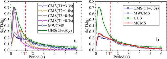
Comparison of Target Spectra for Case 1 in this study
The value of SaMWCMS(T) represents the Sa of MWCMS, and Sa(Ti) represents the value of the CMS corresponding to the period Ti. By performing a weighted average of the CMS values for all modes of the structure, theoretically, an optimal result can be obtained. Since the contribution of higher-order modes decreases with increasing mode order (as λ decreases), in practical applications, modes of exceptionally high order can be disregarded to reduce computational effort. According to the Chinese Code (CCSDB 2010) regulations for modal superposition methods, the first j terms of the nth mode are considered, ensuring that the participation mass ratio exceeds 90% of the total mass, i.e., \(\sum\nolimits_{i = 1}^{j} {\lambda_{i} } > 90\%\). This leads to a normalized and simplified MWCMS, as shown in Eq. 6.
$$Sa_{MWCMS} (T) = \frac{{\sum\nolimits_{i = 1}^{j} {\lambda_{i} } Sa(T_{i} )}}{{\sum\nolimits_{i = 1}^{j} {\lambda_{i} } }}$$(6)The construction of target spectra for Case 1 in this study is presented ahead in this section. In this Case, the sum of \(\lambda\) for the first four modes alone reaches 90%, with corresponding periods of 3.4 s, 1.0 s, 0.5 s, and 0.3 s. The comparisons of CMSs for each mode, UHS, MWCMS, are shown in Fig. 2a.
-
(8)
Construction of MCMS
From Fig. 2a, it can be observed that MWCMS intersects with CMS (T1) at a point labeled as T". To the left of T", due to the consideration of the influence of higher-order structural modes and the inherent characteristics of the CMS spectral shape, the Sa values of MWCMS are greater than those of CMS (T1). Conversely, to the right of T", because the higher-order periods of CMS exhibit faster attenuation in the long-period range, the resulting Sa of MWCMS are lower than those of CMS (T1). To account for the influence of higher-order structural modes without diluting the effects of nonlinearity, this study combines the characteristics of MWCMS and CMS (T1), defining the Sa of MCMS as Eq. 7
$$Sa_{MCMS} (T) = \left\{ {\begin{array}{*{20}c} {Sa_{MWCMS} (T)} & {(T < T^{\prime\prime})} \\ {Sa_{{CMS(T_{1} )}} (T)} & {(T > T^{\prime\prime})} \\ \end{array} } \right.$$(7)

On the left side of T", the MCMS Sa is equal to the MWCMS. On the right side of T", the Sa of MCMS is equal to the CMS (T1). As the MWCMS intersects with CMS (T1) at T", MCMS maintains continuity at T", as illustrated in Fig. 2b.
3 Case study: structures and target spectra
3.1 Case structure design and modeling
In this study, two 30-story steel frame-center braced structures (symmetric and asymmetric 2D structures) are designed as Cases to verify the MCMS theory, and the design process follows the rules of the Chinese Code CCSDB (2010) and CSDSS (2017). Both case structures are located in Ya'an City (latitude = 29.795° N and longitude = 102.846° E), Sichuan Province, China, with a seismic design intensity of 7 degrees (the design the peak ground acceleration value of 0.15 g) and a site category of Class II (equivalent shear wave velocity to 30 m depth is 360 m/s). The design value of the dead load of the floor and roof is 3.5 KN/m2, and the design value of the equivalent uniform live load is 2 KN/m2. The frame beams and columns and braced components are selected according to the Chinese Code (CHRCSS 2017) with hot-rolled wide flange H-beams (HW), and the steel strength is Q345.
The frame of Case 1 has three spans. Each span is 6000 mm, and the story height is 3000 mm. A set of chevron central braces is set in the middle span of the frame plane, and the angle between the braces and the beam axis is 45°. The elevation arrangement of the structure is shown in Fig. 3a. The frame of Case 2 has four spans. Each span is 9000 mm, and the story height is 3600 mm. In the frame plane, the fourth span is retracted at the 10th floor, the third span is retracted at the 15th floor, and the first span is retracted at the 22nd floor. A set of chevron central bracing is arranged in the area of floors 1–26 of the second span, with an angle of 38.7° between the bracing and the beam axis. The elevation arrangement of the structure is shown in Fig. 3b. The selection of member sectional information for the two case structures is shown in Table 1.

Elevations of the two case structures, a Case 1, b Case 2 (unit: mm)
The finite element analysis of the structure was performed using OpenSees software, with the steel frame using nonlinear beam-column elements (Pacone et al. 1996) and the braced component using truss elements, which can release of the moment freedom to consider pin connection. The cross-section is discretized into a fiber section, and the corresponding constitutive model of steel material is assigned to the fibers. The Steel01 model is used for the steel material. Steel01 is a kinematic strain-hardening model, the most important feature of which is that it considers the Bauschinger effect and the degradation of strength and stiffness.
3.2 Modal analysis results
The modal analysis of the two case structures was performed, and the periods and their modal participating mass ratios were obtained as shown in Table 2. Eigen-value periodicity is being utilized in this study, and for concrete structures, we consider the period during their uncracked elastic phase. According to the previous section, the selection of the mode orders was determined with the modal participating mass ratios being greater than 90%, so the first four orders were considered for both cases.
3.3 Creation of the UHS, CMS and MCMS
This study will reference the results of the China Sichuan Ya'an UHS and CMS constructed by (Ji 2018). In the site-specific PSHA analysis, two dominant seismic zones in the vicinity were considered: Longmenshan seismic zone and Xianshuihe-Dongdian seismic zone, comprising nine potential seismic sources. Their distribution can be seen in Fig. 2 of Ji et al. (2018). The HUO89 Ground Motion Prediction Equation (GMPE), suitable for application in China, is adopted. The obtained UHS for 63%, 10%, and 2% exceedance probabilities in 50 years are shown in Fig. 4. Following the disaggregation method (McGuire 1995) for target earthquakes, which involves deducing the contribution ratios of different earthquake parameter combinations from the results of PSHA, the 3D results for the first four periods of the designated earthquakes are obtained. Since the periods for Case 1 and Case 2 are similar, and their 3D results are also comparable, we only present the results for Case 1, as depicted in Fig. 5. Subsequently, in the calculations, only the dominant scenarios (peak scenarios) are employed, similar to the approach by Ebrahimian et al. (2012). The decomposition results of the dominant scenarios for both cases are presented in Table 3. For further detailed descriptions that have not been covered here, please refer to the mentioned reference.

UHS for the site with the 63, 10, and 2% exceedance probability in 50-year

Results of the PSHA disaggregation results given the UHS with 2% probability of exceedance in 50 years of Case 1, a Sa (T1 = 3.3 s), b Sa (T2 = 1.0 s), c Sa (T3 = 0.5 s), d Sa (T4 = 0.3 s)
The CMS at each interesting period for the two cases was generated according to Eq. 4, and the values of the MCMS of the two cases were further calculated according to Eqs. 6 and 7. The final obtained target spectra for Case 2 are presented in Fig. 6, encompassing the UHS with a 2% exceedance probability in 50 years, CMS corresponding to various periods, WACMS, and MCMS. It should be noted that the target spectra results for Case 1 have already been shown in Fig. 2 of Sect. 2. The values of T'' for Case 1 and Case 2 are located around 1.3s and 1.35s, respectively.

Comparison of Target Spectra for Case 2
Similar results were found for the hazard level with a 10% exceedance probability and a 63% exceedance probability in 50 years. Given the limited length of the article, we only provide the results CMS and MCMS for the hazard level with the 2% exceedance probability in 50-year.
3.4 Selection and scaling of ground motion records
In this study, the UHS, the CMS(T1), and the MCMS with 63%, 10%, 2% exceedance probability in 50 years of the two cases are used as the target spectra. Due to space constraints, similarly in this section of the records matching, results are given for only 2% exceedance probability in 50 years. The database of matched ground motion records is from PEER NGA-west2 (https://ngawest2.berkeley.edu/) with a magnitude interval of (5.5, 8.5) and a source-to-site distance interval of (80 km, 95 km), The matching period range is (0.3 s, 2T1), where T1 represents the fundamental period of structures.
In the context of spectra matching, according to Chinese code (CCSDB 2010), it is required that the records average response spectra should deviate from the target spectrum by no more than 20% at the fundamental period. This differs from the provisions in other countries' codes. For instance, ASCE/SEI 7-10 specifies that the average response spectrum should not be less than the target spectrum, while Eurocode 8 (Part 1) stipulates that the average response spectrum should not be lower than 90% of the target spectrum. In this study, adhering to Chinese code, we have employed a simple and effective weighted least-squares error (WLSE) method to quantify the agreement of matched ground motion records and the target spectrum as described in Zhang et al. (2019). The equation of WLSE is shown in Eq. 8, where \(w(T_{i} )\) is the weighting factors, \(Sa(T_{i} )\) and \(Sa(T_{i} )^{target}\) are the acceleration response spectrum values of the ground motion records and the target spectrum, respectively. In this study, we do not consider the effect of weighting factors, i.e., we take all of \(w(T_{i} )\) = 1.
The 30 records with the smallest WLSE values were selected from the database for each target spectrum, and information of five sets (CMS for Case 1, MCMS for Case 1, CMS for Case 2, MCMS for Case 2, and UHS for both Case 1 and 2) of ground motion records were provided in Appendix Table 4, and the spectrum shape is shown in Fig. 7. The five sets of ground motion records were input into the above OpenSees model for structural nonlinear time-history analysis.

The spectra of the selected records: a CMS for Case 1, b MCMS for Case 1, c CMS for Case 2, d MCMS for Case 2, and e UHS
3.5 Analysis of ground motion records response spectra
Two sets of seismic records were matched using three target spectra, resulting in 30 response spectra. Figure 8 shows a comparison of the mean acceleration response spectra, velocity response spectra, and displacement response spectra for the selected records, with a common 5% damping ratio used in the response spectrum calculation.

Comparison of the mean values of the three best-matched response spectra (2%/50 y)
Figure 8a and b display the acceleration response spectra for the two cases. It can be observed that MCMS and CMS closely coincide and overlap in the long-period range (T > 1.5 s), while in the short-period range (T < 1.5s), MCMS consistently yields higher results compared to CMS. This trend aligns with the behavior of the target spectra, indicating that the seismic record matching methods effectively capture the spectral characteristics of the target spectra and highlight the differences between different target spectra.
Figure 8c and d show the velocity response spectra for the two cases. The overall trend of the UHS is significantly higher than CMS and MCMS, as expected. MCMS consistently yields higher velocity spectra values compared to CMS across all periods. The velocity response spectra are particularly sensitive in the mid-period range, resulting in peaks in that region. MCMS's velocity response spectra peak around 1.8s is approximately 10% higher than CMS's, while UHS's velocity response spectra are about 60% higher than CMS and MCMS.
Figure 8e and f display the displacement response spectra for the two cases. The displacement response spectra exhibit more variation in the long-period range, which is in accordance with structural dynamics knowledge. Similar to the velocity response spectra comparison, MCMS consistently yields higher spectral values compared to CMS across all periods. At the main period, MCMS's displacement spectra values are about 6% higher (Case 1) and 9% higher (Case 2) than CMS's.
4 Results and discussions of case study
In this section, we will discuss the results of time history analysis, which involve three hazard levels (2%/50 years, 10%/50 years, and 63%/50 years), four structural response demands (PFA, PFV, PFD, IDR), and the selection of 5 and 30 seismic records. Due to the significant variability and uncertainty among seismic records, in the analysis of results, it is common practice to use the average of a set of records to represent the response corresponding to the target spectrum. Therefore, Due to space constraints, we will only provide the mean results for each Case.
Figures 9, 10, 11 and 12 present the average values of PFA, PFV, PFD, and IDR obtained from time history analyses using different sets of records at various hazard levels for the two cases. Different target spectra are represented by different colors in the figures. Solid symbols indicate the mean values from 30 records, while hollow symbols represent the mean values from 5 best matched records.
From the overall results of the four sets of structure response, it can be observed that the general trends for both cases remain relatively consistent across the three hazard levels, with variations primarily seen in numerical values. For the same target spectrum, the structure response might exhibit slight variations at specific floors due to the different number of selected records. Overall, it is evident that the UHS yields significantly higher values compared to CMS and MCMS results, which is expected. Additionally, considering the influence of higher-mode effects, MCMS produces larger spectral values than CMS in the short-period range. As a result, all four sets of structure response calculated using MCMS records selection are higher than those obtained with CMS records selection.
4.1 Peak floor acceleration (PFA) results
Figure 9 displays the analysis results of PFA. In both cases, PFA sharply increases with the elevation of floors and reaches a stable value around the 10th floor. Beyond the 25th floor, due to the effect of the whip mode, PFA dramatically increases again, and its peak value occurs at the top floor. Comparing the maximum PFA values at the top floor, Case 1 with MCMS is 11.7% and 9.9% higher (for 5 records and 30 records, respectively) than CMS, while Case 2 with MCMS is 13.4% and 14.3% higher (for 5 records and 30 records, respectively) than CMS. The UHS results for Case 1 are 1.84 and 1.95 times higher (for 5 records and 30 records, respectively) than MCMS, and for Case 2, the UHS results are 1.90 and 1.78 times higher (for 5 records and 30 records, respectively) than CMS. Additionally, at intermediate floors, MCMS results are approximately 10% higher than MCMS.

PFA analysis results, a Mean value in 2%/50 y for Case 1, b Mean value in 10%/50 y for Case 1, c Mean value in 63%/50 y for Case 1, d Mean value in 2%/50 y for Case 2, e Mean value in 10%/50 y for Case 2, f Mean value in 63%/50 y for Case 2
4.2 Peak floor displacement (PFD) results
Figure 10 presents the analysis results of PFD. For Case 1, with a uniform variation of structural stiffness along the floors, PFD shows a nearly linear growth trend with floor elevation. However, for Case 2, with a structural stiffness variation, the PFD curve exhibits some curvature. Due to the inherent variability and randomness of seismic motion, the number of selected records also influences the results. Comparing the PFD values at the top floor, Case 1 with MCMS is 10% and 6% higher (for 5 records and 30 records, respectively) than CMS, while Case 2 with MCMS is 9.8% and 9.1% higher (for 5 records and 30 records, respectively) than CMS. The UHS results for Case 1 are 1.43 and 1.52 times higher (for 5 records and 30 records, respectively) than MCMS, and for Case 2, the UHS results are 1.37 and 1.35 times higher (for 5 records and 30 records, respectively) than MCMS.

PFD analysis results, a Mean value in 2%/50 y for Case 1, b Mean value in 10%/50 y for Case 1, c Mean value in 63%/50 y for Case 1, d Mean value in 2%/50 y for Case 2, e Mean value in 10%/50 y for Case 2, f Mean value in 63%/50 y for Case 2
4.3 Peak floor velocity (PFV) results
Figure 11 illustrates the analysis results of PFV. Overall, PFV increases with the elevation of floors and experiences a significant surge near the top floors due to the whip mode effect. Comparing the PFV values at the top floor, Case 1 with MCMS is 9.7% and 8.1% higher (for 5 records and 30 records, respectively) than CMS, while Case 2 with MCMS is 12.0% and 9.5% higher (for 5 records and 30 records, respectively) than CMS. The UHS results for Case 1 are 1.44 and 1.58 times higher (for 5 records and 30 records, respectively) than MCMS, and for Case 2, the UHS results are 1.76 and 1.57 times higher (for 5 records and 30 records, respectively) than MCMS.

PFV analysis results, a Mean value in 2%/50 y for Case 1, b Mean value in 10%/50 y for Case 1, c Mean value in 63%/50 y for Case 1, d Mean value in 2%/50 y for Case 2, e Mean value in 10%/50 y for Case 2, f Mean value in 63%/50 y for Case 2
4.4 Maximum interstory drift ratio (IDR) results
Figure 12 displays the analysis results of IDR. The maximum IDR occurs at the 25th floor for Case 1 and the 27th floor for Case 2. Comparing the maximum IDR values, Case 1 with MCMS is 11% and 10.9% higher (for 5 records and 30 records, respectively) than CMS, while Case 2 with MCMS is 10.5% and 10.4% higher (for 5 records and 30 records, respectively) than CMS. The UHS results for Case 1 are 1.24 and 1.62 times higher (for 5 records and 30 records, respectively) than MCMS, and for Case 2, the UHS results are 1.48 and 1.44 times higher (for 5 records and 30 records, respectively) than MCMS.

IDR analysis results, a Mean value in 2%/50 y for Case 1, b Mean value in 10%/50 y for Case 1, c Mean value in 63%/50 y for Case 1, d Mean value in 2%/50 y for Case 2, e Mean value in 10%/50 y for Case 2, f Mean value in 63%/50 y for Case 2
In summary, the selected records calculation based on the UHS as the target spectrum consistently leads to higher values than using CMS or MCMS. Furthermore, MCMS, taking into account higher-mode effects, results in higher spectral values in the short-period range compared to CMS, leading to overall higher structural response values for all four cases. Overall, these results provide important insights into the structural response under various hazard levels and demand responses. The figures show the average behavior of the selected records and provide a clear picture of the expected performance of the structure. This information can help inform design decisions and provide a better understanding of the seismic performance of the structure.
5 Limitations
However, there are certain limitations and shortcomings in this study. Firstly, the MCMS proposed in this paper, like the CMS, utilizes the elastic period of the structure. As structures transition into the plastic deformation phase, their periods may change, typically increasing. Consequently, representing the characteristics of structures in different states using the elastic period when setting target spectra might not be fully comprehensive. This poses a noteworthy challenge that merits consideration and resolution by the research community. Furthermore, the MCMS introduced in this study is an extension of the CMS and solely considers the spectral shape parameter ε. The E-CMS, based on the traditional CMS, also incorporates the parameter η, effectively enhancing the CMS, and has gained recognition and adoption in the design of nuclear facilities and structural engineering. This insight points towards a promising direction for future research in this area.
6 Conclusion
This paper introduces a target spectrum that considers the influence of higher-order vibration modes: Modal Conditioned Mean Spectrum (MCMS). This spectrum is applicable for records selection in high-rise structures as well as irregular configurations. Building upon the foundation of traditional CMS, MCMS enhances the short-period spectral values by utilizing the concept of modal participation mass-weighted averaging. In this study, two distinct 30-story steel moment frame structures with different facades are analyzed using various exceedance probability levels of UHS, CMS, and MCMS as target spectra. Thirty ground motion records are selected and used for time history analysis, leading to the following conclusions:
-
(1)
Compared to CMS records selection, MCMS demonstrates similar spectral values in the long-period range, while significantly enhancing acceleration spectral values in the short-period range. Both velocity and displacement response spectra are consistently higher than those of CMS across the entire period range.
-
(2)
In the time history analysis, the PFA results using MCMS are approximately 9.9% and 14.3% higher than CMS for Case 1 and Case 2, respectively. The PFA of the UHS is approximately 1.8 to 1.9 times greater than that of the MCMS results. The peak floor displacement (PFD) results using MCMS are around 6% and 9.1% higher than CMS for Case 1 and Case 2, respectively. UHS peak PFD values are about 1.3–1.5 times that of MCMS. MCMS produces peak floor velocity (PFV) results approximately 8.1% and 9.5% higher than CMS for Case 1 and Case 2, respectively. UHS peak PFV values are roughly 1.6 times that of MCMS. The peak interstory drift ratio (IDR) using MCMS is approximately 10% higher than CMS, while UHS peak IDR values are about 1.4–1.6 times that of MCMS.
The MCMS offers several advantages, including a clear physical interpretation and ease of implementation, and provides useful insights into the seismic hazard of high-rise structures. Overall, the findings of this study have important implications for the design and assessment of high-rise buildings in seismic-prone regions and highlight the importance of considering higher-order modes in the analysis of seismic response.
References
ASCE/SEI 7-10, Minimum design loads for buildings and other structures. ASCE standard no. ASCE standard no. 007-10[S]. Reston, Virginia: American Society of Civil Engineers, 2010
Azarbakht A, Shahri M, Mousavi M (2015) Reliable estimation of the mean annual frequency of collapse by considering ground motion spectral shape effects. Bull Earthq Eng 13(3):777–797
Baker JW (2011) The conditional mean spectrum: a tool for ground motion selection. J Struct Eng-ASCE 137(3):322–331
Baker JW, Cornell CA (2005) A vector-valued ground motion intensity measure consisting of spectral acceleration and epsilon. Earthq Eng Struct Dyn 34(10):1193–1217
Baker JW, Cornell CA (2006) Spectral shape, epsilon and record selection. Earthq Eng Struct Dyn 35(9):1077–1095
Baker JW, Cornell CA (2008) Vector-valued intensity measures incorporating spectral shape for prediction of structural response. J Earthq Eng 12(4):534–554
Baker JW, Lee C (2018) An improved algorithm for selecting ground motions to match a conditional spectrum. J Earthq Eng 22(4):708–723
Bernier C, Monteiro R, Paultre P (2016) Using the conditional spectrum method for improved fragility assessment of concrete gravity dams in Eastern Canada. Earthq Spectra 32(3):1449–1468
Bommer JJ, Scott SG, Sama SK (2000) Hazard-consistent earthquake scenarios. Soil Dyn Earthq Eng 19(4):219–231
Bradley BA (2010) A generalized conditional intensity measure approach and holistic ground-motion selection. Earthq Eng Struct Dyn 39(12):1321–1342
Bradley BA (2012a) The seismic demand hazard and importance of the conditioning intensity measure. Earthq Eng Struct Dyn 41(11):1417–1437
Bradley BA (2012b) A ground motion selection algorithm based on the generalized conditional intensity measure approach. Soil Dyn Earthq Eng 40:48–61
CCSDB (2010). Chinese Code for Seismic Design of Buildings (GB50011-2010). China Ministry of Construction, China Architecture and Building Press, Beijing
CHRCSS (2017) Chinese hot rolled H and cut t section steel (GB11263-2017). China Ministry of Construction. China Architecture and Building Press, Beijing
CSDSS (2017) Chinese standard for design of steel structures (GB50017-2017). China Ministry of Construction. China Architecture and Building Press, Beijing
Daneshvar P, Bouaanani N, Léger P (2014) Application of conditional mean spectra for evaluation of a building’s seismic response in Eastern Canada. Can J Civ Eng 41(8):769–773
Daneshvar P, Bouaanani N, Godia A (2015) On computation of conditional mean spectrum in Eastern Canada. J Seismol 19(2):443–467
Eads L, Miranda E, Lignos D (2016) Spectral shape metrics and structural collapse potential. Earthq Eng Struct Dyn 45(10):1643–1659
Ebrahimian H, Azarbakht A, Tabandeh A, Golafshani AA (2012) The exact and approximate conditional spectra in the multi-seismic-sources regions. Soil Dyn Earthq Eng 39:61–77
Eurocode 8. Design of structures for earthquake Resistance, in—Part 1: general rules, seismic actions and rules for buildings 2004; Comité Européen de Normalisation: Brussels, Belgium
Fox MJ, Sullivan TJ (2016) Use of the conditional spectrum to incorporate record-to-record variability in simplified seismic assessment of RC wall buildings. Earthq Eng Struct Dyn 45(3):463–482
Goulet CA, Haselton CB, Mitrani-Reiser J, Beck JL, Deierlein GG, Porter KA, Stewart JP (2007) Evaluation of the seismic performance of a code-conforming reinforced-concrete frame building-from seismic hazard to collapse safety and economic losses. Earthq Eng Struct Dyn 36(13):1973–1997
Haselton CB, Baker JW, Goulet CG et al (2018) The importance of considering spectral shape when evaluating building seismic performance under extreme ground motions. In: Kona: Proceedings of 2008 Structural Engineers Association of California Convention. Kona, vol 10
Haselton CB, Baker JW, Bozorgnia Y et al (2009) Evaluation of ground motion selection and modification methods: predicting median inter-story drift response of buildings. PEER Report
Hashash YMA, Abrahamson NA, Olson SM et al (2015) Conditional mean spectra in site-specific seismic hazard evaluation for a major river crossing in the Central United States. Earthq Spectra 31(1):47–69
Jayaram N, Lin T, Baker JW (2011a) A computationally efficient ground-motion selection algorithm for matching a target response Spectrum mean and variance. Earthq Spectra 27(3):797–815
Jayaram N, Lin T, Baker JW (2011b) A computationally efficient ground-motion selection algorithm for matching a target response spectrum mean and variance. Earthq Spectra 27(3):797–815
Ji K, Bouaanani N, Wen R et al (2017) Correlation of spectral accelerations for earthquakes in China. Bull Seismol Soc Am 107(3):1213–1226
Ji K, Bouaanani N, Wen R et al (2018) Introduction of conditional mean spectrum and conditional spectrum in the practice of seismic safety evaluation in China. J Seismol 22(4):1005–1024
Kwong NS, Chopra AK (2017) A generalized conditional mean spectrum and its application for intensity-based assessments of seismic demands. Earthq Spectra 33(1):123–143
Li S (2016) Selection and scaling of ground motion in Xi ’an Area based on target spectrum. Harbin Institute of Technology, Harbin
Lin T, Harmsen SC, Baker JW et al (2013a) Conditional spectrum computation incorporating multiple causal earthquakes and ground-motion prediction models. Bull Seismol Soc Am 103(2A):1103–1116
Lin T, Haselton CB, Baker JW (2013b) Conditional spectrum-based ground motion selection. Part I: hazard consistency for risk-based assessments. Earthq Eng Struct Dyn 42(12):1847–1865
Lin T, Haselton CB, Baker JW (2013c) Conditional spectrum-based ground motion selection. Part II: Intensity-based assessments and evaluation of alternative target spectra. Earthq Eng Struct Dyn 42(12):1867–1884
Mahmoud MH (2008) Quake Manager: a software framework for ground motion record management, selection, analysis and modification. In: Proceedings of the 14th World conference on earthquake engineering, Beijing
Mcguire RK (1995) Probabilistic seismic hazard analysis and design earthquakes: closing the loop. Bull Seismol Soc Am 85(5):1275–1284
Mohandesi MA, Azarbakht A, Ghafory-Ashtiany M (2019) The conditional mean spectra by disaggregating the eta spectral shape indicator. Struct Design Tall Spec Build 28(5):e1586
Mousavi M, Ghafory-Ashtiany M, Azarbakht A (2011) A new indicator of elastic spectral shape for the reliable selection of ground motion records. Earthq Eng Struct Dyn 40(2):1403–1416
Mousavi M, Shahri M, Azarbakht A (2012) E-CMS: a new design spectrum for nuclear structures in high levels of seismic hazard. Nucl Eng Des 252:27–33
Naeim F, Le M (1995) On the use of design spectrum compatible time histories. Earthq Spectra 11(1):111–127
Pacone E, Filippou FC, Taucer FF (1996) Fibre beam-column model for non-linear analysis of RC frames: Part I. Formul Earthq Eng Struct Dyn 25(7):711–725
PEER. PEER Ground Motion Database. Berkeley, CA: Pacific Earthquake Engineering Research Center University of California. Available at: https://ngawest2.berkeley.edu/.
Reiter L (1990) Earthquake hazard analysis: issues and insights. Columbia University Press, New York
Shantz T (2006) Selection and scaling of earthquake records for nonlinear dynamic analysis of first mode dominate bridge structures. San Francisco. Oakland, California: Earthquake Engineering Research Institute. In: Proceedings of the 8th National Conference on Earthquake Engineering
Su N, Lu X, Ying Z, Yang TY (2017) Estimating the peak structural response of high-rise structures using spectral value-based intensity measures. Struct Design Tall Spec Build 26:e1356
Vacareanu R, Iancovici M, Pavel F (2014) Conditional mean spectrum for Bucharest. Earthquake Struct 7(2):141–157
Wang G, Youngs RR, Power M, Li Z (2015) Design ground motion library: an interactive tool for selecting earthquake Ground Motions. Earthq Spectra 31(2):617–635
Zhang R, Cheng H, Wu H, Wang D (2018) Multi-band matching method for selection of ground motions in time-history analysis considering higher modes effects. Eng Mech 35(6):162–173 ((in Chinese))
Zhang R, Wang D, Chen X, Li H (2019) Weighted scaling and selecting method of ground motions in time-history analysis considering influence of higher modes. China Civ Eng J 52(9):17
Zhu RG, Lu DG, Yu XH et al (2017) Conditional mean spectrum of aftershocks. Bull Seismol Soc Am 107(4):1940–1953
Acknowledgements
We would like to thank the editor and two anonymous reviewers for their very insightful comments and suggestions. This study was supported by fundings from National Key Research and Development Program of China (Grant number 2023YFE0102900) and National Natural Science Foundation of China (Grant No. 52378506).
Funding
This study was funded by National Key Research and Development Program of China under grant number 2023YFE0102900; National Natural Science Foundation of China under grant number 52378506.
Author information
Authors and Affiliations
Corresponding author
Ethics declarations
Competing interests
The authors have not disclosed any competing interests.
Additional information
Publisher's Note
Springer Nature remains neutral with regard to jurisdictional claims in published maps and institutional affiliations.
Appendix
Rights and permissions
Springer Nature or its licensor (e.g. a society or other partner) holds exclusive rights to this article under a publishing agreement with the author(s) or other rightsholder(s); author self-archiving of the accepted manuscript version of this article is solely governed by the terms of such publishing agreement and applicable law.
About this article

Cite this article
Du, K., Gao, J., Ji, K. et al. A modal conditional mean spectrum for nonlinear structural response time-history analysis of tall buildings to consider higher mode effects. Bull Earthquake Eng 22, 1187–1216 (2024). https://doi.org/10.1007/s10518-023-01804-w
Received:
Accepted:
Published:
Issue Date:
DOI: https://doi.org/10.1007/s10518-023-01804-w