
Abstract
The study of fluid flows through porous and nanoporous media is important in many natural and industrial situations. One relevant parameter is the permeability of the porous material. An original approach is proposed within the prism of Extended Irreversible Thermodynamics. More specifically, the system fluid–solid matrix is modelled by a two-component mixture and the permeability is obtained after calculating the seepage velocity and comparison with Darcy’s law. An explicit analytical expression of the permeability coefficient is proposed and discussed. The analysis is restricted to one-dimensional situations and incompressible fluids. The validity of the model is checked by calculating the flow rate through cylindrical nano pores: comparison with experimental data shows a good agreement.
1 Introduction
In nanoporous materials, the permeability of the pores play a fundamental role in the derivation of the constitutive relations and the fluid flow characteristics. In the present approach, we will focus on the permeability of nanopores and derive its expression in terms of some relevant material parameters, like the mean free path of fluid particles, the hydrophobicity of the wall (slip-factor) and the pore size. It should also be stressed that at small characteristic lengths, the no-slip boundary condition between fluid and solid is no longer valid because in nano materials, the boundary layer, also called the Knudsen layer, has a characteristic length comparable to the dimensions of the systems and, therefore, its influence will be felt everywhere inside the whole system. The situation is comparable to that observed in rarefied gases and microfluidics, where it is currently admitted that slipping is important at the boundaries. We will here adhere to this point of view and the dependence of permeability with respect to this parameter coupled to the pore size will be the main subject of this work.
Our approach is grounded on extended irreversible thermodynamics (EIT) (e.g., Lebon et al. 2006; Jou et al. 2010), initiated some decades ago. It consists essentially in upgrading the thermodynamic fluxes, like the heat, mass and momentum fluxes, to the status of independent variables at the same level as the usual state variables, as temperature, mass and momentum. EIT has proven to be useful in problems involving short times and small length scales, leading to new developments, more particularly for applications in nanosystems, e.g., Lebon (2014), Lebon et al. (2015), Machrafi and Lebon (2016a), Machrafi et al. (2016).
In the present paper, porous medium will be modelled as a two phase system, constituting in a (incompressible) fluid flowing through nano (rigid) elements. Following the lines of thought of EIT (see Sect. 2), one is led to a momentum equation for the fluid flow generalizing Darcy’s constitutive law written as
the vector \({\varvec{u}}\) is a characteristic velocity (the so-called seepage or Darcy velocity identified as the mean volumetric flow rate per unit area), \(\mu\) is the dynamic viscosity of the fluid, \({K_{{\text{eff}}}}\) the effective permeability and \(\nabla p\) the pressure gradient along the fluid flow. Bold case letters will be used throughout this work to denote vectors. It is important to note that the use of Darcy’s law is limited to macroscopic pores where the influence of the wall is negligible and low Reynolds flows.
Our objective is to determine the effective permeability coefficient of nanopores in terms of relevant characteristics of the system as the mean free path of the fluid particles and the slippage length at the walls. Two particular nanopore’s configurations, namely cylindrical and parallelepiped pores will be investigated.
The methodology developed in the forthcoming consists in calculating the average velocity flow, or flow rate, in the above mentioned geometrical pore configurations, as a function of the constant pressure difference along the symmetry axis. By comparison with Darcy’s Eq. (1), one is then able to propose an expression of the effective permeability in terms of the parameters introduced in the model. To assess the validity of the model, overall flow rate versus radius in a cylindrical nanopore is calculated in the case of water and n-hexane and compared with experimental data.
The paper is organized as follows. After a brief review of EIT, the basic momentum equation underlying the present work is derived in Sect. 2. It is applied in Sect. 3 to determine the permeability in the case of cylindrical and parallelepiped nanopores. Several asymptotic values are discussed. A numerical analysis is presented in Sect. 4, exhibiting the behaviour of the effective permeability as a function of the dimensions of the nanopores. The validity of the model is assessed in Sect. 5 by calculating the flow rate through Vycor glass of water and n-hexane, respectively, and comparing with experimental data. Conclusions are drawn in Sect. 6.
2 The model
Fluid motion through a porous medium of porosity \(~\phi\) (the ratio of the volume occupied by the pores and the total volume) is modelled as a binary system constituted by a viscous incompressible fluid of mass density \({\rho _{\text{f}}}\) moving with a velocity \({{\varvec{v}}_{\text{f}}}\) in a non-deformable solid of mass density \({\rho _{\text{s}}}\) moving at velocity \({{\varvec{v}}_{\text{s}}}\). The diffusion flux of the fluid is defined as
with \({\varvec{v}}\) the barycentric velocity, given by
wherein the total mass density \(\rho\) is \(\rho =\phi {\rho _{\text{f}}}+(1 - \phi ){\rho _{\text{s}}}\).
At this point, it may be interesting to recall briefly the ingredients of EIT.
2.1 Brief review of extended irreversible thermodynamics
For pedagogical purpose, let us study the simple problem of matter diffusion in a two-component mixture of mass fractions \({c_1}\) and \({c_2}\), the temperature \(T\) is assumed to be uniform. The main idea underlying EIT is to elevate the thermodynamic fluxes, here the diffusion fluxes \({{\varvec{J}}_1}\) and \({{\varvec{J}}_2}\) to the status of independent variables, at the same level as the classical concentration variables. According to the definition of the barycentric velocity, it is directly seen that \({{\varvec{J}}_1}+{{\varvec{J}}_2}=0\). Moreover, since \({c_1}+{c_2}=1\), it follows that the set of independent variables is given by \({c_1}\) and \({J_1}\). Assuming that the entropy \(s\) per unit mass of the system depends on both kinds of variables, one has \(s=~s\,({c_1},{{\varvec{J}}_1})\) or, in terms of the material time derivative
wherein use has been made of the classical definition \(\frac{\eta }{T}= - \frac{{\partial s}}{{\partial {c_1}}}\), with \(\eta\) designating the difference \({\eta _1} - {\eta _2}\) between the chemical potentials of both constituents and wherein it has been assumed that \(\frac{{\partial s}}{{\partial {{\varvec{J}}_1}}}\) is a linear function of \({{\varvec{J}}_1}\) with \(\alpha\) a phenomenological coefficient to be positive to guarantee that \(s\) is maximum at equilibrium (Jou et al. 2010). Entropy is also assumed to obey a time evolution equation of the general form.
\({\sigma ^{\text{s}}}\) is the rate of entropy production imposed to be positive definite in virtue of the second law of thermodynamics and \({{\varvec{J}}^{\text{s}}}\) is the entropy flux classically given by
This result (5) is easily obtained by setting \(\alpha =0\) in (4) and substituting \(\frac{{{\text{d}}{c_1}}}{{{\text{d}}t}}\) by the mass conservation law
By comparison with the time evolution (5) of \(s\), it is then directly checked that expression of \({{\varvec{J}}^{\text{s}}}\) is given by (6) whereas the entropy production is [e.g., DeGroot and Mazur (1962), Lebon et al. (2006)]
However, in presence of non-localities which are especially relevant in micro and nanosystems, it is rather natural to admit that \({{\varvec{J}}^{\text{s}}}\) depends, in addition, on the gradients of the diffusion flux \({{\varvec{J}}_1}\), for example,
wherein \(\gamma\) is a coefficient to be determined later on. The final task consists in deriving the time evolution equation of the state variables. The one corresponding to the classical mass fraction variable is given by (7), while the time evolution equation of the diffusion flux is obtained by substituting (4) and (9) in (5). The corresponding entropy production is now given by
with \(\otimes\) standing for the tensorial product. The simplest way guaranteeing the positiveness of relation (10) is to assume that there exits a linear relation between the flux \({{\varvec{J}}_1}\) and its conjugated force represented by the terms between parenthesis and that \(\gamma\) is a positive factor. To summarize, one is led to
with \(\chi\) a positive phenomenological coefficient to meet the condition \({\sigma ^{\text{s}}} \geq 0\). Expressing the chemical potential \(\eta\) in terms of \({c_1}\) leading to \(\nabla \eta =\left( {\partial \eta /\partial {c_1}} \right)\nabla {c_1}\) and introducing the notations
expression (11) takes the more familiar form
wherein \(\tau\) has the dimension of time and can be interpreted as the time relaxation of the diffusion flux, \(\ell\) has the dimension of length and can be seen as the mean free path of component 1. Finally, letting \(\tau\) and \(\ell\) tending to zero, relation (13) reduces to Fick’s law
with \(D\) standing for the classical diffusion coefficient.
In the forthcoming, we will identify component \(1\) with the fluid and restrict the analysis to small velocities so that the material time derivative \(\frac{{\text{d}}}{{{\text{d}}t}}=\frac{\partial }{{\partial t}}+{\varvec{v}} \cdot \nabla\) can be substituted by the partial time derivative \({\partial _t \space (=\frac{\partial}{\partial t})}\) and all non-linear terms in the velocity (as \({\varvec{v}} \cdot \nabla {\varvec{v}}\)) can be neglected. Accordingly, the basic general time evolution of the diffusion flux of the fluid will read as
with \({\varvec{J}}\) given by expression (2).
2.2 The basic momentum equation
Relation (15) is the keystone of the future developments. Substituting the definition (2) of the mass flux in (15) and taking into account the incompressibility of the fluid, one is led to
To eliminate the term in \({\partial _t}v\), we make use of the momentum equation
wherein \(p\) is the hydrostatic pressure, \(\varvec{\sigma}\) the stress tensor given by Newton’s constitutive law \(\varvec{\sigma}=\mu \nabla {\varvec{v}}\) as the fluid is assumed to be Newtonian, \(\mu\) designating the kinematic viscosity. In (17), external body forces are omitted. The system under study consisting in a binary mixture of fluid and solid, it is justified to formulate the momentum equation in terms of the barycentric velocity rather than the fluid velocity. In the particular case that the solid is at rest (\({{\varvec{v}}_{\text{s}}}=0\)), \({\varvec{v}}\) is directly related to \({{\varvec{v}}_{\text{f}}}\) with \({\varvec{v}}=\phi \frac{{{\rho _{\text{f}}}}}{\rho }{{\varvec{v}}_{\text{f}}}\) in virtue of (3). Using this result and the momentum equation to eliminate \({\varvec{v}}\) and \({\partial _{\text{t}}}{\varvec{v}}\) in (16), one obtains the following time evolution equation of the fluid flow through the pores,
In (18), the term involving diffusion has been omitted as it is generally negligible. In view of future developments, let us introduce the so-called absolute permeability, \(~{K_0}\), of the porous medium, defined through
This result stems from comparison of a steady-state (\({\partial _{\text{t}}}{{\varvec{v}}_{\text{f}}}=0\)) and local (\({\nabla ^2}{{\varvec{v}}_{\text{f}}}=0\)) version of Eq. (18) with Darcy’s law (Eq. 1) after that \({\varvec{u}}\) has been identified as \({\varvec{u}}={{\varvec{v}}_{\text{f}}}\phi\). Note that the ratio of the absolute permeability and the viscosity depends essentially on the relative volume and mass fraction of both constituents. Under steady conditions and in terms of \({K_0}\), expression (18) reads as
Relation (20) is the basic equation of our work expressing the velocity field through nanopores under steady conditions. The first term at the left hand side is the classical pressure gradient term, the second represents an extra contribution to the momentum balance due to porosity, the third term is associated to the fluid viscosity and the last one is a consequence of the nano-properties of the pores. By omitting this last term (\({\ell ^2}/L_{{{\text{ref}}}}^{2} \ll 1\), with \({L_{{\text{ref}}}}\) a reference length), we obtain a Brinkman-like equation. On the other hand, by letting in (20) \({K_0}\) tend to infinity, one finds back Navier–Stokes relation. Finally, omitting non-local contribution (\({\ell ^2}/L_{{{\text{ref}}}}^{2} \ll 1\)) and assuming that \({K_0}/L_{{{\text{ref}}}}^{2} \ll 1\), it is found that
and, after substituting in (21) \({{\varvec{v}}_{\text{f}}}\) by its mean value \(\left\langle {{{\varvec{v}}_{\text{f}}}} \right\rangle\) as defined below, one finds back Darcy’s law (1).
The particular cases discussed above show the flexibility of the formalism, which is valid for both porous and non-porous systems and at both nano- and macroscales. It is worth stressing that, in this work; Darcy’s relation is introduced as a particular case of the momentum equation rather than a phenomenological relation, like Fourier’s, Fick’s or Ohm’s laws.
At nano-length scales, the boundary layer between the fluid and the solid’s wall has a characteristic length comparable to the pore dimensions and, therefore, its influence will be felt in the whole material. The usual no-slip boundary condition is no longer valid and slip flows may become relevant; the situation is similar to that observed in microfluidics and in rarefied gas dynamics wherein slippery conditions at the walls are important.
Our objective in the forthcoming is to determine the effective permeability coefficient in terms of relevant characteristics of the system as the mean free path of the fluid particles, the slippage length at the walls and the size of the nanopores. This is achieved by calculating the fluid velocity field as a function of the imposed pressure gradient and by identifying the effective permeability \({K_{{\text{eff}}}}\) by strict comparison with Darcy’s expression (21), i.e., as minus the coefficient of the factor multiplying \(\frac{{\nabla p}}{{\mu \phi }}\). Two particular configurations will be considered, namely fluid flow through porous nanoducts of circular and rectangular cross sections.
3 Effective permeability
In the following, the fluid velocity is supposed to remain constant in the flow direction (say the \(x\)-direction) due to the assumption that the pore length \(L\) is much larger than the lateral dimensions normal to the fluid flow (represented by the aforementioned reference length \({L_{{\text{ref}}}}\)). For a circular nanoduct of radius \(R\), this means that \(L \gg R\). For the parallelepiped pore, it is assumed that perpendicularly to the flow direction, a selected dimension, say the width \(W\) (defined in the \(y\)-direction), is much larger than the other one, say the height \(H\) (defined in the \(z\)-direction), so that \(L \gg W \gg H\). This amounts to consider a flow between two parallel plates separated by a distance H. Introducing relevant boundary conditions, we will in the next subsections determine the one-dimensional fluid velocity profile as a function of the perpendicular coordinates (\({{\varvec{v}}_{\text{f}}} \Rightarrow {v_{\text{f}}}\left( r \right)\) or \({v_{\text{f}}}(z)\)), respectively, \(r\) designating the radial coordinate for the cylindrical pores and \(z\) the distance measured along the height of the parallelepiped pores. The corresponding average velocities are, respectively, defined by
for the circular pores, and
for the parallelepiped pores. The corresponding flow rates are \({Q_{\text{R}}}=\pi {R^2}{v_{\text{f}}}\) and \({Q_{\text{H}}}=WH{v_{\text{f}}}\), respectively. In the two next sub sections, we will determine the effective permeability of nanopores with circular and rectangular cross sections, respectively. Since the purpose of the present work is to obtain an analytic expression of the effective permeability, we have restricted our approach to a one-dimensional configuration.
3.1 Nano pores with circular cross sections
Assuming that the velocity profile only changes in the radial direction and remains uniform in the axial direction, Eq. (20) becomes
wherein the absolute permeability \({K_0}\) of the cylindrical pore is given by (see Appendix 1 for more details)
It should be noted that \({K_0}\) is implicitly dependent on the porosity, because the pore size represents actually a mean hydraulic radius, which in practice is a function of the characteristics of the porous material. There is, therefore, no contradiction between relations (25) and (19).
It is well recognized that in nanopores, the no-slip condition is no longer valid. Here, we will substitute it by the following second-order slip boundary condition at \(r=R\) [e.g Priezjev and Troian (2006), Priezjev (2013), Yong and Zhang (2013), Manjare et al. (2014), Cherevko and Kizilova (2017)]. Similarly, slip boundary conditions were also introduced by Lebon (2014) and Sellitto et al. (2016) in their study of heat transport at nanoscales. The boundary condition is
wherein \({\ell _s}\) is the slipping length whereas \(~{C_1}\) and \({C_2}\) are coefficients, which are often taken to be constant. In reality, they are dependent on the system’s geometry and fluid/porous matrix properties, as some studies reveal (Gruener and Huber 2011; Gruener et al. 2016).
These coefficients, called “slip correction factors” (SCF), are determined in Appendix 2 as a function of the material properties and the system’s geometry. The quantity \(\beta\) is introduced to consider simultaneously both first-order (\(\beta \equiv 0\)) and second-order slip boundary conditions (\(\beta \equiv 1\)). At \(r=0,~\) the center of the pore, the velocity is assumed to be maximum, meaning that
Let a constant pressure difference \(~\Delta p\left( {=p~\left( {x=L} \right) - ~p\left( {x=0} \right)} \right)\) act along the symmetry axis, i.e. \(\frac{{\partial p}}{{\partial x}} \equiv - \frac{{\Delta p}}{L}\) and introduce two non-dimensional numbers \({B_{\text{s}}} \equiv {\ell _{\text{s}}}/R\) and \(Kn \equiv \frac{\ell }{R}\). The first number, \({B_{\text{s}}}\), stands for the non-dimensional slippage friction factor and the second one, \(Kn\), is the Knudsen number associated to the molecular mean free path. We are now able to solve Eq. (24) for \({v_{\text{f}}}\left( r \right),~\) the result is
where \({~_0}{\mathcal{F}_1}\) is the confluent regularized hypergeometric function. Taking the mean value of \({v_{\text{f}}}\) and multiplying by \(\phi\), we obtain the expression of the seepage velocity \(u\) We are now in position to compare our result with Darcy’s law (1) and to derive the corresponding expression of the effective permeability, which is given by
wherein \({K_0}\) has been substituted by the result (25). The porosity dependence of the effective permeability results from the presence of the terms \({K_0}\) (here \({R^2}/8\)) and \(\rho\) [see under Eq. (3)]. It follows from relation (29) that the effective permeability is a function of the fluid and solid densities, the porosity, the pore radius, the fluid molecules interactions via the Knudsen number \(Kn\) and the slip of molecules through the non-dimensional number \({B_{\text{s}}}\).
It may be of interest for application purposes to derive particular expressions of the effective permeability in some asymptotic cases say: (1) important (\(Kn \gg 1\)) and negligible non-local effects (\(Kn \ll 1\)) respectively, (2) first-, second-order or no-slip conditions or (3) high or low absolute permeability’s (\({K_0}/L_{{{\text{ref}}}}^{2} \gg 1\) or \(\ll 1\)) and combinations thereof. Three particular situations are examined in Table 1. The particular situations corresponding to absence of slipping \(({B_{\text{s}}} \to 0)\) or second-order contribution (\((\beta \to 0)\) can easily be derived from Table 1 and has, therefore, not been explicitly considered. For the sake of clarity, the various types of models associated to the above particular asymptotic cases are explicitly mentioned.
In Table 1, \(\mathfrak{B}\) represents the Bessel-I function.
3.2 Nano pores with rectangular cross sections
Let us consider a one-dimensional flow along the x-axis in a rectangular duct of lateral dimension \(W \gg H\), with \(H\) designating the thickness, and assume a steady-state situation. Under steady conditions and absence of external forces, the momentum Eq. (20) reads as
with the absolute permeability given by (see Appendix 1 for details)
We follow the same procedure as in the previous sub-section with the maximum fluid velocity at half the height of the channel, i.e.
The boundary conditions are
with \({C_1}\) and \({C_2}\) determined in Appendix 2. Calculating the average fluid velocity via Eq. (23) and using Eq. (1), we are able to identify the effective permeability as
The corresponding expressions in the same asymptotic cases as for Eq. (29) are shown in Table 2. Here, it is assumed that \(W \gg H\) (the case \(W \ll H\) leads of course to the same result, replacing \(H\) by \(W\)). For \(W\) of the same order of magnitude as \(H\), \(~W=O\left( H \right),\) Eq. (35) and the asymptotic derivations in Table 2 remain applicable by replacing \(H\) by \(\widehat {H} \equiv \frac{{HW}}{{H+W}}\).
Moreover, in view of application to experiments, we need not only the expression of the effective permeability, but also that of the effective viscosity, since non-local effects influence the viscosity as well [e.g. Lebon et al. (2015), Lebon and Machrafi (2018)]. Therefore, instead of Eq. (1), we will use the result.
with the expression of the effective viscosity \({\mu _{{\text{eff}}}}\) derived in Appendix 3 and given by
4 Numerical results
Before comparing our model to experimental data in the next section, it is interesting to have a general insight on the behaviour of the permeability in terms of the size of the system and the parameters \(\ell\) and \({\ell _{\text{s}}}\). Our objective is to search for mathematical coherency and asymptotic behaviours. Influence of \(R\) (or \(H\)), \(\ell\) and \({\ell _{\text{s}}}\) on the effective permeability will be investigated via the dimensionless numbers \(Kn\) and \({B_{\text{s}}}\). Since the influence of \(\phi\) has already been studied intensively in the past, it will be disregarded here and will be imposed a priori equal to \(\phi =0.5\). For the sake of concision, we introduce the notion of relative effective permeability obtained by dividing the effective permeability by the absolute one (\({K_0}\)):
This parameter is typically a measure of non-locality and fluid slip at the wall. In Tables 3 and 4 are given the asymptotic values of \(K_{{{\text{eff}}}}^{{{\text{rel}}}}\) as a function of \(Kn\) and \({B_{\text{s}}}\) for the cylindrical and rectangular pores, respectively. We examine successively the asymptotic cases \(Kn \to 0\), (macroscopic scale) and \(Kn \to \infty\) (nano scale), coupled with \({B_{\text{s}}} \to 0\) (no-slip) and \({B_{\text{s}}} \to \infty\) (full slip), respectively. The value \(Kn \to 0\), disregarding slip (\({B_{\text{s}}} \to 0\)), corresponds mathematically to \(R \to \infty\) or \(H \to \infty\), whereas \(Kn \to \infty\) and \({B_s} \to \infty\) amounts at taking \(R \to 0\) or H\(\to 0.\) The limiting values \({B_{\text{s}}}= - 1\) (cylinder) or \({B_{\text{s}}}= - \frac{1}{2}\) (parallelepiped) describe fluids asymptotically at rest.
The second-order slip coefficient \({C_2}\) appearing in these tables (fourth column) has been calculated following the methodology proposed in Appendix 2. To apprehend the behaviour of the permeability, the lengths \(\ell\) and \({\ell _{\text{s}}}\) are selected as: \(\ell =1\) nm and \({\ell _{\text{s}}}=4\) nm (so that \({B_{\text{s}}} \ne 0\)) together with \(\frac{{{\rho _{\text{f}}}}}{\rho }=\frac{1}{2}\) (which amounts to \({\rho _{\text{s}}}=3{\rho _{\text{f}}}\) and \(\phi =0.5\)). In Figs. 1 and 2 are plotted the permeability \(K_{{{\text{eff}}}}^{{{\text{rel}}}}\) as a function of the dimensions \(R\) (cylinder) and \(H\) (parallelepiped).

\(K_{{{\text{eff}}}}^{{{\text{rel}}}}(R)\) for Eqs. (29)–(29C), for \(\ell =1\) nm, \({\ell _{\text{s}}}=4\) nm, \({\rho _{\text{s}}}=3{\rho _{\text{f}}}\) and \(\phi =0.5\)

\(K_{{{\text{eff}}}}^{{{\text{rel}}}}(H)\) for Eqs. (35)–(35C), for \(\ell =1\) nm, \({\ell _{\text{s}}}=4\) nm, \({\rho _{\text{s}}}=3{\rho _{\text{f}}}\) and \(\phi =0.5\)
Some comments are in form. First, we observe a similar behaviour for both configurations. Moreover, the values of \(K_{{{\text{eff}}}}^{{{\text{rel}}}}\) remain unchanged, when \(R\), or \(H\), take values smaller or larger than those given in Figs. 1 and 2. Let us focus on the limiting values \(R(H) \to 0\) and \(R(H) \to \infty\). At \(R \to \infty\), one has \(K_{{{\text{eff}}}}^{{{\text{rel}}}}=1 - \frac{{{~_0}{\mathcal{F}_1}\left[ {2,4} \right]}}{{{~_0}{\mathcal{F}_1}\left[ {1,4} \right]}} \approx 0.57\) and \(~~K_{{{\text{eff}}}}^{{{\text{rel}}}}=1 - \frac{{{\text{Tanh}}\left( {\sqrt 6 } \right)}}{{\sqrt 6 }} \approx 0.60\) for the cylindrical and parallelepiped pores, respectively. For \(R \to 0\), it is found that \(K_{{{\text{eff}}}}^{{{\text{rel}}}}=\frac{{{C_2}\ell _{{\text{s}}}^{2}}}{{{\ell ^2}+{C_2}\ell _{{\text{s}}}^{2}}} \approx 0.67\) with \(~{C_2}=\frac{1}{8}\) for the cylindrical pores and \(\frac{{{C_2}\ell _{{\text{s}}}^{2}}}{{{\ell ^2}+{C_2}\ell _{{\text{s}}}^{2}}} \approx 0.84\) with \(~{C_2}=\frac{1}{3}\) for the parallelepiped pores.
Second, note that for \(R \to \infty\) and \(H \to \infty\), the standard and non-local Darcy models (black dot-dashed and green dashed curves), tend to the asymptotic value of 1, whilst our model (black solid curves) and Brinkman’s one (red dotted curves) lead to the aforementioned asymptotic values. For \(R \to 0\) and \(H \to 0\), one finds back the same asymptotic values for the present and the non-local Darcy models, whereas the Brinkmann and standard Darcy’s models tend asymptotically to 1. Figures 1 and 2 are only drawn for values of \(R\) and \(H\) ranging from \({10^{ - 12}}\) to \({10^{ - 6}}\), because outside this domain, the variations of \(K_{{{\text{eff}}}}^{{{\text{rel}}}}\) are minute.
Third, our model presents typically a maximum at a characteristic length which is neither the case for Brinkmann’s nor non-local Darcy’s models.
The reason why our model does not tend to unity at small sizes is due to non-local effects, while slipping effects prevent \(K_{{{\text{eff}}}}^{{{\text{rel}}}}\) to go to zero (see columns 4 and 5 of Tables 3, 4). These results are confirmed by the asymptotic value of \(\frac{{{C_2}B_{{\text{s}}}^{2}}}{{K{n^2}+{C_2}B_{{\text{s}}}^{2}}}\), which is non-zero in presence of slipping and equal to 1 in absence of non-local effects. Note, however, that, in contrast with the results predicted by Darcy’s model, \(K_{{{\text{eff}}}}^{{{\text{rel}}}}\) does not tend to unity at large sizes. This reduction of permeability can easily be understood. Indeed, Darcy’s approach ignores viscous effects, which, at large sizes, are governed by parabolic-like velocity profiles, whose value in the mean is lower than that of plug-like flows in Darcy’s models. By increasing the dimension, either \(R\) or \(H\), the viscous drag becomes dominant with respect to the slipping effects, resulting in a lower permeability.
5 Experimental case study: flow rate in nanoporous cylinders
In this sub-section, our model will be validated against experimental results. In that respect, it is convenient to define an overall flow rate (not the flow rate through a single pore) through the porous medium, i.e. \({Q_{{\text{tot}}}}=\frac{{A\phi u}}{{{T_{\text{p}}}}}\), with \(u\) designating the seepage velocity, \({T_{\text{P}}}\) the porous medium tortuosity and \(A=\pi {\mathcal{R}^2}\), with \(\mathcal{R}\) the radius of the porous material as a whole (for the cylindrical configuration). Making use of Eq. (1) for \(u\), one is led to
with \({K_{{\text{eff}}}}\) given by Eq. (29) and \({\mu _{{\text{eff}}}}\) by Eq. (37). The values of \({Q_{{\text{tot}}}}\) derived from our model are compared with experimental data (Gruener and Huber 2011; Gruener et al. 2016) for water and n-hexane flowing through nanoporous Vycor glass. Table 5 gives the material properties for this case study.
In the literature [e.g., Arlemark et al. (2010), Saeki et al. (2012) and Hus and Urbic (2012)], the mean free path in fluids is often identified with the intermolecular distance of the molecules. It is worth to stress that for liquids, the intermolecular distance is often of the same order of magnitude as the molecule size, suggesting that the molecule size is a pertinent approximation. This motivated our choice for water and n-hexane in Table 5. The slip lengths are obtained from experimental measurements in stagnant fluid layers in nanoscale conduits for water (Alibakhshi et al. 2016) and n-hexane (Qiao et al. 2004) in contact with silica channel walls. The values found here are of the same order of magnitude as the ones calculated a posteriori by Gruener et al. (2016). The other material properties for the nanoporous system are taken from the papers by Gruener and Huber (2011) and Gruener et al. (2016).
In Figs. 3 and 4 are represented the volumetric flows \({Q_{{\text{tot}}}}\) of water and n-hexane, respectively, as a function of the external applied pressure drop. For the sake of comparison, we have also plotted the values obtained from Darcy’s model.

Flow rate of water (in \({\text{nl}}/{\text{s}}\)) through nanoporous Vycor glass with nanopores of dimensions a 3.4 nm and b 5 nm and porosity of 0.32. Solid circles represent experimental data, the solid line corresponds to our model Eq. (29), whereas the red dotted line refers to Darcy’s law

Flow rate of n-hexane through nanoporous Vycor glass with nanopores of dimensions a 3.4 nm and b 5 nm and porosity of 0.32. Solid cicles represent experimental data, the solid line corresponds to our model Eq. (29), and the red dotted line to Darcy’s law
Comparison between theoretical and experimental results shows a satisfactory agreement. It is worth to stress that the model expressed by Eq. (29) predicts much better results than Darcy’s law.
6 Conclusions
Fluid flow through nanoporous media is strongly influenced by non-local effects, pore size and slip-behaviours at the boundaries. These properties are reflected in expressions (29) and (35) of the permeability and relation (37) of the viscosity. The viscosity takes into account the nano size-effect, while the permeability depends, besides the size-effect, also on the boundary slip and porosity. The permeability is obtained by a strict comparison of the velocity field with the one obtained from Darcy’s law. Although, it is the ratio of the permeability and the viscosity that plays an important role rather than each individual coefficient, the central part of this work is focused on the determination of the effective permeability. The latter is given an explicit expression in terms of the above mentioned parameters. Its behaviour as a function of the dimensions of the system has been calculated in the case of nanopores with cylindrical and parallelepiped cross sections, respectively. As far as the asymptotic behaviour of the effective permeability is concerned, one finds back the same trends as predicted by previous models. Moreover, it is observed that the status of Darcy’s law is comparable to that of Carnot’s law in classical thermodynamics consisting in an ideal theoretical maximum value for the permeability.
The approach is based on the developments of extended irreversible thermodynamics by viewing the porous medium as a two-component system. Main results are embedded in the differential Eq. (20), expressing the fluid velocity in terms of the relevant parameters.
Contrary to classical hydrodynamics, the non-slip condition requiring that the fluid velocity vanishes at the boundaries is no longer valid because the thickness of the boundary layer has a characteristic length comparable to that of the nanopores and its influence will, therefore, be felt in the whole system. At nano-scales, slip flows become important and by analogy with the developments of microfluidics, we assume that the velocity at the boundaries is proportional to the slipping length \({\ell _{\text{s}}}\) [see Eq. (26)], whose determination remains a delicate task. If \({\ell _{\text{s}}}\) is negative, it is often identified as the thickness of a stagnant nanolayer (also called boundary stick) (Alibakhshi et al. 2016). If \({\ell _{\text{s}}}\) is positive, the fluid shows a full-slip behaviour due to a reduced wall friction (Wu et al. 2017).
The model has been developed in a way that would allow to take into account several significant parameters, to mention slip lengths and inter-particle distances whose experimental and/or theoretical determination remains a delicate and open task. The validity of our model has been assessed by calculating the overall flow rate versus the applied pressure drop and comparing with experimental data provided by water and n-hexane flows through Vycor glass nanopores. The results exhibit a good agreement, with much more satisfactory results than the usual Darcy law-like derivations.
Our model can be easily extended for compressible gases, by including density dependencies on time and spatial coordinates.
References
Alibakhshi MA, Xie Q, Li Y, Duan C (2016) Accurate measurement of liquid transport through nanoscale conduits. Sci Rep 6:24936
Arlemark EJ, Dadzie SK, Reese JM (2010) An extension to the Navier–Stokes equations to incorporate gas molecular collisions with boundaries. J Heat Transfer 132:041006
Cherevko V, Kizilova N (2017) Complex flows of immiscible microfluids and nanofluids with velocity slip boundary conditions. In: Fesenko O, Yatsenko L (eds) Nanophysics, nanomaterials, interface studies, and applications, 1st edn. Springer, Heidelberg, pp 207–228
DeGroot SR, Mazur P (1962) Non-equilibrium thermodynamics. North-Holland, Amsterdam
Gruener S, Huber P (2011) Imbibition in mesoporous silica: rheological concepts and experiments on water and a liquid crystal. J Phys Condens Matter 23:184109
Gruener S, Wallacher D, Greulich S, Busch M, Huber P (2016) Hydraulic transport across hydrophilic and hydrophobic nanopores: flow experiments with water and n-hexane. Phys Rev E 93:013102
Hus M, Urbic T (2012) Strength of hydrogen bonds of water depends on local environment. J Chem Phys 136:144305
Jou D, Casas-Vàzquez J, Lebon G (2010) Extended irreversible thermodynamics, 4th edn. Springer, Berlin
Lebon G (2014) Heat conduction at micro and macro scales.a review through the prism of extended irreversible thermodynamics. J Nonequilib Thermodyn 39:35–59
Lebon G, Machrafi H (2018) A thermodynamic model of nanofluid viscosity based on a generalized Maxwell-type constitutive equation. J Non-Newton Fluid Mech 253:1–6
Lebon G, Desaive T, Dauby P (2006) A unified extended thermodynamic description of diffusive, thermo-diffusion, suspensions and porous media. J Appl Mech 73:16–20
Lebon G, Machrafi H, Grmela M (2015) An extended irreversible thermodynamic modelling of size-dependent thermal conductivity of spherical nanoparticles dispersed in homogeneous media. Proc R Soc A 471:20150144
Machrafi H, Lebon G (2016a) The role of several heat transfer mechanisms on the enhancement of thermal conductivity in nanofluids. Continuum Mech Thermodyn 28:1461–1475
Machrafi H, Lebon G (2016b) General constitutive equations of heat transport at small length and high frequencies with extension to mass and electrical scales transport. Appl Math Lett 22:30–37
Machrafi H, Lebon G, Iorio CS (2016) Effect of volume-fraction dependent agglomeration of nanoparticles on the thermal conductivity of nanocomposites: applications to epoxy resins, filled by SiO2, AlN and MgO nanoparticles. Comp Sc Techn 130:78–87
Manjare M, Ting Wu Y, Yang B, Zhao YD (2014) Hydrophobic catalytic Janus motors: slip boundary condition and enhanced catalytic reaction rate, Appl Phys Lett. https://doi.org/10.1063/1.486395
Priezjev NK (2013) Molecular dynamics simulations of Couette flows with slip boundary conditions. Microfluid Nanofluid 14:225–233
Priezjev NK, Troian SM (2006) Influence of wall rougness on the slip behavior at liquid/solid interfaces: molecular-scale simulations versus continuum predictions. J Fluid Mech 554:25–46
Qiao SZ, Bhatia SK, Nicholson D (2004) Study of hexane adsorption in nanoporous MCM-41 Silica. Langmuir 20:389–395
Saeki A, Koizumi Y, Aida T, Seki S (2012) Comprehensive approach to intrinsic charge carrier mobility in conjugated organic molecules, macromolecules, and supramolecular architectures. Acc Chem Res 45:1193–1202
Sellitto A, Cimmelli VA, Jou D (2016) Mesoscopic theories of heat transport in nanosystems. Springer, Berlin
Wu K, Chen Z, Li J, Li X, Xu J, Dong X (2017) Wettability effect on nanoconfined water flow. PNAS 114:3358–3363
Yong X, Zhang LT (2013) Slip in nanoscale shear flow mechanisms of interfacial friction. Microfluid Nanofluid 14:229–308
Acknowledgements
Financial support from BelSPo is acknowledged.
Author information
Authors and Affiliations
Corresponding author
Additional information
Publisher’s Note
Springer Nature remains neutral with regard to jurisdictional claims in published maps and institutional affiliations.
Appendices
Appendix 1: Absolute permeability
The expression for the absolute permeability can be found by taking the asymptotic limit \(\phi \to 1\) of a porous medium and stating that this should be equal to Poiseuille flow through a large cylinder (with, of course, absence of porous material, i.e. \({\rho _s} \to 0\)) with an equivalent overall flow rate or mean velocity. For a large (well above nanoscopic dimensions) cylinder, this means that Eq. (9) becomes
which represents a simple steady-state Poiseuille flow. The solution of (40) for a non-slip boundary (at \(r=R\)) and a maximum velocity in the middle of the cylinder (\(r=0\)) is
The mean velocity [using Eq. (23) and \(\frac{{\partial p}}{{\partial x}} \equiv - \frac{{\Delta p}}{L}\)] is then
For the porous medium, Darcy’s law predicts that the mean velocity from Eq. (21), with the asymptotic limit \(\phi \to 1\), is
Equalling Eqs. (42) and (44) leads finally to Eq. (25). The same procedure can be repeated for the parallelepiped configuration, resulting in Eq. (31).
Appendix 2: Slip correction coefficients
The values of the slip corrections factors \({C_1}\) and \({C_2}\), introduced in the boundary conditions (26) and (34) will be determined by imposing that the velocity is minimum, truly zero, at slip lengths \({\ell _{\text{s}}}= - R\) and \({\ell _{\text{s}}}= - H/2\) for the cylindrical and parallelepiped pores, respectively. Zero velocity, through Eq. (1) is equivalent to zero effective permeability. A second condition is necessary to assure mathematically that zero permeability is the strict minimum. In summary, \({C_1}\) and \({C_2}\) should be thus that
Using the respective Eqs. (29) and (35), one finds the following expressions for the slip correction factors (Tables 6, 7).
Appendix 3: Effective viscosity
It is well recognized that the viscosity of a fluid flowing in nanopores will be influenced by the pore characteristics. Recently (Lebon and Machrafi 2018), the effect of the presence of nanostructures dispersed in a fluid was studied within the framework of Extended Irreversible Thermodynamics. The principles and methods used in that paper can be implemented in the present work as well. The main steps of the analysis may be summarized as follows.
-
1.
The space of the state variables is extended by including the pressure tensor denoted \({{\mathbf{P}}^{(1)}}\) and his higher moments \({{\mathbf{P}}^{(2)}}\), …, \({{\mathbf{P}}^{(n)}}\), with \(n\) tending to infinity.
-
2.
These extra variables obey a hierarchy of linearized time evolution equations of the general form
$${\beta _{n - 1}}\nabla {{\varvec{P}}^{(n - 1)}} - {\alpha _n}{\partial _t}{{\varvec{P}}^{\left( n \right)}}+~{\beta _n}\nabla \cdot {{\varvec{P}}^{\left( {n+1} \right)}}={\gamma _n}{{\varvec{P}}^{(n)}},\quad n=1,2,~ \ldots$$(44)wherein \({\alpha _n}\), \({\beta _n}\) and \({\gamma _n}\) are phenomenological coefficients related to relaxation times of the variables, correlation length and transport coefficients.
-
3.
Applying a Fourier transform to the set (44), one obtains a generalized Newton’s constitutive law which, for steady situations reads as
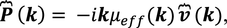 (45)
(45)with a upper hat designating Fourier’s transforms, \({\varvec{v}}\) the velocity field and \({\varvec{k}}\) the wavenumber whereas the viscosity \({\mu _{{\text{eff}}}}({\varvec{k}})\) is expressed by the following \({\varvec{k}}\)-dependent continued fraction
$${\mu _{{\text{eff}}}}(k)=\frac{\mu }{{1+\frac{{{k^2}l_{1}^{2}}}{{1+\frac{{{k^2}l_{2}^{2}}}{{1+ \ldots }}}}}},$$(46)where \(\mu\) is the viscosity of the bulk fluid in absence of nanostructures and \({l_n}\;(n=1,2, \ldots )\) are correlation lengths defined by \({l_n}^{2}=\beta _{n}^{2}/{\gamma _n}{\gamma _{n+1}}\) (e.g. Jou et al. 2010).

-
4.
In the applications considered above, there is only one reference length so that it is natural to select a one-dimensional wave number \(k\) as given by \(k=~2\pi /R\) and \(k=2\pi /H\) for cylindrical and parallepedic pores, respectively. Moreover, introducing a reference length \(l\), identified as the mean free path of the fluid particles through \(l_{n}^{2}={l^2}{n^2}/(4{n^2} - 1)\) (a well-known kinetic relation) and letting \(n \to \infty\), one obtains the final expression of the effective viscosity in terms of \(Kn\), namely
$${\mu _{{\text{eff}}}}=\frac{{3\mu }}{{4{\pi ^2}K{n^2}}}\left( {\frac{{2\pi ~Kn}}{{{\text{Arctan}}\left( {2\pi ~Kn} \right)}} - 1} \right).$$(47)
Rights and permissions
About this article

Cite this article
Machrafi, H., Lebon, G. Fluid flow through porous and nanoporous media within the prisme of extended thermodynamics: emphasis on the notion of permeability. Microfluid Nanofluid 22, 65 (2018). https://doi.org/10.1007/s10404-018-2086-9
Received:
Accepted:
Published:
DOI: https://doi.org/10.1007/s10404-018-2086-9