Korean East Coast wave predictions by means of ensemble Kalman filter data assimilation

Abstract

To respond to the need for preventing offshore and coastal accidents, damage and flooding, a state-of-the-art coastal wave forecast system for the East Coast of Korea waters is being developed. Given that the quality of the input wind has been identified as the main factor influencing the quality of the wave results, the effectiveness of adjusting the wind fields by means of data assimilation using the ensemble Kalman filter technique has been explored. In this article the model setup, the data assimilation parameters and the validation of the predictions during stormy periods is described. The validation shows that the model is able to provide predictions of coastal waves fulfilling available benchmarks; especially, the data assimilation analysis and forecast predictions are judged to be of high quality.

1 Introduction

The East Coast of Korea is prone to high wave action and an accurate wave forecast system is paramount for the prevention of offshore and coastal accidents, damage and flooding. To respond to this need, a state-of-the-art coastal wave forecast system for the East Coast of Korea waters is being developed. The first stage of this model development, namely the validation of the model in hindcast mode and the inclusion of data assimilation, is described in this article. Given the relevance of the depth effects on the coastal waves, the state-of-the-art shallow water wave model SWAN (Booij et al. 1999) has been chosen for the wave modelling. The left panel of Fig. 1 shows the bathymetry of the region covered by the wave model. The emphasis of the study is on the East Coast of Korea, the region covered by the observation locations (wind, waves) given on the right panel of Fig. 1. This stretch of coast has been subjected to a number of sea-related accidents with associated damages in the order of hundreds of billions of dollars and tens of life losses.

Fig. 1

Left: Arial view of the Eastern coast of Korea with an overlay of the bathymetry of the East Sea of Korea. The scale in metres of the bathymetry is given in the left. Right: Location of the observation sites

In the next section the general characteristics of the winds and waves affecting the East Coast of Korea are described along with a description of the available data. In Section 3, the developed wave model is described and, in Section 4, the applied data assimilation technique and its settings are described. A 32-day-long period—from 17 November 2015 until 16 December 2015—has been considered in the evaluation of the model hindcast, analysis and forecast. This period provides a variety of storm conditions allowing a proper assessment of the wave modelling and data assimilation, which is given in Section 5. The article ends with conclusions in Section 6.

2 Data and system understanding

2.1 General characteristics

In order to describe the mean wave climate in the region in more detail wind and wave reanalysis data from the European ReAnalysis interim (ERA-interim, Dee et al. 2011) dataset of the European Centre for Medium-range Weather Forecasts (ECMWF) has been used. The strength of the ERA-interim dataset is that it combines one of the leading numerical weather prediction models (the ECMWF model) with an advanced data assimilation system (Dee et al. 2011). The ERA-interim wave data are, therefore, known for its high quality, which is reflected in the high correlation between ERA-interim wave data and observations. However, due to its coarse resolution of about 80 km × 80 km the dataset is known to underestimate extreme wave events and of not being capable of fully solving tropical cyclones. Although, the data assimilation leads to (even for small systems) some tropical cyclone information being present in the ERA-interim data, the data are not suitable for analyses of tropical cyclones. The ERA-interim data from 1979 to 2016 is used next to provide a description of the wind and wave climate in the region, keeping the mentioned caveats due to resolution in mind.

The characteristics of the surface winds over the East Sea of Korea are illustrated by the annual rose of the 10 m height wind speed (U₁₀) and direction (U_dir) for a location offshore the Northeast coast of Korea (130.5° E, 37.5° N), see Fig. 2. These surface winds are generally mild or moderate and variable in summer and can be very strong in the winter, caused by low pressure systems in the East Asia winter monsoon. Typhoons occur from July through October, reaching their peak frequency in September. However, they generally move northward in the East Sea of Korea, not leading to extreme wave conditions along the East coast of Korea. Due to the regional monsoon variations, winds are predominantly from the Northwest to Northeast in the winter and more predominant from the northeast in the summer. Due to extra-tropical storms, there is a strong and predominant Western-Northwestern wind from November to February. Along the Northeastern coast of Korea the most frequent, extreme and longer waves come for the Northeast.

Fig. 2

Annual rose of ERA-interim wind speed data from 1979 to 2016 at 130.5° E and 37.5°N. The values plotted inside the circle on the centre of the rose represent the percentage of values that are below the lowest considered class of the variable being presented (e.g., below 1.5 m/s), the arrow length of each of the colours in the rose is the percentage of occurrence of conditions within a certain bin, the direction shown by each arrow/ray represents the direction from which winds (or waves) are coming from

Figure 3 shows the annual roses of significant wave height (H_s) and mean wave period¹ (T_{m − 1, 0}) and mean wave direction (MWD) for the same offshore location. As can be seen in Fig. 3, the most frequent, extreme and longer waves come for the Northeast. There are also extreme waves from the West-Northwest in line with the wind climate.

Fig. 3

Annual roses of ERA-interim significant wave height (top) and mean wave period (bottom) data from 1979 to 2016 at 130.5° E and 37.5° N

2.2 Observations

Along the Eastern coast of Korea wave and wind observations are available at the locations shown in Fig. 1. The coordinates of these locations, local depths and variables being observed are given in Table 1. Further details, such as the operator and the type of instrument, are also included. The observations are applied for both wave model validation as well as data assimilation.

Table 1 Coordinates and local depth of the observation locations, including the type of instruments installed and the responsible operator

2.3 Operational models

To develop a local wave model offshore wave boundary conditions and wind fields is needed. These have been sought for internally in KIOST and in KMA.

In order to benchmark the wave model results and force the offshore boundaries of the model, data have been collected from the following high-quality local wave models:

• KOOS-WAM: A coarse (20 km × 20 km) WAM cycle 4.5 model covering the region shown in Fig. 4 and operated by the project Korea Operational Oceanographic System (KOOS) of KIOST (Park et al. 2015).

• KOOS-WW3: A coarse (20 km × 20 km) WW3 model covering the same region as the KOOS-WAM model and with a finer resolution (4 km × 4 km) WW3 model covering the South Korean waters nested on it, see Fig. 4 (left panel). These nested WW3 models are also operated by the project KOOS of KIOST. The applied version of WW3 is 4.18 with ST3 physics (http://polar.ncep.noaa.gov/waves/wavewatch/manual.v4.18.pdf).

• KMA-CWW3: A coastal (1 km × 1 km) WW3 model (CWW3), which is nested in a regional (8 km × 8 km) WW3 model and which in turn is nested in a global (50 km × 50 km) WW3 model. The domains of the models, which are operated by the KMA, (http://web.kma.go.kr/eng/biz/forecast_02.jsp) are outlined in Fig. 4 (right panel).

Fig. 4

Left panel: Region covered by the coarse KOOS-WAM and KOOS-WW3 models, with the region covered by the nester finer resolution WW3 model outlined in green. The scale of the shown bathymetry is given in metres in the right. Right panel: Region covered by the coastal WW3 (CWW3) models operated by KMA. Results from the model with the domain outlined in green have been made available for this project

In order to force the wave model and to assess the wave model results, wind fields from the following local numeric weather prediction (NWP) models have been collected:

• KIOST-WRF: KIOST operates a Weather Research and Forecasting (WRF, http://www.wrf-model.org) model with 3D-VAR data (synop, sounding, buoy, scatterometer) assimilation (Heo and Ha 2016). The model domains are outlined in Fig. 5 (left panel). There is a wide domain with a 20 km × 20 km resolution with a smaller domain with a resolution of also 20 km × 20 km nested on it (there is still smaller domain with a finer resolution of 4 km × 4 km, but it does not cover the whole East Sea of Korea). The model gets initial conditions from the Global Forecast System (GFS) of the American National Centers for Environmental Prediction (NCEP). Hourly 10-m wind fields are available from the WRF model.

• KMA-UM: KMA operates a regional Unified Model (UM, https://en.wikipedia.org/wiki/Unified_Model) with four-dimensional variational data assimilation (4D-VAR), see http://web.kma.go.kr/eng/biz/forecast_02.jsp. Three-hourly 10 m wind fields with a spatial resolution of 12 km × 12 km are available from a regional UM model (referred to as Regional Data Assimilation and Prediction System, RDAPS). There is also a local UM model (referred to as Local Data Assimilation and Prediction System, LDAPS) with a spatial resolution of 1.5 km × 1.5 km and not covering the wave model domain and from which winds were not available for the considered period. Data from the fine resolution UM model is therefore not considered in this study. The domain covered by these models and given in Fig. 5.

Fig. 5

Left panel: Outline of the domains of the KIOST-WRF atmospheric model, for both domains the model resolution is 20 km × 20 km. Right panel: Outline of the domains of the KMA-UM atmospheric models, in the RDAPS domain the model resolution is 12 km × 12 km and in the LDAPS domain 1.5 km × 1.5 km

3 Wave model

3.1 Introduction

In order to obtain the best compromise between computational accuracy and efficiency, two nested models were employed, namely the

• Overall model—a coarse resolution model covering the East Sea of Korea (1500 km by 780 km) and the

• Coastal model—a finer resolution model covering the Northeastern coastal strip of South Korea (380 km by 100 km), extending from the coast into deep waters

Accordingly, the wave modelling is carried out in two stages with corresponding model domains which are outlined in Fig. 6. In these domains computational rectangular grids were defined in spherical coordinates (longitude, latitude) using the WGS84 geodetic datum.

Fig. 6

Left panel: Coverage and approximate dimensions of the overall (light blue) and coastal (white) model grids. Right panel: bathymetry of the coastal model

3.2 Overall model

A number of factors were taken into consideration in the definition of the overall model grid and domain. Recognising the primary importance of the waves generated in the East Sea of Korea to the Northeastern coast of Korea (cf. Section 2.1) the model was set to cover the whole East Sea of Korea. In order to also account for the relatively frequent waves entering the East Sea of Korea from the South, the model covers the Strait of Korea and extends into the East China Sea, where wave boundary conditions are imposed. The resolution of the overall model is of about 5 km × 5 km (about 45,000 active grid points). The model bathymetry, which is shown in Fig. 1, was derived from the American etopo5 database (http://www.ngdc.noaa.gov/mgg/global/etopo5.HTML) and the bathymetry of the coastal model in the region covered by it.

3.3 Coastal model

The purpose of the coastal model was to allow the modelling of depth effects with more resolution and therefore accuracy. The resolution of the coastal model is of about 300 m × 300 m (about 250,000 active grid points). The model extends from the coast into deep waters, covering the nearshore MB and WJ observation locations. The model bathymetry, which is shown in Fig. 6, was derived using the KorBathy30s bathymetry database (Seo 2008) and detailed survey data from KHOA with a resolution of about 150 × 150 m. Sensitivity tests have been carried out considering a grid with a resolution of about 150 m × 150 m, but the extra computational effort did not pay off in terms of accuracy of the results at the coastal buoy locations. Tests have also been carried out to check whether the increase in resolution from the overall model to the coastal model has been correctly modelled in the nesting, which seemed to be the case.

3.4 Directional and spectral grids

Each SWAN wave model requires the specification of three grid types:

• 1. a computational grid which defines the geographical location in 2D-space of the grid points and which have been described above;

• 2. a directional grid which defines the directional range (usually 360°) and resolution;

• 3. a spectral grid which defines the range and resolution of the grid in frequency space.

In both the overall and coastal models the same directional and spectral grids were defined. For directional space, the full circle is considered, divided in 48 sectors of 7.5° each. For the frequency domain frequencies were set to range from 0.03 to 1.5 Hz (0.67–33.33 s) logarithmically divided in 41 bins. These grid resolutions and ranges were chosen after a number of sensitivity tests (not shown). The high frequency range (1.5 Hz) is necessary for the accuracy of short-fetched growing seas.

3.5 Offshore boundary conditions

When the models will be operational, the wave parameters from the KOOS-WAM model will be available as spectral boundary conditions for the overall model. Figure 7 shows the locations of the KOOS-WAM data that are to be imposed in the southern boundaries of the overall model. These wave conditions are given parametrically in terms of significant wave height, peak wave period and mean wave direction. For each set of conditions, a JONSWAP spectrum (Hasselmann et al. 1973) is assumed in SWAN with a peak enhancement parameter of 3.3 and a directional spreading of about 31°. The conditions are set to vary linearly between two input locations along the model boundary. The conditions are kept constant between the coast line and the closest input location along the model boundary.

Fig. 7

Boundary locations of the overall model where wave boundary conditions are prescribed

3.6 Wind fields

When the models will be operational the KIOST-WRF winds will be available and used to force the coastal and overall models. It is, therefore, of importance to validate the models forced with the WRF winds. However, given that the coastal and overall model results will also be compared with KMA-WW3 model results it is also of interest to validate the results of the models forced with the KMA’s UM wind fields. Time and space varying wind fields from the KIOST-WRF model, with a spatial resolution of 20 km × 20 km and a temporal resolution of 1 h, are used to force the wave models. Furthermore, RDAPS time and space varying wind fields from the KMA-UM model, with a spatial resolution of 12 km × 12 km and a temporal resolution of 6 h, are used to force the wave models The wind fields resulting from the data assimilation, which have a spatial and temporal resolution equal to that of the first guess KIOST-WRF winds, will also be used to force the overall and coastal models.

3.7 Overall model settings

The SWAN wave modelling is carried out in non-stationary, 3rd generation mode for wind input, quadruplet interactions and whitecapping (wave steepness induced wave breaking). The default options of the applied SWAN version 40.85 are applied to all numerical and physics settings except for:

• Wind growth and whitecapping: Komen et al. (1984) with the settings recommended by Rogers et al. (2003) for wind growth and whitecapping is applied.

• Bottom friction: The JONSWAP formulation (Hasselmann et al. 1973) is applied with a friction coefficient of 0.038 m² s⁻³ as recommended by Zijlema et al. (2012).

• Numeric scheme: A first-order backward space, backward time (BSBT) scheme is applied.

• Integration time step: A fixed time step of 20 min is applied.

• Accuracy: The iterative solver is set to stop when the changes in the solution are of less than 1% in H_s and T_{m0, 1} at 99% of the grid points relatively to the previous iterations, with a maximum of 99 iterations per timestep.

The hydrodynamics of the East Sea is not taken into account, which means that currents are not incorporated and a uniform water level of 0 m MSL is considered in all computations.

4 Data assimilation

4.1 Introduction

The goal of data assimilation is to use (incorporate) observed data to improve the accuracy of model results. Data assimilation techniques range from those solely adjusting the model results directly to techniques deriving adjustments in the model input (such as forcing wind and spectral boundary conditions) and parameters so that the model results come closer to the observations. In this study, the goal is to reduce the differences between the Korean East Waters wave model results and the wave observations by adjusting the forcing wind fields. The state-of-the-art Ensemble Kalman Filter (EnKF) data assimilation technique has been chosen for this, since it has been successfully demonstrated in a SWAN model for the North Sea (Caires et al. 2018) and in a twin experiment using a coarse SWAN model of the Korean East Waters (Caires and Kim 2016). The details of the EnKF data assimilation are given in the next section. The EnKF computations are carried out using the Open Data Assimilation (OpenDA) toolbox (http://www.openda.org) to which the SWAN model is connected through a black-box wrapper. The settings of the applied EnKF data assimilation are given in Section 4.3.

4.2 Methodology

In an EnKF the model, uncertainty is computed from an ensemble of model predictions in a procedure very similar to Monte Carlo methods (Evensen 2003). The analysis or measurement-step of the EnKF uses a perturbation of the observations and a separate analysis for each of the ensemble members to obtain a consistent ensemble of model states that incorporate the observations if required one can obtain the mean and covariance of the model state after the analysis. More precisely, starting from an initial ensemble of model states ${\xi}_i^a\left({t}_0\right)$ the model M is used to compute a forecast for each ensemble member:

$$ {\xi}_i^f\left({t}_{k+1}\right)=M{\xi}_i^a\left({t}_k\right)+{w}_i\left({t}_k\right) $$

(1)

where w_i(t_k) denotes the system noise used to model uncertainties in the model. From this, one can compute the sample mean as

$$ {x}^f\left({t}_k\right)=\frac{1}{n}\sum \limits_{i=1}^n{\xi}_i^f\left({t}_k\right) $$

(2)

and covariance

$$ {\mathbf{P}}^f\left({t}_k\right)=\frac{1}{\left(n-1\right)}\sum \limits_{i=1}^n\left({\xi}_i^f\left({t}_k\right)-{x}^f\left({t}_k\right)\right){\left({\xi}_i^f\left({t}_k\right)-{x}^f\left({t}_k\right)\right)}^{\prime } $$

(3)

The Kalman gain is expressed as

$$ \mathbf{K}\left({t}_k\right)={\mathbf{P}}^f\left({t}_k\right){\mathbf{H}}^{\prime }{\left(\mathbf{H}{\mathbf{P}}^f\left({t}_k\right){\mathbf{H}}^{\prime }+\mathbf{R}\right)}^{-1} $$

(4)

where H denotes the observation operator that maps the model state to values that match the observations. R is the error covariance of the observations at time t_k.

The analysis or measurement-step of the EnKF uses a perturbation of the observations v_i(t_k) and a separate analysis for each of the ensemble members to obtain a consistent ensemble of states that incorporate the observations y(t_k),

$$ {\xi}_i^a\left({t}_k\right)={\xi}_i^f\left({t}_k\right)+\mathbf{K}\left({t}_k\right)\left(y\left({t}_k\right)-H{\xi}_i^f\left({t}_k\right)-{v}_i\left({t}_k\right)\right) $$

(5)

If required one can obtain the mean and covariance of the model state after the analysis, that can be computed from

$$ {x}^a\left({t}_k\right)=\frac{1}{n}\sum \limits_{i=1}^n{\xi}_i^a\left({t}_k\right) $$

(6)

and

$$ {\mathbf{P}}^a\left({t}_k\right)=\frac{1}{\left(n-1\right)}\sum \limits_{i=1}^n\left({\xi}_i^a\left({t}_k\right)-{x}^a\left({t}_k\right)\right){\left({\xi}_i^a\left({t}_k\right)-{x}^a\left({t}_k\right)\right)}^{\prime } $$

(7)

The OpenDA implementation for SWAN uses the full wave spectra at all grid-cells as the state of the model. Two likely sources of uncertainty in a spectral wave model are the uncertainty in the wind forcing and uncertainty for the wave parameters that are specified at the open-boundary. Both sources can be considered in the OpenDA implementation of EnKF for SWAN (see e.g. Serpoushan et al. 2013).

4.3 Settings

The results of the EnKF data assimilation in SWAN are sensitive to a number of parameters, such as 1) uncertainty in the specification of the forcing winds and spectral boundary conditions (the so-called control variables), 2) which data are assimilated and their uncertainty and 3) the number of EnKF ensemble members:

• 1) In this study, we only considered uncertainty for the wind forcing. The uncertainty in the spectral boundary conditions is not considered to be as crucial for the quality of the results and is, therefore, not considered in these experiments. The used (first-guess) wind fields are the WRF fields. For the uncertainty in the wind forcing, the two wind components are treated independently. For each component, the errors are assumed to be spatially and temporally correlated with an exponential decay with distance and time-difference. Namely, the covariance of the errors is expressed as

$$ \mathit{\operatorname{cov}}\left({x}_1,{x}_2\right)={\sigma}_{x1}{\sigma}_{x2}\exp \left(-\frac{\left|l-{l}_0\right|}{L}\right)\exp \left(-\frac{\left|t-{t}_0\right|}{T}\right) $$

(8)

with standard deviations of the errors, σ_x1 and σ_x2, being set to 1 m/s and the temporal and spatial correlation lengths, T and L, set to respectively 12 h and 500 km. These values have been chosen after sensitivity computations (not shown here).

• 2) Observations of H_s have been assimilated every hour at the further offshore DH and E01 locations (cf. Fig. 1). The errors in the observations are assumed uncorrelated and Gaussian with a standard deviation of 0.2 m (in accordance with buoy measurement accuracy).

• 3) Experimental runs were carried out with 10, 30 and 100 ensemble members. The number of ensemble members did not affect the results much but the observation minus model statistics of the run with 30 ensembles was slightly better.

To reduce the EnKF computational effort the overall model computational grid has been coarsened nine times in each direction from a resolution of 0.05° × 0.05° to a resolution of 0.45° × 0.45°, see Fig. 8. Furthermore, although SWAN can read wind fields in curvilinear grids that is not the case for OpenDA, which only supports rectangular grids for the wind. The WRF input winds had therefore to be mapped into a rectangular grid for the EnKF experiments. The used rectangular grid had a resolution close to that of the original WRF fields, see Fig. 8. The resulting analysis wind fields have then been used to force the full (not coarsened) overall model and nested coastal model.

Fig. 8

Left panel: Grid of the overall model (blue) and grid of the model used in the EnKF runs (red). Rigth panel: Grid of the KIOST-WRF winds used in the hindcast (blue) and grid of the winds used in the EnKF runs (red)

5 Analysis of the results

5.1 Hindcast and analysis

Three sets of forcing winds are considered in the SWAN computations and validation:

• KIOST-WRF (cf. Section 2.3);

• KMA-UM (cf. Section 2.3) and

• EnKF: The winds resulting from the EnKF data assimilation in which the KIOST-WRF were used as input.

Figures 9, 10, 11, 12 show the time series comparisons between the U₁₀, U_dir observations and the KIOST-WRF and KMA-UM hindcasts and EnKF analysis at DH, UL, E01 and E02.

Fig. 9

Time series of the DH wind observations and KIOST-WRF, KMA-UM and EnKF winds

Fig. 10

Time series of the UL wind observations and KIOST-WRF, KMA-UM and EnKF winds

Fig. 11

Time series of the E01 wind observations and KIOST-WRF, KMA-UM and EnKF winds

Fig. 12

Time series of the E02 wind observations and KIOST-WRF, KMA-UM and EnKF winds

Six sets of wave model results are considered:

• SWAN: The (default) SWAN hindcast with the KIOST-WRF wind forcing;

• SWAN-UM: The SWAN hindcast with the KMA-UM wind forcing;

• SWAN-EnKF: The SWAN analysis with the EnKf winds

• KMA-CWW3; KOOS-WW3 and KOOS-WAM (cf. Section 2.3).

Figures 13, 14, 15, 16, 17, 18 show the time series comparisons between the H_s, T_p and MWD observations and the model results at MB, WJ, DH, UL, E01 and E02.

Fig. 13

Time series of the MB wave observations and wave model results

Fig. 14

Time series of the WJ wave observations and wave model results

Fig. 15

Time series of the DH wave observations and wave model results

Fig. 16

Time series of the UL wave observations and wave model results

Fig. 17

Time series of the E01 wave observations and wave model results

Fig. 18

Time series of the E02 wave observations and wave model results

During this period three storm periods (delineated with vertical dashed red lines in Figs. 9, 10, 11, 12, 13, 14, 15, 16, 17, 18) have been examined in more detail:

• Storm 1—from 25 November 13:00 until 28 November 23:00 KST—The period started with winds from Northeast over the whole East Sea of Korea followed by a strong cyclone with winds still from Northeast on the north-western side of the East Sea of Korea and rotating to North in the Tongjoson Man bay (offshore North Korea) and rotating further to Northwest in the southern part of the East Sea of Korea. The centre of the cyclone moves then further in the Northeast direction and the winds become predominantly from the Northwest along the coast of Korea and the Southern part of the East Sea of Korea. Figure 19 shows a snapshot of the KIOST-WRF winds and overall and coastal model waves during this period. During this period the observed significant wave height is above 4 m nearshore and above 6 m offshore, the peak wave period is above 12 s and waves propagate from the Northeast nearshore and mostly Northwest offshore, although at UL (Fig. 16) and E01 (Fig. 17) waves are mostly towards the coast. Wind speeds peak at about 20 m/s at E01 offshore and blow from Northwest (Fig. 11).

  Fig. 19

  

  Snapshot of the overall and coastal model significant wave height and direction (left and middle panels) and KIOST-WRF wind fields (right panel) during Storm 1

• Storm 2—from 3 December 13:00 until 6 December 23:00 KST—the period started with winds from the West over the southern part of the East Sea of Korea which increased and got a more north-westerly direction, leading to high waves along the coast of Japan. Figure 20 shows a snapshot of the KIOST-WRF winds and overall and coastal model waves during this period. The wave conditions observed nearshore are very mild, with the significant wave height well below the 2 m and the peak wave period below 10 s, offshore the significant wave height can be as high as 5 m in E01 (Fig. 17). There are no wind observations at DH during this period (Fig. 9) and at E02 during the start of the period (Fig. 12). At E01 (Fig. 11) and UL (Fig. 10) the observed winds are from the West-Northwest and at most 17 m/s.

  Fig. 20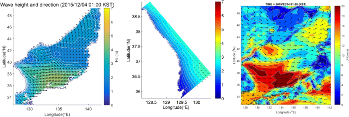

  

  Snapshot of the wave height and direction (left and middle panels) and wind fields (right panel) during Storm 2

• Storm 3—from 11 December 00:00 until 15 December 12:00 KST—the period started with winds from Northeast over the whole East Sea of Korea which increased and got a more northern direction. Figure 21 shows a snapshot of the KIOST-WRF winds and overall and coastal model waves during this period. The observed waves are from the Northeast, the peak significant wave height is about 5 m nearshore and above 6 m offshore; the peak wave period is about 10 s. Offshore the observed winds are also from the northeast ranging between 15 and 20 m/s.

  Fig. 21

  

  Snapshot of the wave height and direction (left and middle panels) and wind fields (right panel) during Storm 3

Root-mean-square errors based on the whole 2015 period have been determined for both the wind velocity (speed and direction) and the resulting wave parameters, making a distinction between the forcing by WRF, EnKF and UM model winds. For wind speed and direction these errors are given in Table 2 for four locations. For six locations, the root-mean-square errors for significant wave height, peak wave period and mean wave direction are given in Fig. 22. All six models descried at the start of this section are considered. In addition, and in order to assess the effects of the data assimilation in more detail, Figs. 23, 24, 25, 26, 27, 28 show scatter comparisons between the significant wave height observations and the SWAN and the SWAN-EnKF results.

Table 2 Root-mean-square-errors in metres for the wind speed and wind direction (RMSE) of the atmospheric models KIOST-WRF and KMA-UM and determined by EnKF wind speeds and directions

Fig. 22

Root-mean-square-error (RMSE) of the wave model results for 2015

Fig. 23

Density scatter comparison between the significant wave height observations and the corresponding SWAN (left panel) an SWAN-EnKF data at MB. The symmetric slope (red line) and the correlation between the data are printed in red in the figure

Fig. 24

Same as Fig. 23 but at WJ

Fig. 25

Same as Fig. 23 but at DH

Fig. 26

Same as Fig. 23 but at UL

Fig. 27

Same as Fig. 23 but at E01

Fig. 28

Same as Fig. 23 but at E02

The following conclusions are taken from the analyses of the comparisons:

• At the coastal locations MB and WJ (Fig. 13 and Fig. 14) all models seem to follow the observation relatively well. All models overestimate the observed and relatively low significant wave height in Storm 2, except for the KMA-CWW3 model. Especially at MB, all models provide predictions very close to the observations during Storm 3. From the 17th of December the MWD data of KIOST-WW3 is erroneously taking a fixed value of 180°N. No data from these locations have been assimilated but still the SWAN-EnKF results compare better with the H_s and T_p observations than those of SWAN. Especially during Storm 2 the SWAN-EnKF H_s and T_p data follow closer the observations. Figure 29 shows a comparison between the observed, SWAN and SWAN-EnKF frequency spectra during the peak of Storm 1 at MB (left panel) and during the peak of Storm 2 at WJ (right panel). As can be seen in the figure, the SWAN-EnKF spectra are closer to the observations. More specific, in the Storm 1 example, all spectra are close. In the Storm 2 example, although the assimilated SWAN-EnKF spectrum overestimates the observed frequency spectrum, a significant improvement is obtained from data assimilation.

• At nearshore DH location and offshore UL location (Fig. 15 and Fig. 16) the comparisons between the model significant wave height and peak wave period predictions and the observations are similar to those with the MB and WJ locations. Waves at these deep water locations are not directly affected by the bathymetry and the performance of the models in terms of wave direction is comparable. The H_s observations from DH have been assimilated and the H_s RMSE of SWAN-EnKF is consequently much lower than that of the other models (cf. Fig. 22).

• At the further offshore E01 (Fig. 17) location all models seem to follow the significant wave height and mean wave direction observations relatively well. Except for the KMA-CWW3 model and the SWAN-EnKf results, all models underestimate the wave height in Storm 2, which at this location correspond to high significant wave heights, as high as those during Storm 3.

• There are no wave observations available from E02 (Fig. 18) during the period between the 15th of November and the 4th of December. During the period with observations the comparisons between the model predictions and the observations are similar to those at UL. Although the E02 data has not been assimilated, the RMSE of the SWAN-EnKF results is about half of that of the SWAN results (cf. Fig. 22).

• The WRF, EnKF and UM wind predictions follow the observations reasonably well (Figs. 9, 10, 11, 12) and show comparable error statistics with the RMSE of the WRF winds being slightly lower (Table 2). At location E02 there are no observations during the Storm 1 (Fig. 12). At the other locations the models tend to overestimate the wind speed, especially during the second half of the Storm 1. At location DH, there are no observations during the Storm 2 (Fig. 9) and at all other locations the WRF and UM models overestimate the observed wind speeds. The EnKF data assimilation is successful in reducing the overestimation of the original WRF winds. Both the WRF and the UM predictions compare well with the observed wind speed peak during the Storm 3.

Fig. 29

Example of the effect of the data assimilation on the frequency spectrum. Left panel: Data from MB during storm 1 (6:00 27 November 2015). Right panel: Data from WJ during storm 2 (3:00 4 December 2015)

From these comparisons, it can be concluded that the original SWAN model (so without resorting to data assimilation) already provided results with at least the same quality as that of the existing models for the region. The errors in the wave predictions seem to be mostly due to errors in the wind predictions, with the EnKF data assimilation leading to results closer to the observations. In fact the EnKF leads for the whole period to reductions in the RMSE of H_s and T_p of up to 38 and 7%, respectively, in the locations where the data were assimilated (DH and E01, cf. Fig. 22). At the other locations (MB, WJ, UL and E02), the reductions were of up to 49% and 19% in the H_s and T_p′ RMSEs, respectively (cf. Fig. 22). The differences in the RMSE of the mean wave direction (MWD) are not statistically significant. For the period of the second storm, the reductions in the RMSE are the largest (not shown) and of up to 66% and 42% in the H_s and T_p′ RMSE in the locations where the data were assimilated (DH and E01) and 75% and 36% in the H_s and T_p′ RMSE in the locations where the data were not assimilated (MB, WJ, UL and E02).

From the analysis of the errors in the KMA-CWW3 model, results and UM winds is unclear whether the UM winds are indeed those that have been used to force the KMA-CWW3 model. Specifically, the CWW3 results do not overestimate the wave conditions during the second storm period whereas the UM winds overestimate the observations and lead to wave height overestimates in the other models.

5.2 Forecasts

In order to assess until when the model forecast are affected by the data assimilation, 48-h forecasts have been carried out at each time step from 19 November 2015 until 15 December 2015 using the wave field and wind field from the data assimilation at forecast timestep 0 h and the original WRF wind fields in the consecutive hours. Given the computational effort involved only the overall model has been run in these forecasts. The RMSE variation with the forecast hour is shown in Fig. 30 for the measuring locations covered only by the overall model, namely DH, UL, E01 and E02. The figure shows also the RMSE of the 0 h hindcast and the 0 h analysis, the model results referred to as SWAN and SWAN-EnKF, respectively, in the previous section (cf. Fig. 22). The figure shows that the positive effects of the data assimilation last for about 12 h for the significant wave height and about 24 h for the peak wave period. The significant wave height forecast RMSE for forecast times above 12 h generally slightly overshoots the hindcast error. This is due to the iterative procedure of SWAN, which differences in analysis (+0 h) and forecast winds (+1 h) lead to (convergence) differences which still remain when the waves are no longer affected by these initial (0 h and + 1 h) fields. The same applies for the peak wave period forecast RMSE, which at UL the analysis RMSE was higher than the hindcast RMSE, but the forecast RMSE is in the first 20 forecast hours below both of them (cf. right panel in the second row of Fig. 30).

Fig. 30

Root-mean-square-error (RMSE) of the wave model forecast. Left column: Significant wave height. Right column: Peak wave period. The red line indicates the RMSE of the 0 h hindcast, the green line indicates the RMSE of the 0 h analysis and the blue line gives the RMSE of the +1 h to +48 h forecast

6 Conclusions

A SWAN wave model with EnKF data assimilation is being developed to respond to the need of wave forecasts for the East Coast of Korea. The validation of the model hindcasts during the considered storm period shows that the model results are at least as accurate as those of other high-quality local models. The main contributor to the model errors appears to be the errors in the forcing wind fields. The EnKF assimilation of offshore significant wave height observations with the winds as control variable leads to reductions in the root-mean-square-error at locations other than those where the data were assimilated of about 50% and in the peak wave period of about 20%. The positive effects of the data assimilation decrease with forecast time but remain positive at least in the first 12 forecast hours. The further development of the system will involve a sensitivity study to which other wave parameters should be assimilated and from which observation locations.

References

Booij N, Ris RC, Holthuijsen LH (1999) A third generation wave model for coastal regions. Part 1. Model description and validation. J Geophys Res 104(C4):76497666
Caires S, Kim J (2016) On the development of an operational wave forecast system for the Korean East coast: description, assessment and further developments. Deltares report 1230243-000-HYE-0005: p. 84
Caires S, Marseille GJ, Verlaan M, Stoffelen A (2018) North Sea wave analysis using data assimilation and mesoscale model forcing winds. J Waterw Port Coast Ocean Eng 144 (4), https://doi.org/10.1061/(ASCE)WW.1943-5460.0000439
Dee DP et al (2011) The ERA-interim reanalysis: configuration and performance of the data assimilation system. Q J R Meteorol Soc 137(656):553–597. https://doi.org/10.1002/gj.828
Evensen G (2003) The ensemble Kalman filter: theoretical formulation and practical implementation. Ocean Dyn 53:343–367
Hasselmann K, Barnett TP, Bouws E, Carlson H, Cartwright DE, Enke K, Ewing JA, Gienapp H, Hasselmann DE, Kruseman P, Meerburg A, Mller P, Olbers DJ, Richter K, Sell W, Walden H (1973) Measurements of wind-wave growth and swell decay during the Joint North Sea Wave Project (JONSWAP). Deutsche hydrographische Zeitschrift, A(8), Nr. 12, p.95
Heo K-Y, Ha T (2016) Producing the Hindcast of Wind and Waves Using a High-Resolution Atmospheric Reanalysis around Korea. Journal of Coastal Research: Special Issue 75 - Proceedings of the 14th International Coastal Symposium, 1107–1111, Sydney 6–11 March 2016
Komen GJ, Hasselmann S, Hasselmann K (1984) On the existence of a fully developed windsea spectrum. J Phys Oceanogr 14:1271–1285
Park K-S, Heo K-Y, Jun K, Il Kwon J, Kim J, Choi J-Y, Cho K-H, Choi B-J, Seo S-N, Kim YH, Kim S-D, Yang C-S, Lee J-C, Kim S-I, Kim S, Choi J-W, Jeong S-H (2015) Development of the operational oceanographic system of Korea. J Ocean Sci 50(2):353–369. https://doi.org/10.1007/s12601-015-0033-1
Rogers WE, Hwang PA, Wang DW (2003) Investigation of wave growth and decay in the SWAN model: three regional-scale applications. J Phys Oceanogr 33:366–389
Seo S-N (2008) Digital 30 sec gridded bathymetric data of Korea marginal seas - KorBathy30s (in Korean). JKSCOE 20(1):110–120
Serpoushan N, Zeinoddini M, Golestani M (2013) An ensemble kalman filter data assimilation scheme for modeling the wave climate in Persian Gulf. Proceedings of OMAE 2013, June 9–14, 2013, Nantes, France
Zijlema M, van Vledder GP, Holthuijsen LH (2012) Bottom friction and wind drag for wave models. Coast Eng 65:19–26
Acknowledgments
We are thankful to ECMWF, KMA, KHOA and the KOOS project of KIOST for the having been able to access and use their data.
Funding
We are, furthermore, grateful to the Korean Government for funding. This research was part of a project entitled “Construction of Ocean Research Station and their Application Studies” which was funded by the Ministry of Oceans and Fisheries, South Korea.
Author information
Authors and Affiliations
Corresponding author
Additional information
Responsible Editor: Oyvind Breivik
This article is part of the Topical Collection on the 15th International Workshop on Wave Hindcasting and Forecasting in Liverpool, UK, September 10-15, 2017
Rights and permissions
About this article
Cite this article
Caires, S., Kim, J. & Groeneweg, J. Korean East Coast wave predictions by means of ensemble Kalman filter data assimilation. Ocean Dynamics 68, 1571–1592 (2018). https://doi.org/10.1007/s10236-018-1214-0
Received:
Accepted:
Published:
Issue Date:
DOI: https://doi.org/10.1007/s10236-018-1214-0