
Abstract
In this paper, we introduced some similarity measures for bipolar neutrosophic sets such as; Dice similarity measure, weighted Dice similarity measure, Hybrid vector similarity measure and weighted Hybrid vector similarity measure. Also we examine the propositions of the similarity measures. Furthermore, a multi-criteria decision-making method for bipolar neutrosophic set is developed based on these given similarity measures. Then, a practical example is shown to verify the feasibility of the new method. Finally, we compare the proposed method with the existing methods in order to demonstrate the practicality and effectiveness of the developed method in this paper.
1 Introduction
As a generalization of classical sets, fuzzy set [51] and intuitionistic fuzzy set [3], neutrosophic set was presented by Smarandache [32, 33] to capture the incomplete, indeterminate and inconsistent information. The neutrosophic set has three completely independent parts, which are truth-membership degree, indeterminacy-membership degree and falsity-membership degree; therefore, it is applied to many different areas, such as decision-making problems [1, 2, 4, 7–11, 19, 23, 31, 37–39, 42, 52]. In additionally, since the neutrosophic sets are hard to be applied in some real problems because of the truth-membership degree, indeterminacy-membership degree and falsity-membership degree lie in \({]}^-0,1^+{[}\), single-valued neutrosophic sets introduced by Wang et al. [40].
Recently, Lee [21, 22] proposed notation of bipolar fuzzy set and their operations based on fuzzy sets. A bipolar fuzzy set has two completely independent parts, which are positive membership degree \(T^+\rightarrow [0,1]\) and negative membership degree \(T^-\rightarrow [-1,0]\). Also the bipolar fuzzy models have been studied by many authors including theory and applications in [12, 17, 25, 34, 35, 50]. After the definition of Smarandache’s neutrosophic set, neutrosophic sets and neutrosophic logic have been applied in many real applications to handle uncertainty. The neutrosophic set uses one single value in \({]}^-0,1^+{[}\) to represent the truth-membership degree, indeterminacy-membership degree and falsity-membership degree of an element in the universe X. Then, Deli et al. [18] introduced the concept of bipolar neutrosophic sets, as an extension of neutrosophic sets. In the bipolar neutrosophic sets, the positive membership degree \(T^{+}(x),\,I^{+}(x),\,F^{+}(x)\) denotes the truth membership, indeterminate membership and false membership of an element \(x\in X\) corresponding to a bipolar neutrosophic set A and the negative membership degree \(T^{-}(x),\,I^{-}(x),\,F^{-}(x)\) denotes the truth membership, indeterminate membership and false membership of an element \(x\in X\) to some implicit counter-property corresponding to a bipolar neutrosophic set A.
Similarity measure is an important tool in constructing multi-criteria decision-making methods in many areas such as medical diagnosis, pattern recognition, clustering analysis, decision making and so on. Similarity measures under all sorts of fuzzy environments including single-valued neutrosophic environments have been studied by many researchers in [5, 6, 13, 14, 15, 20–24, 26–30, 43–49]. Also, Deli and Şubas’s [16] and Şahin et al. [36] presented some similarity measures on bipolar neutrosophic sets based on correlation coefficient similarity measure and Jaccard vector similarity measure of neutrosophic set and applied to a decision-making problem, respectively. This paper is constructed as follows. In Sect. 2, some basic definitions of neutrosophic sets and bipolar neutrosophic sets are introduced. In Sect. 3, we propose some similarity measures for bipolar neutrosophic sets such as; Dice similarity measure, weighted Dice similarity measure, Hybrid vector similarity measure and weighted Hybrid vector similarity measure and investigate their several properties. In Sect. 4, a multi-criteria decision-making method for bipolar neutrosophic set is developed based on these given similarity measures and a practical example is given. In Sect. 5, we compare the proposed method with the existing methods in order to demonstrate the practicality and effectiveness of the developed method in this paper. In Sect. 6, the conclusions are summarized.
2 Preliminary
In the section, we give some concepts related to neutrosophic sets and bipolar neutrosophic sets.
Definition 1
[32] Let E be a universe. A neutrosophic set A over E is defined by
where \(T_A(x)\), \(I_A(x)\) and \(F_A(x)\) are called truth-membership function, indeterminacy-membership function and falsity-membership function, respectively. They are, respectively, defined by
such that \(0^-\le T_A(x) + I_A(x) + F_A(x)\le 3^+\).
Definition 2
[40] Let E be a universe. A single-valued neutrosophic set (SVN-set) A over E is defined by
where \(T_A(x)\), \(I_A(x)\) and \(F_A(x)\) are called truth-membership function, indeterminacy-membership function and falsity-membership function, respectively. They are respectively defined by
such that \(0\le T_A(x) + I_A(x) + F_A(x)\le 3\).
Definition 3
[18] A bipolar neutrosophic set(BNS) A in X is defined as an object of the form
where
The positive membership degree \(T^{+}(x),\,I^{+}(x),\,F^{+}(x)\) denotes the truth membership, indeterminate membership and false membership of an element \(x\in X\) corresponding to a bipolar neutrosophic set A and the negative membership degree \(T^{-}(x),\,I^{-}(x),\,F^{-}(x)\) denotes the truth membership, indeterminate membership and false membership of an element \(x\in X\) to some implicit counter-property corresponding to a bipolar neutrosophic set A.
Definition 4
[18] Let \(A_{1}=\langle x,T_{1}^{+}(x),I_{1}^{+}(x),F_{1}^{+}(x), T_{1}^{-}(x),I_{1}^{-}(x),F_{1}^{-}(x)\rangle\) and \(A_{2}=\langle x,T_{2}^{+}(x),I_{2}^{+}(x),F_{2}^{+}(x), T_{2}^{-}(x),I_{2}^{-}(x),F_{2}^{-}(x)\rangle\) be two BNSs in a universe of discourse X. Then the following operations are defined as follows:
-
1.
\(A_{1}=A_{2}\) if and only if \(T_{1}^{+}(x)=T_{2}^{+}(x),I_{1}^{+} (x)=I_{2}^{+}(x),F_{1}^{+}(x)=F_{2}^{+}(x)\) and \(T_{1}^{-}(x)=T_{2}^{-}(x),I_{1}^{-}(x) =I_{2}^{-}(x),F_{1}^{-}(x)=F_{2}^{-}(x).\)
-
2.
\(\begin{aligned} A_{1}\cup A_{2}= &{} \{\langle x,max(T_{1}^{+}(x),T_{2}^{+}(x)), \frac{I_{1}^{+}(x)+I_{2}^{+}(x)}{2},min(F_{1}^{+}(x),F_{2}^{+}(x)), \\ &{} min(T_{1}^{-}(x),T_{2}^{-}(x)),\frac{I_{1}^{-}(x)+I_{2}^{-}(x)}{2},max(F_{1}^{-}(x),F_{2}^{-}(x))\rangle \} \end{aligned}\) \(\forall x\in X.\)
-
3.
\(\begin{aligned} A_{1}\cap A_{2}=&{} \{\langle x,min(T_{1}^{+}(x),T_{2}^{+}(x)),\frac{I_{1}^{+}(x)+I_{2}^{+}(x)}{2},max(F_{1}^{+}(x),F_{2}^{+}(x)), \\ &{}max(T_{1}^{-}(x),T_{2}^{-}(x)),\frac{I_{1}^{-}(x)+I_{2}^{-}(x)}{2},min(F_{1}^{-}(x),F_{2}^{-}(x))\rangle \} \end{aligned}\) \(\forall x\in X.\)
-
4.
\(A^c= \{\langle x, 1-T_{A}^{+}(x),1-I_{A}^{+}(x), 1-F_{A}^{+}(x), 1-T_{A}^{-}(x),1-I_{A}^{-}(x), 1-F_{A}^{-}(x)\rangle \}\)
-
5.
\(A_{1}\subseteq A_{2}\) if and only if \(T_{1}^{+}(x)\le T_{2}^{+}(x), I_{1}^{+}(x)\le I_{2}^{+}(x),F_{1}^{+}(x)\ge F_{2}^{+}(x)\) and \(T_{1}^{-}(x)\ge T_{2}^{-}(x),I_{1}^{-}(x)\ge I_{2}^{-}(x),F_{1}^{-}(x)\le F_{2}^{-}(x).\)
Definition 5
[45] Let \(A=\langle T_{A}(x_{i}),I_{A}(x_{i}),F_{A}(x_{i})\rangle\) and \(B=\langle T_{B}(x_{i}),I_{B}(x_{i}),F_{B}(x_{i})\rangle\) be two SVNSs in a universe of discourse \(X=(x_{1},x_{2},\ldots,x_{n}).\) Then Dice similarity measure between SVNSs A and B in the vector space is defined as follows:
It satisfies the following properties:
-
1.
\(0\le D(A,B)\le 1;\)
-
2.
\(D(A,B)=D(B,A);\)
-
3.
\(D(A,B)=1\) for \(A=B\) i.e.\(T_{A}(x_{i})=T_{B}(x_{i}), I_{A}(x_{i})=I_{B}(x_{i}),F_{A}(x_{i})=F_{B}(x_{i})(i=1,2\ldots ,n)\ \ \forall \ x_{i} (i=1,2,\ldots ,n)\in X.\)
Definition 6
[29] Let \(A=\langle T_{A}(x_{i}),I_{A}(x_{i}),F_{A}(x_{i})\rangle\) and \(B=\langle T_{B}(x_{i}),I_{B}(x_{i}),F_{B}(x_{i})\rangle\) be two SVN-sets in a universe of discourse \(X=(x_{1},x_{2},\ldots ,x_{n}).\) Then
It satisfies the following properties:
-
1.
\(0\le E(X,Y)\le 1;\)
-
2.
\(E(X,Y)=E(Y,X);\)
-
3.
\(E(X,Y)=1\) for \(X=Y\) i.e.,\(x_{i}=y_{i}(i=1,2\ldots ,n)\forall x_{i} \in X\ and\ y_{i}\in Y.\)
3 Similarity measures of bipolar neutrosophic sets
In this section, we introduce some similarity measures for bipolar neutrosophic sets including Dice similarity measure, weighted Dice similarity measure, Hybrid vector similarity measure and weighted Hybrid vector similarity measure by extending the studies in [29, 45].
Definition 7
Let \(A=\langle T_{A}^{+}(x_{i}),I_{A}^{+}(x_{i}),F_{A}^{+}(x_{i}),T_{A}^{-}(x_{i}), I_{A}^{-}(x_{i}),F_{A}^{-}(x_{i})\rangle\) and \(B=\langle T_{B}^{+}(x_{i}),I_{B}^{+}(x_{i}),F_{B}^{+}(x_{i}),T_{B}^{-}(x_{i}),I_{B}^{-}(x_{i}),F_{B}^{-}(x_{i})\rangle\) be two BNSs in the set \(X=\{x_{1},x_{2},\ldots ,x_{n}\}.\) Then, Dice similarity measure between BNS A and B, denoted D(A, B), is defined as;
Example 1
Suppose that \(A=\langle 0.5,0.2,0.6,-0.4,-0.3,-0.7\rangle\), \(B=\langle 0.7,0.1,0.3,-0.2,-0.2,-0.1\rangle\) be two BNSs in the set. Then,
Definition 8
Let \(A=\langle T_{A}^{+}(x_{i}),I_{A}^{+}(x_{i}),F_{A}^{+}(x_{i}),T_{A}^{-}(x_{i}), I_{A}^{-}(x_{i}),F_{A}^{-}(x_{i})\rangle\) and \(B=\langle T_{B}^{+}(x_{i}),I_{B}^{+}(x_{i}),F_{B}^{+}(x_{i}),T_{B}^{-}(x_{i}), I_{B}^{-}(x_{i}),F_{B}^{-}(x_{i})\rangle\) be two BNSs in the set \(X=\{x_{1},x_{2},\ldots ,x_{n}\}\) and \(w_{i}\in [0,1]\) be the weight of each element \(x_{i}\) for \(i=1,2,\ldots ,n\) such that \(\sum _{i=1}^{n}w_{i}=1\). Then, weighted Dice similarity measure between BNS A and B, denoted \(D_{w}(A,B)\), is defined as;
Example 2
Suppose that \(A=\langle 0.8,0.2,0.5,-0.2,-0.3,-0.4\rangle\), \(B=\langle 0.6,0.4,0.3,-0.1,-0.2,-0.3\rangle\) be two BNSs in the set and \(w=0.3\). Then,
Proposition 1
Let \(D_{w}(A,B)\) be a weighted Dice similarity measure between BNSs A and B. Then, we have
-
1.
\(0\le D_{w}(A,B)\le 1;\)
-
2.
\(D_{w}(A,B)=D_{w}(B,A);\)
-
3.
\(D_{w}(A,B)=1\) for \(A=B\) i.e.,\(T_{A}^{+}(x_{i})=T_{B}^{+}(x_{i}),I_{A}^{+}(x_{i})=I_{B}^{+}(x_{i}), F_{A}^{+}(x_{i})=F_{B}^{+}(x_{i}),T_{A}^{-}(x_{i})=T_{B}^{-}(x_{i}), I_{A}^{-}(x_{i})=I_{B}^{-}(x_{i}),F_{A}^{-}(x_{i})=F_{B}^{-}(x_{i})(i=1,2\ldots ,n)\ \ \forall \ x_{i} (i=1,2,\ldots ,n)\in X.\)
Proof
-
1.
It is clear from Definition 8.
-
2.
$$\begin{aligned} D_{w}(A,B)& =\sum _{i=1}^{n}w_{i}\\& \quad \, { \times \begin{array}{c} \left( \begin{array}{r} \frac{\begin{array}{l} [(T_{A}^{+}(x_{i})T_{B}^{+}(x_{i})+I_{A}^{+}(x_{i})I_{B}^{+}(x_{i})+F_{A}^{+}(x_{i})F_{B}^{+}(x_{i})){-}(T_{A}^{-}(x_{i})T_{B}^{-}(x_{i})+I_{A}^{-}(x_{i})I_{B}^{-}(x_{i})+F_{A}^{-}(x_{i})F_{B}^{-}(x_{i}))] \end{array}}{\begin{array}{l} [((T_{A}^{+})^{2}(x_{i})+(I_{A}^{+})^{2}(x_{i})+(F_{A}^{+})^{2}(x_{i}))+((T_{B}^{+})^{2}(x_{i})+(I_{B}^{+})^{2}(x_{i})+(F_{B}^{+})^{2}(x_{i}))\\ -((T_{A}^{-})^{2}(x_{i})+(I_{A}^{-})^{2}(x_{i})+(F_{A}^{-})^{2}(x_{i}))-((T_{B}^{-})^{2}(x_{i})+(I_{B}^{-})^{2}(x_{i})+(F_{B}^{-})^{2}(x_{i}))] \end{array}} \\ \end{array} \right) \\ \end{array} }\\ &=\sum\limits _{i=1}^{n}w_{i} \\ & \quad \,{ \times \begin{array}{c} \left( \begin{array}{r} \frac{\begin{array}{l} [(T_{B}^{+}(x_{i})T_{A}^{+}(x_{i})+I_{B}^{+}(x_{i})I_{A}^{+}(x_{i})+F_{B}^{+}(x_{i})F_{A}^{+}(x_{i})){-}(T_{B}^{-}(x_{i})T_{A}^{-}(x_{i})+I_{B}^{-}(x_{i})I_{A}^{-}(x_{i})+F_{B}^{-}(x_{i})F_{A}^{-}(x_{i}))] \end{array}}{\begin{array}{l} [((T_{B}^{+})^{2}(x_{i})+(I_{B}^{+})^{2}(x_{i})+(F_{B}^{+})^{2}(x_{i}))+((T_{A}^{+})^{2}(x_{i})+(I_{A}^{+})^{2}(x_{i})+(F_{A}^{+})^{2}(x_{i}))\\ -((T_{B}^{-})^{2}(x_{i})+(I_{B}^{-})^{2}(x_{i})+(F_{B}^{-})^{2}(x_{i}))-((T_{A}^{-})^{2}(x_{i})+(I_{A}^{-})^{2}(x_{i})+(F_{A}^{-})^{2}(x_{i}))] \end{array}} \\ \end{array} \right) \\ \end{array} }.\\&=D_{w}(B,A) \end{aligned}$$
-
3.
Since \(T_{A}^{+}(x_{i})=T_{B}^{+}(x_{i}),I_{A}^{+}(x_{i})=I_{B}^{+}(x_{i}),F_{A}^{+}(x_{i})=F_{B}^{+}(x_{i}),T_{A}^{-}(x_{i})=T_{B}^{-}(x_{i}),I_{A}^{-}(x_{i})=I_{B}^{-}(x_{i}),F_{A}^{-}(x_{i})=F_{B}^{-}(x_{i})(i=1,2\ldots ,n)\ \ \forall \ x_{i} (i=1,2,\ldots ,n)\in X\), we have \(D_{w}(A,B)=1\).
The proof is completed. \(\square\)
Definition 9
Let \(A=\langle T_{A}^{+}(x_{i}),I_{A}^{+}(x_{i}),F_{A}^{+}(x_{i}), T_{A}^{-}(x_{i}),I_{A}^{-}(x_{i}),F_{A}^{-}(x_{i})\rangle\) and \(B=\langle T_{B}^{+}(x_{i}),I_{B}^{+}(x_{i}),F_{B}^{+}(x_{i}),T_{B}^{-}(x_{i}),I_{B}^{-}(x_{i}),F_{B}^{-}(x_{i})\rangle\) be two BNSs in the set \(X=\{x_{1},x_{2},\ldots ,x_{n}\}\). Then, hybrid vector similarity measure between BNS A and B, denoted HybV(A, B), is defined as;
Example 3
Suppose that \(A=\langle 0.6,0.3,0.4,-0.1,-0.3,-0.4\rangle\), \(B=\langle 0.5,0.2,0.3,-0.4,-0.2,-0.5\rangle\) be two BNSs in the set. Then,
Definition 10
Let \(A=\langle T_{A}^{+}(x_{i}),I_{A}^{+}(x_{i}),F_{A}^{+}(x_{i}), T_{A}^{-}(x_{i}),I_{A}^{-}(x_{i}),F_{A}^{-}(x_{i})\rangle\) and \(B=\langle T_{B}^{+}(x_{i}),I_{B}^{+}(x_{i}),F_{B}^{+}(x_{i}), T_{B}^{-}(x_{i}),I_{B}^{-}(x_{i}),F_{B}^{-}(x_{i})\rangle\) be two BNSs in the set \(X=\{x_{1},x_{2},\ldots ,x_{n}\}\) and \(w_{i}\in [0,1]\) be the weight of each element \(x_{i}\) for \(i=1,2,\ldots ,n\) such that \(\sum _{i=1}^{n}w_{i}=1\). Then, weighted hybrid vector similarity measure between BNS A and B, denoted \(HybV_{w}(A,B)\), is defined as;
Proposition 2
Let \(HybV_{w}(A,B)\) be a weighted hybrid vector similarity measure between bipolar neutrosophic sets A and B. Then, we have
-
1.
\(0\le HybV_{w}(A,B)\le 1;\)
-
2.
\(HybV_{w}(A,B)=HybV_{w}(B,A);\)
-
3.
\(HybV_{w}(A,B)=1\) for \(A=B\) i.e.,\(T_{A}^{+}(x_{i})=T_{B}^{+}(x_{i}), I_{A}^{+}(x_{i})=I_{B}^{+}(x_{i}), F_{A}^{+}(x_{i})=F_{B}^{+}(x_{i}), T_{A}^{-}(x_{i})=T_{B}^{-}(x_{i}), I_{A}^{-}(x_{i})=I_{B}^{-}(x_{i}), F_{A}^{-}(x_{i})=F_{B}^{-}(x_{i})(i=1,2\ldots ,n)\ \ \forall \ x_{i} (i=1,2,\ldots,n)\in X.\)
4 BN-multi-criteria decision-making methods
In this section, we introduce applications of weighted similarity measures in multi-criteria decision making problems under bipolar neutrosophic environment.
Definition 11
[36] Let \(U=(u_{1},u_{2},\ldots ,u_{n})\) be a set of alternatives, \(A=(a_{1},a_{2},\ldots , a_{m})\) be the set of attributes, \(w=(w_{1},w_{2},\ldots ,w_{n})^{T}\) be the weight vector of the attributes \(C_{j}(j=1,2,\ldots ,n)\) such that \(w_{j}\ge 0\) and \(\sum _{j=1}^{n}=1\) and \(b_{ij}=\langle T_{ij}^{+}, I_{ij}^{+}, F_{ij}^{+}, T_{ij}^{-}, I_{ij}^{-}, F_{ij}^{-}\rangle\) be the decision matrix whose entries are the rating values of the alternatives. Then,

is called an NB-multi-attribute decision-making matrix of the decision maker.
Also; positive ideal bipolar neutrosophic solution \(u^{*}=(b_{1}^{*},b_{2}^{*},\ldots ,b_{n}^{*})\) is the solution of decision matrix \([b_{ij}]_{m \times n}\) where every component of has the following form:
and negative ideal bipolar neutrosophic solution \(\overline{u}^{*}=(\overline{b}_{1}^{*},\overline{{b}}_{2}^{*},\ldots,\overline{b}_{n}^{*})\) is the solution of decision matrix \([b_{ij}]_{m \times n}\) where every component of has the following form:
Now we give an algorithm as;
Algorithm
-
Step 1 Give the decision–making matrix \([b_{ij}]_{m \times n};\) for decision;
-
Step 2 Compute the positive ideal (or negative ideal) bipolar neutrosophic solution for \([b_{ij}]_{m \times n};\);
-
Step 3 Calculate the weighted hybrid vector (or Dice) similarity measure between positive ideal (or negative ideal) bipolar neutrosophic solution \(b_{j}^{*}\) and \(b_i=[b_{ij}]_{1 \times n}\) for all \(i=1,2\ldots ,m\) and \(j=1,2\ldots ,n\) as;
$$\begin{aligned} HybV_{w} (b_{j}^{*} ,b_{i} ) & = \lambda \sum\limits_{{j = 1}}^{n} {w_{j} } \\ & \quad \times \begin{array}{*{20}c} {\left( {\begin{array}{*{20}r} \hfill {\frac{{\begin{array}{*{20}l} {[((T_{j}^{*} )^{ + } (T_{{ij}} )^{ + } + (I_{j}^{*} )^{ + } (I_{{ij}} )^{ + } + (F_{j}^{*} )^{ + } (F_{{ij}} )^{ + } ){-}((T_{j}^{*} )^{ - } (T_{{ij}} )^{ - } + (I_{j}^{*} )^{ - } (I_{{ij}} )^{ - } + (F_{j}^{*} )^{ - } (F_{{ij}} )^{ - } )]} \hfill \\ \end{array} }}{{\begin{array}{*{20}l} {2[(((T_{j}^{*} )^{ + } )^{2} + ((I_{j}^{*} )^{ + } )^{2} + ((F_{j}^{*} )^{ + } )^{2} ) + ((T_{{ij}}^{ + } )^{2} + (I_{{ij}}^{ + } )^{2} + (F_{{ij}}^{ + } )^{2} )} \hfill \\ { - (((T_{j}^{*} )^{ - } )^{2} + ((I_{j}^{*} )^{ - } )^{2} + ((F_{j}^{*} )^{ - } )^{2} ) - ((T_{{ij}}^{ - } )^{2} + (I_{{ij}}^{ - } )^{2} + (F_{{ij}}^{ - } )^{2} )]} \hfill \\ \end{array} }}} \\ \end{array} } \right)} \\ \end{array} \\ & \quad + (1 - \lambda )\sum\limits_{{j = 1}}^{n} {w_{j} } \\ \end{aligned}$$$$\begin{aligned} { \times \begin{array}{c} \left( \begin{array}{r} \frac{\begin{array}{l} [((T_{j}^{*})^{+}(T_{ij})^{+}+(I_{j}^{*})^{+}(I_{ij})^{+}+(F_{j}^{*})^{+}(F_{ij})^{+}){-}(T_{j}^{*})^{-}(T_{ij})^{-}+(I_{j}^{*})^{-}(I_{ij})^{-}+(F_{j}^{*})^{-}(F_{ij})^{-})] \end{array}}{\begin{array}{l} 2[\sqrt{((T_{j}^{*})^{+})^{2}+((I_{j}^{*})^{+})^{2}+((F_{j}^{*})^{+})^{2}}\times \sqrt{(T_{ij}^{+})^{2}+(I_{ij}^{+})^{2}+(F_{ij}^{+})^{2}}\\ -\sqrt{((T_{j}^{*})^{-})^{2}+((I_{j}^{*})^{-})^{2}+((F_{j}^{*})^{-})^{2}}\times \sqrt{(T_{ij}^{-})^{2}+(I_{ij}^{-})^{2}+(F_{ij}^{-})^{2}}] \end{array}} \\ \end{array} \right) \\ \end{array}} \end{aligned}$$(3) -
Step 4. Determine the nonincreasing order of \(s_i=HybV_{w}(b_{j}^{*},b_{i})\) and select the best alternative.
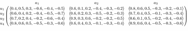
Example 4
Let us consider the decision-making problem given in [41] for bipolar neutrosophic set. “Global environmental concern is a reality, and an increasing attention is focusing on the green production in various industries. A car company is desirable to select the most appropriate green supplier for one of the key elements in its manufacturing process.” [41]. After pre-evaluation, four suppliers(alternatives) are taken into consideration, which are denoted by \(u_1\), \(u_2\), \(u_3\) and \(u_4\). Three criteria are considered including \(a_{1}\) is product quality; \(a_{2}\) is technology capability; \(a_{3}\) is pollution control. Assume the weight vector of the three criteria is \(W=\{w_{1},w_{2},w_{3}\}^{T}=\{0.2,0.5,0.3\}^{T}\). In order to determine the decision information, an expert has gathered the criteria values for the four possible alternatives under bipolar neutrosophic environment. Then
Algorithm
-
Step 1 The decision–making matrix \([b_{ij}]_{m \times n}\) is given by a expert as;
-
Step 2 The positive ideal bipolar neutrosophic solutions for are computed as; \(u^{*}=[\langle 0.8,0.2,0.2,-0.6,-0.3,-0.4\rangle ,\langle 0.9,0.1,0.2,-0.5,-0.2,-0.2\rangle , \langle 0.9,0.1,0.4,-0.5,-0.2,-0.1\rangle ].\)
-
Step 3 The weighted hybrid vector similarity measure between positive ideal (or negative ideal) bipolar neutrosophic solution for alternative \(u_j\in U\) are computed and selected the best alternative.
-
Step 4 Ranking the alternatives (Table 1).

5 Comparative analysis and discussion
In this subsection, a comparative study is presented to show the flexibility and feasibility of the introduced NB-multi-attribute decision-making method. Therefore, different methods are used to solve the same NB-multi-attribute decision-making problem with the bipolar neutrosophic information given by Şahin et al. [36], Deli et al. [18], Deli and Şubaş [16]. Şahin et al. [36] present a method by using Jaccard vector similarity and weighted Jaccard vector similarity measure and Deli and Şubaş [16] present a method by using correlation measure based on multi-criteria decision making for bipolar neutrosophic sets. Also, Deli et al. [18] contains two major phrases. The method firstly use score, certainty and accuracy functions to compare the bipolar neutrosophic sets. Secondly, he use bipolar neutrosophic weighted average operator and bipolar neutrosophic weighted geometric operator to aggregate the bipolar neutrosophic information. The ranking results obtained by different methods are summarized in Table 2.
In Table 2, there are some differences between the ranking results obtained by the methods. The optimal alternative is \(u_{3}\) obtained by the proposed methods except the result obtained by the method of Deli et al.’s method [18] and the proposed method \(HybV_{w}\) with \(\lambda =0.9\). The reason may be score, certainty and accuracy functions and weighted average operator and bipolar neutrosophic weighted geometric operator in Deli et al.’s method [18] and parameter \(\lambda\) in the proposed method \(HybV_{w}\). Generally, the proposed methods can effectively overcome the decision-making problems which contain bipolar neutrosophic information. So, we think the proposed methods developed in this paper is more suitable to handle this application example.
6 Conclusion
This paper developed a multi-criteria decision-making method for bipolar neutrosophic set is developed based on these given similarity measures. To get the comprehensive values, some similarity measures for bipolar neutrosophic sets such as; Dice similarity measure, weighted Dice similarity measure, Hybrid vector similarity measure and weighted Hybrid vector similarity measure are introduced. In the future, it shall be significant to research some special kinds of bipolar neutrosophic measures.
References
Ali M, Smarandache F (2016) Complex neutrosophic set. Neural Comput Appl 25:1–18
Ali M, Deli I, Smarandache F (2016) The theory of neutrosophic cubic sets and their applications in pattern recognition. J Intell Fuzzy Syst 30(4):1957–1963
Atanassov K (1986) Intuitionistic fuzzy sets. Fuzzy Sets Syst 20:87–96
Athar KA (2014) Neutrosophic multi-criteria decision making method. New Math Nat Comput 10(02):143–162
Aydoğdu A (2015) On similarity and entropy of single valued neutrosophic sets. Gen Math Notes 29(1):67–74
Broumi S, Smarandache F (2013) Several similarity measures of neutrosophic sets. Neutro Sophic Sets Syst 1(1):54–62
Broumi S (2013) Generalized neutrosophic soft set. Int J Comput Scie Eng Inf Technol(IJCSEIT) 3/2:17–30
Broumi S, Talea M, Bakali A, Smarandache F (2016) Single valued neutrosophic graphs. J New Theory 10:86–101
Broumi S, Talea M, Bakali A, Smarandache F (2016) On bipolar single valued neutrosophic graphs. J New Theory 11:84–102
Broumi S, Smarandache F, Talea M, Bakali A (2016) An introduction to bipolar single valued neutrosophic graph theory. Appl Mech Mater 841:184–191
Broumi S, Bakali A, Talea M, Smarandache F (2016) Isolated single valued neutrosophic graphs. neutrosophic Sets Syst 11:74–78
Balasubramanian A, Prasad KM, Arjunan K (2015) Bipolar interval valued fuzzy subgroups of a group. Bull Math stat Res 3(3):234–239
Broumi S, Smarandache F (2013) Several similarity measures of neutrosophic sets. Neutrosophic Sets Syst 1(1):54–62
Broumi S, Deli I, Smarandache F (2014) Distance and similarity measures of interval neutrosophic soft sets. In: Critical review, center for mathematics of uncertainty, Creighton University, USA, vol 8, pp 14–31
Broumi S, Deli I (2016) Correlation measure for neutrosophic refined sets and its application in medical diagnosis. Palest J Math 5(1):135–143
Deli I, Subas YA (2016) Multiple criteria decision making method on single valued bipolar neutrosophic set based on correlation coefficient similarity measure. In: International conference on mathematics and mathematics education (ICMME-2016), Frat University, May 12–14, Elazg, Turkey
Chen J, Li S, Ma S, Wang X (2014) m-Polar fuzzy sets: an extension of bipolar fuzzy sets. Sci World J. doi:10.1155/2014/416530
Deli I, Ali M, Smarandache F (2015) Bipolar neutrosophic sets and their application based on multi-criteria decision making problems. In: 2015 International conference on advanced mechatronic systems (ICAMechS). IEEE.(2015, August), pp 249–254
Deli I, Broumi S (2015) Neutrosophic soft matrices and NSM-decision making. J Intell Fuzzy Syst 28:2233–2241
Karaaslan F (2016) Correlation coefficient between possibility neutrosophic soft sets. Math Sci Lett 5(1):71–74
Lee KM (2000) Bipolar-valued fuzzy sets and their operations. In: Proceedings of international conference on intelligent technologies, Bangkok, Thailand, pp 307–312
Lee KJ (2009) Bipolar fuzzy subalgebras and bipolar fuzzy ideals of BCK/BCI-algebras. Bull Malays Math Sci Soc 32(3):361–373
Ma YX, Wang JQ, Wang J, Wu XH (2016) An interval neutrosophic linguistic multi-criteria group decision–making method and its application in selecting medical treatment options. Neural Comput Appl. doi:10.1007/s00521-016-2203-1
Maji PK (2013) Neutrosophic soft set. Ann Fuzzy Math Inf 5(1):157–168
Majumder SK (2012) Bipolar valued fuzzy sets in -semigroups. Math Aeterna 2(3):203–213
Majumdar P, Smanata SK (2014) On similarity and entropy of neutrosophic sets. J Intell Fuzzy Syst 26(3):1245–1252
Mondal K, Pramanik S (2015) Neutrosophic tangent similarity measure and its application to multiple attribute decision making. Neutrosophic Sets Syst 9:85–92
Mukherjee A, Sarkar S (2014) Several similarity measures of neutrosophic soft sets and its application in real life problems. Ann Pure Appl Math 7(1):1–6
Pramanik S, Biswas P, Giri BC (2015) Hybrid vector similarity measures and their applications to multi-attribute decision making under neutrosophic environment. Neural Comput Appl 1–14. doi:10.1007/s00521-015-2125-3
Pramanik S, Mondal K (2015) Cosine similarity measure of rough neutrosophic sets and its application in medical diagnosis. Global J Adv Res 2(1):212–220
Peng JJ, Wang JQ, Zhang HY, Chen XH (2014) An outranking approach for multi-criteria decision–making problems with simplified neutrosophic sets. Appl Soft Comput 25:336–346
Smarandache F (1998) A unifying field in logics neutrosophy: neutrosophic probability, set and logic. American Research Press, Rehoboth
Smarandache F (2005) Neutrosophic set, a generalisation of the intuitionistic fuzzy sets. Int J Pure Appl Math 24:287–297
Santhi V, Shyamala G (2015) Notes On Bipolar-Valued Multi Fuzzy Subgroups Of A Group. Int J Math Arch (IJMA). 6(6). ISSN 2229–5046
Saeid AB (2009) Bipolar-valued fuzzy BCK/BCI-algebras. World Appl Sci J 7(11):1404–1411
Şahin M, Deli I, and Ulucay V (2016) Jaccard vector similarity measure of bipolar neutrosophic set based on multi-criteria decision making. In: International conference on natural science and engineering (ICNASE’16), March 19–20, Kilis
Tian ZP, Wang J, Wang JQ, Zhang HY (2016) Simplified neutrosophic linguistic multi-criteria group decision–making approach to green product development. Group Decis Negot 1–31. doi:10.1007/s10726-016-9479-5
Tian ZP, Wang J, Wang JQ, Zhang HY (2016) An improved MULTIMOORA approach for multi-criteria decision–making based on interdependent inputs of simplified neutrosophic linguistic information. Neural Comput Appl. doi:10.1007/s00521-016-2378-5
Tian ZP, Zhang HY, Wang J, Wang JQ, Chen XH (2015) Multi-criteria decision–making method based on a cross-entropy with interval neutrosophic sets. Int J Syst Sci. doi:10.1080/00207721.1102359
Wang H, Smarandache FYQ, Zhang Q, Sunderraman R (2010) Single valued neutrosophic sets. Multispace Multistructure 4:410–413
Wu J, Cao QW (2013) Same families of geometric aggregation operators with intuitionistic trapezoidal fuzzy numbers. Appl Math Model 37:318–327
Wu XH, Wang JQ, Peng JJ, Chen XH (2016) Cross-entropy and prioritized aggregation operator with simplified neutrosophic sets and their application in multi-criteria decision–making problems. Int J Fuzzy Syst. doi:10.1007/s40815-016-0180-2
Xu X, Zhang L, Wan Q (2012) A variation coefficient similarity measure and its application in emergency group decision making. Syst Eng Proc 5:119–124
Ye J (2014) Vector similarity measures of simplified neutrosophic sets and their application in multicriteria decision making. Int J Fuzzy Syst 16(2):204–215
Ye J (2014) Improved correlation coefficients of single valued neutrosophic sets and interval neutrosophic sets for multiple attribute decision making. J Intell Fuzzy Syst 27:24532462
Ye J, Zhang QS (2014) Single valued neutrosophic similarity measures for multiple attribute decision making. Neutrosophic Sets Syst 2:48–54
Ye S, Ye J (2014) Dice similarity measure between single valued neutrosophic multisets and its application in medical diagnosis. Neutrosophic Sets Syst 6:48–52
Ye J, Fu J (2016) Multi-period medical diagnosis method using a single valued neutrosophic similarity measure based on tangent function. Comput Methods Program Biomed 123:142–149
Ye J (2015) Single-valued neutrosophic similarity measures based on cotangent function and their application in the fault diagnosis of steam turbine. Soft Comput 1–9. doi:10.1007/s00500-015-1818-y
Jun YB, Kang MS, Kim HS (2009) Bipolar fuzzy structures of some types of ideals in hyper BCK-algebras. Sci Math Jpn 70:109–121
Zadeh LA (1965) Fuzzy sets. Inf Control 8:338–353
Zhang HY, Ji P, Wang JQ, Chen XH (2016) A neutrosophic normal cloud and its application in decision–making. Cogn Comput. doi:10.1007/s12559-016-9394-8
Author information
Authors and Affiliations
Corresponding author
Rights and permissions
About this article

Cite this article
Uluçay, V., Deli, I. & Şahin, M. Similarity measures of bipolar neutrosophic sets and their application to multiple criteria decision making. Neural Comput & Applic 29, 739–748 (2018). https://doi.org/10.1007/s00521-016-2479-1
Received:
Accepted:
Published:
Issue Date:
DOI: https://doi.org/10.1007/s00521-016-2479-1