A Gould-type integral of fuzzy functions II

Abstract

In a previous paper, we introduced a new type of integral of a fuzzy function with respect to a real-valued set function. We now provide various specific properties of this new integral, focusing especially on its remarkable continuity properties.

1 Introduction

It is well known that the set-valued integrals are very useful in many theoretical or practical domains like statistics, evidence theory, data mining problems, decision-making theory, subjective evaluations, medicine. Different types of integrals were introduced and studied by many authors. Among them, we remark the Gould integral (Gould 1965), which is defined by using finite Riemann sums for real functions with respect to finitely additive vector measures. The Gould integral was then generalized and studied in Gavriluţ and Petcu (2007a, b), Gavriluţ et al. (2015) (relative to submeasures), Precupanu and Croitoru (2002), Precupanu and Satco (2008) (relative to multimeasures), Gavriluţ (2008), Gavriluţ (2010), Sofian-Boca (2011) (relative to multisubmeasures), Precupanu et al. (2010) (relative to monotone set-valued set functions), Sofian-Boca (2011) (relative to interval-valued set multifunction with respect to the order relation of Guo and Zhang (2004), all for real functions; in [9] for multifunctions; and in Pap et al. (2017), Iosif and Gavriluţ (2017b) for interval-valued multifunction with respect to an interval-valued set multifunction.

Since the non-additive (or fuzzy) measures not always allow modelling many phenomena involving interaction between criteria, Zadeh (1965) introduced the notion of “fuzzy set.” This concept has application in various domains, such as pattern recognition, decision-making under uncertainty, information retrieval, large-systems control and management science. Also, fuzzy integrals (e.g. Choquet, Sugeno integrals) have become an interesting and important topic, with many applications in decision-making problems, information sciences, monotone expectation, aggregation approach, see  Grabisch (1995), Grabisch et al. (1995, 2009), Pham and Yan (1999), Sirbiladze and Gachechiladze (2005), Sugeno (1974), Tsai and Lu (2006).

Nowadays, fuzzy measures are used in the context of aggregation functions, in order to evaluate the relationship among the elements to be aggregated. Aggregation functions are crucial tools to deal with many computation problems. The key property for defining them is monotone increasingness.

On the other hand, interval-valued (set) multifunctions are related to the representation of uncertainty, a necessity coming from economic uncertainty, fuzzy random variables, interval probability, martingales of multivalued functions, interval-valued capacities, interval-valued (intuitionistic fuzzy sets: see, for example, Bykzkan and Duan (2010), Jang (2007), Jang (2012), Jang (2004), Jang (2011), Jang (2006), Tan and Chen (2013), Qin et al. (2016), Bustince et al. (2013) (in multicriteria decision-making problems), Li and Sheng (1998), Weichselberger (2000).

In Iosif and Gavriluţ (2017a), we defined a new type of integral of a fuzzy-valued function (fuzzy function) F relative to a non-negative set function m, by using the Gould method. In this paper, we continue the study of this integral. Section 1 is for introduction. In Sect. 2, we list basic concepts and some results obtained in Iosif and Gavriluţ (2017a) and we also provide some new interesting results. In Sect. 3, we present specific properties of the Gould integral of a fuzzy function relative to a non-negative set function. Also, a study concerning the integrability on atoms is obtained.

2 Preliminaries

${\mathbb {N}}^{*}={\mathbb {N}}\backslash \{0\}.$ If $n\in {\mathbb {N}}^{*}$ , by $i=\overline{1,n}$ we mean $i\in \{1,...,n\}.$ Let be ${\mathbb {R}} _{+}=[0,\infty )$, T a nonempty abstract set and ${\mathcal {A}}$ an arbitrary algebra of subsets of T.

We now recall some notions and remarks that will be used throughout this paper.

Definition 2.1

A finite partition of T is a finite family of nonempty sets $P=\{A_{i}\}_{i=\overline{1,n}}\subset {\mathcal {A}}$ such that $A_{i}\cap A_{j}=\emptyset ,i\ne j$ and $\bigcup \nolimits _{i=1}^{n}A_{i}=T$.

Let be ${\mathcal {P}}$ the class of all partitions of T and ${\mathcal {P}}_{\mathrm {A}}$ the class of all partitions of $\mathrm {A,}$ if $\mathrm {A\in }$${\mathcal {A}}$ is fixed$\mathrm {.}$

Definition 2.2

• (i) If P, $P^{\prime }$$\in {\mathcal {P}}$, $P^{\prime }$ is said to be finer thanP (denoted by $P\le P^{\prime }$ or $P^{\prime }\ge P)$ if every set of $P^{\prime }$ is included in some set of P.

• (ii) The common refinement of two finite partitions $P=$$\mathrm {\{A}_{i}\mathrm {\}}_{i=\overline{1,n}}$ , $P^{\prime }=\{B_{j}\}_{j=\overline{1,m}}$$\in {\mathcal {P}}$ is the partition $P\wedge P^{\prime }=\{A_{i}\cap B_{j}\}_{\begin{array}{c} i=\overline{1,n} \\ j= \overline{1,m} \end{array}}$.

Let be an arbitrary set function $m:{\mathcal {A}}\rightarrow {\mathbb {R}}_{+}$, with $m(\emptyset )=0$ (a boundary condition).

Definition 2.3

Pap (1995) I. m is said to be:

• (i) monotone (or a capacity) (or , fuzzy) if m(A) $\le$m(B), for every $A,B\in {\mathcal {A}}$, with $A\subseteq B$;

• (ii) subadditive if $m(A\cup B)\le m(A)+m(B),$ for every (disjoint) $A,B\in {\mathcal {A}};$

• (iii) a submeasure (in the sense of Drewnowski 1972) if it is monotone and subadditive;

• (iv) null-additive if $m(A\cup B)=m(A)$, for every $A,B\in {\mathcal {A}}$, with $m(B)=0$;

• (v) $\sigma$-subadditive if $m(A)\le \sum \nolimits _{n=0}^{\infty }m(A_{n}),$ for every (pairwise disjoint) $(A_{n})_{n\in {\mathbb {N}}}\subset$${\mathcal {A}}$, with $A=\bigcup \nolimits _{n=0}^{\infty }A_{n}\in ~$${\mathcal {A}}$;

• (vi) finitely additive if $m(A\cup B)=m(A)+m(B),$ for every disjoint $A,B\in {\mathcal {A}};$

• (vii) $\sigma$-additive if $m(\bigcup \nolimits _{n=0}^{\infty }A_{n})=\sum \nolimits _{n=0}^{\infty }m(A_{n})$, for every pairwise disjoint $(A_{n})_{n\in {\mathbb {N}}}\subset {\mathcal {A}}$;

• (viii) order continuous if $\mathop {\hbox {lim}}\nolimits _{{n\rightarrow \infty }} m$($A_{n})=0$, for every decreasing sequence $(A_{n})_{n\in {\mathbb {N}}}\subset {\mathcal {A}}$, with $\underset{n=0 }{\overset{\infty }{\cap }}$$A_{n}=\emptyset ;$

• (ix) exhaustive if $\mathop {\hbox {lim}}\nolimits _{n\rightarrow \infty } m$(${A_{n})=0}$, for every pairwise disjoint sequence $(A_{n})_{n\in {\mathbb {N}}}\subset {\mathcal {A}}$;

• (x) increasing convergent if $\mathop {\hbox {lim}}\nolimits _{n\rightarrow \infty } m$($A_{n})= m(A),$ for every increasing sequence $(A_{n})_{n\in {\mathbb {N}}}\subset {\mathcal {A}}$, with $\underset{n=0}{\overset{\infty }{\cup }}$$A_{n}=A\in {\mathcal {A}}.$

• II. m has the property (S) if for every sequence $(A_{n})_{n\in {\mathbb {N}}}\subset {\mathcal {A}}$, with $\lim \limits _{n\rightarrow \infty }m(A_{n})=0$, there exists a subsequence $(A_{n_{k}})_{k}$ such that $m( {\overline{\mathop {\hbox {lim}}\limits _{k}}} A_{n_{k}})=0$, where ${\overline{\mathop {\hbox {lim}}\limits _{k}}}A_{n_{k}}=\cap \cup A_{n_{k}}.$

• III. A set $A\in {\mathcal {A}}$ is an atom with respect to m if $m(A)>0$ and for every $B\in {\mathcal {A}}$, with $B\subset A$, we have either $m(B)=0$ or $m(A{\setminus } B)=0.$

• IV. m is said to be finitely purely atomic if $T=\bigcup \nolimits _{i=1}^{p}A_{i}$, where $A_{i}\in {\mathcal {A}}$, $i=\overline{1,p}$ are pairwise disjoint atoms of m.

Definition 2.4

• (i) The variation$\overline{m}$ of m is the set function $\overline{m}:{\mathcal {P}}(T)\rightarrow [ 0,+\infty ]$ defined by $\overline{m}(E)=\sup \{\sum \limits _{i=1}^{n}m(A_{i})\}$, for every $E\in {\mathcal {P}}(T)$, where the supremum is extended over all finite families of pairwise disjoint sets $\{A_{i}\}_{i=1}^{n}\subset {\mathcal {A}}$, with $A_{i}\subseteq E$, for every $i=\overline{1,n}$.

• (ii) m is said to be of finite variation on ${\mathcal {A}}$ if $\overline{m}(T)<\infty$.

Remark 2.5

• I. If $E\in {\mathcal {A}}$, then in the definition of $\overline{m}$ one may consider the supremum over all finite partitions $\{A_{i}\}_{i=1}^{n} \mathrm {\in }$${\mathcal {P}}_{E}$.

• II. $\overline{m}$ is monotone on ${\mathcal {P}}(T)$.

• III. If m is finitely additive, then $\overline{m}(A)=m(A),$ for every $A\in {\mathcal {A}}.$

• IV. If m is subadditive ($\sigma$-subadditive, respectively) of finite variation, then $\overline{m}$ is finitely additive ( $\sigma$-additive, respectively) on ${\mathcal {A}}$.

Let be ${\mathcal {P}}_{0}({\mathbb {R}})$ the family of all nonempty subsets of ${\mathbb {R}}$ and ${\mathcal {P}}_{kc}({\mathbb {R}})$ the family of nonempty, compact convex subsets of ${\mathbb {R}}$, i.e. ${\mathcal {P}}_{kc}({\mathbb {R}} )=\{[\underline{a},\overline{a}];\underline{a},\overline{a}\in {\mathbb {R}}, \underline{a}\le \overline{a}\}.$ For $[\underline{a},\overline{a}],[\underline{b},\overline{b}]\in \mathcal {P }_{kc}({\mathbb {R}})$ we define

$$\begin{aligned}{}[\underline{a},\overline{a}]+[\underline{b},\overline{b}]= & {} [\underline{a}+\underline{b},\overline{a}+\overline{b}],\\ \lambda \cdot [\underline{a},\overline{a}]= & {} [\lambda \underline{a},\lambda \overline{a}], \forall \lambda \ge 0. \end{aligned}$$

h is the Hausdorff distance on ${\mathcal {P}}_{0}({\mathbb {R}})$, given by $h(A,B)=\max \{e(A,B),e(B,A)\},$ where $e(A,B)=\sup _{x\in A}d(x,B)$ is the excess of A over B and $d(x,B)=\inf _{y\in B}|x-y|.$

For $[\underline{a},,\overline{a}],[\underline{b},\overline{b}]\in \mathcal {P }_{kc}({\mathbb {R}})$, the Hausdorff distance becomes:

$$\begin{aligned} h([\underline{a},\overline{a}],[\underline{b},\overline{b}])=\max \{| \underline{a}-\underline{b}|,|\overline{a}-\overline{b}|\}. \end{aligned}$$

According to Hu and Papageorgiou (1997), $({\mathcal {P}}_{kc}({\mathbb {R}}),h)$ is a complete metric space.

For every $M\in {\mathcal {P}}_{kc}({\mathbb {R}}),M=[a,b],$ we denote by

$$\begin{aligned} ||M||_{{\mathcal {P}}_{kc}({\mathbb {R}})}=h(M,\{0\})(=\max \{|a|,|b|\}). \end{aligned}$$

If $M\in {\mathcal {P}}_{kc}({\mathbb {R}}_{+}),M=[a,b],$ then $||M||_{{\mathcal {P}} _{kc}({\mathbb {R}})}=b.$

Definition 2.6

A mapping $u:{\mathbb {R}}\rightarrow [0,1]$ is called a fuzzy set on ${\mathbb {R}}.$ For each fuzzy set u, we denote by $[u]^{\alpha }=\{x\in {\mathbb {R}};u(x)\ge \alpha \}$, for every $\alpha \in (0,1]$, its $\alpha$-level set and by $[u]^{0}=\overline{\{x\in {\mathbb {R}} ;u(x)>0\}}$, where, as before, $\overline{A}$ means the closure of the set $A\subseteq {\mathbb {R}}$.

Definition 2.7

A fuzzy set u on ${\mathbb {R}}$ is said to be a fuzzy interval if:

• (i) u is normal, i.e. there exists $x_{0}\in {\mathbb {R}}$ such that $u(x_{0})=1;$

• (ii) u is an upper semi-continuous function;

• (iii) $u(\lambda x+(1-\lambda )y)\ge \min \{u(x),u(y)\},x,y\in {\mathbb {R}} ,\lambda \in [0,1];$

• (iv) $[u]^{0}$ is compact.

Let ${\mathcal {F}}_{C}$ be the family of all fuzzy intervals. For any $u\in {\mathcal {F}}_{C}$, $[u]^{\alpha }\in {\mathcal {P}}_{kc}({\mathbb {R}})$, $\forall \alpha \in [0,1].$ We denote these $\alpha$-levels by $[u]^{\alpha }=[\underline{u}_{\alpha },\overline{u}_{\alpha }],\forall \alpha \in [0,1]$.

For $u,v\in {\mathcal {F}}_{C}$ and $\lambda \in {\mathbb {R}}$, we define:

• the addition $u+v$ and the scalar multiplication $\lambda u$ as follows:

  $$\begin{aligned} (u+v)(x)= & {} \sup _{x=y+z}\min \{u(y),v(z)\};\\ (\lambda u)(x)= & {} u\left( \frac{1}{\lambda }x\right) , \hbox { if }\lambda \ne 0 \hbox { and}\\ \lambda u= & {} \widetilde{0}, \hbox { if } \lambda =0, \hbox { where } \widetilde{0}=\chi _{\{0\}}. \end{aligned}$$

• the order relation $"u\le v"$:

  $$\begin{aligned} u\le v \hbox { iff } u(x)\le v(x),\forall x\in {\mathbb {R}}. \end{aligned}$$

Remark 2.8

• I. If $[\underline{u}_{\alpha },\overline{u}_{\alpha }],[\underline{v} _{\alpha },\overline{v}_{\alpha }]$, $\forall \alpha \in [0,1]$ are $\alpha$-levels of u and v, respectively, the above operations are equivalent to: $[u+v]^{\alpha }=[(\underline{u+v})_{\alpha },(\overline{u+v})_{\alpha }]=[ \underline{u}_{\alpha }+\underline{v}_{\alpha },\overline{u}_{\alpha }+ \overline{v}_{\alpha }]=[u]^{\alpha }+[v]^{\alpha }$ and $[\lambda u]^{\alpha }=[(\underline{\lambda u})_{\alpha },(\overline{\lambda u})_{\alpha }]=[\min \{\lambda \underline{u}_{\alpha },\lambda \overline{u} _{\alpha }\},\max \{\lambda \underline{u}_{\alpha },\lambda \overline{u} _{\alpha }\}],$$\forall \lambda \in {\mathbb {R}}.$ We note that $[\lambda u]^{\alpha }=\lambda [u]^{\alpha }, \forall \lambda \ge 0.$

• II.
  $$\begin{aligned} u\le v\Longleftrightarrow [u]^{\alpha }\subseteq [v]^{\alpha },\forall \alpha \in [0,1]. \end{aligned}$$

We consider the distance on ${\mathcal {F}}_{C}$ defined for every $u,v\in {\mathcal {F}}_{C}$ by

$$\begin{aligned} D(u,v)= & {} \sup _{\alpha \in [0,1]}h([u]^{\alpha },[v]^{\alpha })\\&\left( =\sup _{\alpha \in [0,1]}\max \{|\underline{u}_{\alpha }-\underline{ v}_{\alpha }|,|\overline{u}_{\alpha }-\overline{v}_{\alpha }|\}\right) , \end{aligned}$$

According to Puri and Ralescu (1983), $({\mathcal {F}}_{C},D)$ is a complete metric space.

Let also be $E(u,v)=\sup _{\alpha \in [0,1]}e([u]^{\alpha },[v]^{\alpha }).$

We denote

$$\begin{aligned} \Vert u\Vert _{{\mathcal {F}}_{C}}= & {} D(u,\widetilde{0})\left( =\sup _{\alpha \in [0,1]}h([u]^{\alpha },\{0\}\right) \\= & {} \sup _{\alpha \in [0,1]}\Vert [u]^{\alpha }\Vert _{{\mathcal {P}}_{kc}({\mathbb {R}})}=\sup _{\alpha \in [0,1]}\max \{|\underline{u}_{\alpha }|,|\overline{u}_{\alpha }|\}), \end{aligned}$$

(where $\Vert [u]^{\alpha }\Vert _{{\mathcal {P}}_{kc}({\mathbb {R}})}$ represents the norm induced by h on ${\mathcal {P}}_{kc}({\mathbb {R}})).$

One can easily verify the following properties:

Remark 2.9

• I. $\Vert \cdot \Vert _{{\mathcal {F}}_{C}}$ has the properties of a norm on ${\mathcal {F}}_{C}.$

• II. $D(\lambda u,\lambda v)=|\lambda |\cdot D(u,v),$$\forall u\in \mathcal {F }_{C}$, $\forall \lambda \in {\mathbb {R}}.$

• III. $[\widetilde{0}]^{\alpha }=\{0\},\forall \alpha \in (0,1].$

• IV. $E(u,v)=0\Leftrightarrow u\le v.$

• V. $u\le v\Rightarrow \lambda u\le \lambda v,\forall \lambda \ge 0,\forall u,v\in {\mathcal {F}}_{C}.$

• VI. $u_{1}\le v_{1}$ and $u_{2}\le v_{2}\Rightarrow u_{1}+u_{2}\le v_{1}+v_{2},\forall u_{i},v_{i}\in {\mathcal {F}}_{C},i\in \{1,2\}.$

• VII. $E(u,\widetilde{0})=D(u,\widetilde{0})\Leftrightarrow \{0\}\subseteq [u]^{\alpha },\forall \alpha \in [0,1].$

• VIII. $E(u,\widetilde{0})\le E(u,v)+E(v,\widetilde{0})\le E(u,v)+||v||,\forall u,v\in {\mathcal {F}}_{C}.$

• IX. $u\le v\Rightarrow E(u,\widetilde{0})\le E(v,\widetilde{0}),\forall u,v\in {\mathcal {F}}_{C}.$

• X. $D(u,u+v)\le ||v||,\forall u,v\in {\mathcal {F}}_{C}.$

Definition 2.10

• I. A function $F:T\rightarrow {\mathcal {F}}_{C}$ is called a fuzzy function.

• II. For any $\alpha \in [0,1]$, associated with F, we define the family of interval-valued functions $F_{\alpha }:T\rightarrow {\mathcal {P}} _{kc}({\mathbb {R}})$ by $F_{\alpha }(t)=[F(t)]^{\alpha },\forall t\in T.$

We denote $F_{\alpha }(t)=[\underline{f}_{\alpha }(t),\overline{f}_{\alpha }(t)],t\in T,$ where $\underline{f}_{\alpha },\overline{f}_{\alpha }:T\rightarrow {\mathbb {R}}$ are called the lower, upper functions of F, respectively.

Obviously, $\forall \alpha \in [0,1],\forall t\in T,||F_{\alpha }(t)||_{{\mathcal {P}}_{kc}({\mathbb {R}})}=\max \{|\underline{f}_{\alpha }(t)|,| \overline{f}_{\alpha }(t)|\}.$

In Gavriluţ and Petcu (2007a), we introduced the notions of m-totally measurability and Gould integrability of a real function with respect to a submeasure $m:{\mathcal {A}}\rightarrow {\mathbb {R}}_{+}$, but we may use the same definitions when we deal with a non-negative set function $m:{\mathcal {A}}\rightarrow {\mathbb {R}}_{+}$ with $m(\emptyset )=0.$

Definition 2.11

Gavriluţ and Petcu (2007a) Let $f:T\rightarrow {\mathbb {R}}$ be a real function and $m:{\mathcal {A}}\rightarrow {\mathbb {R}}_{+}$ with $m(\emptyset )=0$.

I. f is said to be $\overline{ m }$-totally measurable (on $(T, {\mathcal {A}},m)$) if for every $\varepsilon >0$, there exists a finite partition $P_{\varepsilon }=\{A_{i}\}_{i=\overline{0,n}}\in {\mathcal {P}}$ such that:

• (i) $\overline{m}(A_{0})<\varepsilon$ and

• (ii) $\text{ osc }(f,A_{i})<\varepsilon , \forall i=\overline{1,n}$, where $\text{ osc }(f,A_{i})= \sup \limits _{t,s\in A_{i}}|f(t)-f(s)|.$

• II. f is said to be $\overline{ m }$-totally measurable on $B\in {\mathcal {A}}$ if the restriction $f|_{B}$ of f to B is $\overline{ m }$-totally measurable on $(B,\mathcal {A_{B}},m_{B})$, where $m_{B}=m|_{{\mathcal {A}}_{B}}$ and ${\mathcal {A}}_{B}=\{A\cap B;A\in {\mathcal {A}}\}$.

We consider $\sigma _{f,m}(P)$ (for short, $\sigma (P))=\sum \limits _{i=1}^{n}f(t_{i})m(A_{i})$, for every $P=\{A_{i}\}_{i= \overline{1,n}}\in {\mathcal {P}}$ and every $t_{i}\in A_{i},i=\overline{1,n}.$

Definition 2.12

Gavriluţ and Petcu (2007a) Let $f:T\rightarrow {\mathbb {R}}$ be a real function and $m:{\mathcal {A}}\rightarrow {\mathbb {R}}_{+}$ with $m(\emptyset )=0$.

• I. f is said to be Gould m-integrable on T if the net $(\sigma (P))_{P\in ( {\mathcal {P}},\le )}$ is convergent in ${\mathbb {R}}.$

  In this case, its limit is called the Gould integral of f on T with respect to m, denoted by $\int _{T}f\mathrm{d}m.$

• II. f is said to be Gould m-integrable on $B\in {\mathcal {A}}$ if $f|_{B}$ is Gould m-integrable on $(B,\mathcal {A_{B}},m_{B})$.

Remark 2.13

• I. If it exists, the integral of f is unique.

• II. f is Gould m-integrable on T if and only if there exists $a\in {\mathbb {R}}$ such that for every $\varepsilon >0$, there exists $P_{\varepsilon }\in {\mathcal {P}}$ so that for every $P=\{A_{i}\}_{i=\overline{ 1,n}}\in {\mathcal {P}}$, with $P\ge P_{\varepsilon }$ and every $t_{i}\in A_{i}$, $i=\overline{1,n}$, we have $|\sigma (P)-a|<\varepsilon .$

Definition 2.14

Iosif and Gavriluţ (2017a) Let be $F:T\rightarrow {\mathcal {F}}_{C}$ a fuzzy function and $m:{\mathcal {A}}\rightarrow {\mathbb {R}}_{+}$ a non-negative set function with $m(\emptyset )=0$.

• I. F is said to be $\overline{ m }$-totally measurable (on$(T, {\mathcal {A}},m)$) if for every $\varepsilon >0$, there exists $P_{\varepsilon }=\{A_{i}\}_{i=\overline{0,n}}\in {\mathcal {P}}$ such that:

• (i) $\overline{m}(A_{0})<\varepsilon$ and

• (ii) $\text{ osc }(F,A_{i})<\varepsilon$, $\forall i=\overline{1,n}$, where $\text{ osc }(F,A_{i})=\sup \limits _{t,s\in A_{i}}D(F(t),F(s))$.

• II. F is said to be $\overline{ m }$-totally measurable on$B\in {\mathcal {A}}$ if $F|_{B}$ is $\overline{ m }$-totally measurable on $(B,\mathcal { A_{B}},\mu _{B})$.

Remark 2.15

• I. Iosif and Gavriluţ (2017a) If F is $\overline{m}$-totally measurable on T, then it is $\overline{m}$-totally measurable on every $A\in {\mathcal {A}}.$ II. (i) $F_{\alpha }$ is $\overline{m}$-totally measurable on T if and only if $\forall \alpha \in [0,1],$ the functions $\underline{f}_{\alpha }, \overline{f}^{\alpha }$ are $\overline{m}$-totally measurable (on T) in the sense of Definition 2.11.

• ii) If F is $\overline{m}$-totally measurable on T, then $\forall \alpha \in [0,1],F_{\alpha }$ is $\overline{m}$-totally measurable on T (in the sense of [9]). In [9], we have the following definition: Let be X a real Banach space, $\mathcal {P}_{0}(X)$ the family of all nonempty subsets of X and $F:T\rightarrow \mathcal {P}_{0}(X)$ a multifunction. F is called $\widetilde{m}$-totally measurable if for every $\varepsilon >0$, there exists $P_{\varepsilon }=\{A_{i}\}_{i=\overline{0,n}}\in {\mathcal {P}}$ such that:

• (i) $\widetilde{m}(A_{0})<\varepsilon$ and

• (ii) $\text{ osc }(F,A_{i})<\varepsilon$, $\forall i=\overline{1,n}$, where $\text{ osc }(F,A_{i})=\sup \limits _{t,s\in A_{i}}h(F(t),F(s))$, where h is the Hausdorff distance on $\mathcal {P}_{0}(X).$

Hence, we can consider that $\forall \alpha \in [0,1],F_{\alpha }$ is $\overline{m}$-totally measurable on T (in the sense of [9]), since $\widetilde{m}$-totally measurability of a multifunction, where $\widetilde{m}(A)=\inf \{\overline{m}(B); A\subseteq B, B \in {\mathcal {A}}\}$, for every $A\subseteq T$, is equivalent to $\overline{m}$-totally measurability by the fact that $\widetilde{m}(A)= \overline{m}(A), \forall A\in {\mathcal {A}}$. Evidently, the converse is not necessarily valid.

We denote $\sigma _{F,m}(P)$ (for short, $\sigma (P))$$=\sum \limits _{i=1}^{n}F(t_{i})m(A_{i})$, for every $P=\{A_{i}\}_{i=\overline{1,n} }\in {\mathcal {P}}$ and every $t_{i}\in A_{i}$, $i=\overline{1,n}$.

Definition 2.16

Iosif and Gavriluţ (2017a) Let be $F:T\rightarrow {\mathcal {F}}_{C}$ a fuzzy function and $m:{\mathcal {A}}\rightarrow {\mathbb {R}}_{+}$ a non-negative set function with $m(\emptyset )=0$.

F is said to be Gouldm-integrable onT if the net $(\sigma (P))_{P\in ({\mathcal {P}},\le )}$ is convergent in $({\mathcal {F}} _{C},D)$. In this case, its limit is called the Gould integral of F on T with respect to $\mu$, denoted by $\int _{T}F\mathrm{d}m.$

Remark 2.17

Iosif and Gavriluţ (2017a)

• I. If it exists, the integral is unique.

• II. If Fm-integrable on T, then $\int _{T}Fd\mu \in {\mathcal {F}}_{C}$. In consequence, F is m-integrable on T if and only if there exists $u\in {\mathcal {F}}_{C}$ such that for every $\varepsilon >0$, there exists $P_{\varepsilon }\in {\mathcal {P}}$, so that for every $P=\{A_{i}\}_{i\in \overline{1,n}}\in {\mathcal {P}}$ with $P\ge P_{\varepsilon }$ and for every $t_{i}\in A_{i}$, $i=\overline{1,n},$ we have $D(\sum \nolimits _{i=1}^{n}F(t_{i})m(A_{i}),u)<\varepsilon .$

Remark 2.18

• (i) For every $\alpha \in [0,1],$

  

  so one immediately has in ${\mathcal {P}}_{kc}({\mathbb {R}})$ that

  $$\begin{aligned} \int _{T}F_{\alpha }\mathrm{d}m=\left[ \int _{T}\underline{f}_{\alpha }\mathrm{d}m,\int _{T}\overline{f} _{\alpha }\mathrm{d}m\right] , \end{aligned}$$

  where $\int _{T}\underline{f}_{\alpha }\mathrm{d}m$ and $\int _{T}\overline{f}_{\alpha }\mathrm{d}m$ are Gould integrals in the sense of Gould (1965).

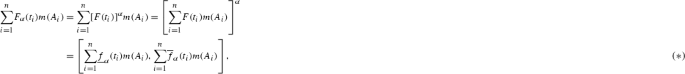
• (ii) Using $(*)$, the definition and the fact that

  $$\begin{aligned}&D\left( \int _{T}F\mathrm{d}m,\underset{i=1}{\overset{n}{\sum }}F(t_{i})m(A_{i})\right) \\&\quad = \underset{\alpha \in [0,1]}{\sup }h\left( \left[ \int _{T}F\mathrm{d}m\right] ^{\alpha },\left[ \underset{i=1}{\overset{n}{\sum }}F(t_{i})m(A_{i})\right] ^{\alpha }\right) \\&\quad =\underset{\alpha \in [0,1]}{\sup }h\left( \left[ \int _{T}F\mathrm{d}m\right] ^{\alpha }, \underset{i=1}{\overset{n}{\sum }}F_{\alpha }(t_{i})m(A_{i})\right) , \end{aligned}$$

  one gets that

  $$\begin{aligned} \left[ \int _{T}F\mathrm{d}m\right] ^{\alpha }=\int _{T}F_{\alpha }\mathrm{d}m\left( =\left[ \int _{T}\underline{f} _{\alpha }\mathrm{d}m,\int _{T}\overline{f}_{\alpha }\mathrm{d}m\right] \right) . \end{aligned}$$
• (iii)
  $$\begin{aligned}&\left\| \int _{T}F\mathrm{d}m\right\| _{{\mathcal {F}}_{C}} =\underset{\alpha \in [0,1]}{\sup }h\left( \left[ \int _{T}F\mathrm{d}m\right] ^{\alpha },\{0\}\right) \\&\quad =\underset{\alpha \in [0,1]}{\sup } \left\| \left[ \int _{T}F\mathrm{d}m\right] ^{\alpha }\right\| _{{\mathcal {P}}_{kc}({\mathbb {R}})} \\&\quad =\underset{\alpha \in [0,1]}{\sup }\max \left\{ \left| \int _{T}\underline{f} _{\alpha }\mathrm{d}m\right| ,\left| \int _{T}\overline{f}_{\alpha }\mathrm{d}m\right| \right\} . \end{aligned}$$

• (iv) Using same argues as before, one immediately has that if F is m -integrable, then for every $\alpha \in [0,1],F_{\alpha }$ is m -integrable (in the sense of [9], i.e. the net $(\sigma _{F_{\alpha },m}(P))_{P\in {\mathcal {P}}}$ is convergent in the Banach space $(\mathcal {P}_{kc}({\mathbb {R}}), h)$, where $\sigma _{F_{\alpha },m}(P)=\sum \limits _{i=1}^{n}F_{\alpha }(t_{i})m(A_{i})$, for every finite partition $P=\{A_{i}\}_{i=\overline{1,n} }\in {\mathcal {P}}$ and every $t_{i}\in A_{i}$, $i=\overline{1,n}.$)

However, this converse and also the converse mentioned in Remark  2.15-II–ii) are valid if one adequately introduces for the family $(F_{\alpha })_{{\alpha \in [0,1]}}$ the corresponding notions of equi-$\overline{m}$-totally measurability and equi-m-integrability.

3 Specific properties of the integral

In this section, we firstly present some continuity properties of the set function $\varphi :{\mathcal {A}}\rightarrow {\mathcal {F}}_{C}$ defined by

$$\begin{aligned} \varphi (A)=\int _{A}F\mathrm{d}m,\forall A\in {\mathcal {A}}, \end{aligned}$$

where, as before, $m:{\mathcal {A}}\rightarrow {\mathbb {R}}_{+}$ is a non-negative set function with $m(\emptyset )=0$ and $F:T\rightarrow {\mathcal {F}}_{C}$ is a fuzzy function which is m-integrable on T (and so, by Proposition 3.9 Iosif and Gavriluţ 2017a, it is m-integrable on every $A\in \mathcal {A }$).

We now recall from Iosif and Gavriluţ (2017a) the following result:

Lemma 3.1

$$\begin{aligned}&\mathrm{(i)}\;D\left( \int _{ T } F\mathrm{d}m, \int _{ T } G\mathrm{d}m \right) \le \underset{t\in T}{\sup }D(F(t),G(T))\cdot \overline{m}(T); \\&(ii)\;||\int _{ T } F\mathrm{d}m ||_{\mathcal {F}_{C}} \le \text { }\underset{t\in T}{\sup } \Vert F(t)\Vert _{\mathcal {F}_{C}} \cdot \overline{m}(T). \end{aligned}$$

Definition 3.2

A set function $\varphi :{\mathcal {A}}\rightarrow {\mathcal {F}}_{C}$ is said to be absolutely continuous with respect tom (denoted by $\varphi \ll m$) if for every $\varepsilon >0$, there is $\delta >0$ such that for every $A\in {\mathcal {A}}$ with $\overline{m} (A)<\delta$, it results $\Vert \varphi (A)\Vert _{\mathcal {F}_{C}} <\varepsilon .$

Definition 3.3

$F:T\rightarrow \mathcal {F}_{C}$ is said to be bounded if there is $M>0$ so that ${\Vert F(t)\Vert _{\mathcal {F}_{C}} \le M}$, for every $t\in T$.

Theorem 3.4

• I. $\varphi \ll m$.

• II. $\varphi$ is finitely additive.

• III. If m is monotone, then the same is$\varphi$.

• IV. If F is bounded and m is of finite variation, then $\varphi$ is of finite variation, too.

Proof

• I. The statement immediately results by Lemma  3.1-(ii).

• II. Evidently, $\varphi (\emptyset )=\widetilde{0}.$ Let be $A,B\in \mathcal { A},A\cap B=\emptyset$ and $\varepsilon >0.$

Since F is m-integrable on A, there exists a partition $P_{A}^{\varepsilon }=\{A_{i}\}_{i=\overline{1,n}}\in {\mathcal {P}}_{A}$ so that for every $P\in {\mathcal {P}}_{A}$, $P\ge P_{A}^{\varepsilon }$, we have

$$\begin{aligned} D\left( \int _{A}F\mathrm{d}m,\sigma (P)\right) <\frac{\varepsilon }{2}. \end{aligned}$$

(1)

Analogously, since F is m-integrable on B, we find a partition $P_{B}^{\varepsilon }=\{B_{j}\}_{j=\overline{1,p}}\in {\mathcal {P}}_{B}$ so that for every $P\in {\mathcal {P}}_{B},$ with $P\ge P_{B}^{\varepsilon },$ we have

$$\begin{aligned} D\left( \int _{B}F\mathrm{d}m,\sigma (P)\right) <\frac{\varepsilon }{2}. \end{aligned}$$

(2)

Now, let be the partition $P_{A\cup B}^{\varepsilon }=\{A_{1},\ldots ,A_{n},B_{1},\ldots ,B_{p}\}\in {\mathcal {P}}_{A\cup B}$. If we consider $P=\{E_{k}\}_{k=\overline{1,q}}\in {\mathcal {P}}_{A\cup B}$ such that $P\ge P_{A\cup B}^{\varepsilon }$ and $t_{k}\in E_{k},k=\overline{1,q}$ then for every $\alpha \in [0,1],$

$$\begin{aligned} \left[ \sum \limits _{k=1}^{q}F(t_{k})m(E_{k})\right] ^{\alpha }&=\left[ \sum \limits _{k=1}^{r}F(t_{k})m(A_{k}^{^{\prime }})\right] ^{\alpha }\\&\quad +\left[ \sum \limits _{k=r+1}^{q}F(t_{k})m(B_{k}^{^{\prime }})\right] ^{\alpha }, \end{aligned}$$

where $\{A_{k}^{^{\prime }}\}_{k=\overline{1,r}}=P_{A}^{^{\prime }}\in {\mathcal {P}}_{A}$ and $P_{A}^{^{\prime }}\ge P_{A}^{\varepsilon }$, $\{B_{k}^{^{\prime }}\}_{k=\overline{r+1,q}}=P_{B}^{^{\prime }}\in {\mathcal {P}} _{B}$ and $P_{B}^{^{\prime }}\ge P_{B}^{\varepsilon }.$

Now, from (1) and (2) we have

$$\begin{aligned}&D\left( \sum \limits _{k=1}^{q}F(t_{k})m(E_{k}),\int _{A}F\mathrm{d}m+\int _{B}F\mathrm{d}m\right) \\&\quad \le D\left( \sum \limits _{k=1}^{r}F(t_{k})m(A_{k}^{^{\prime }}),\int _{A}F\mathrm{d}m\right) \\&\qquad +\,D\left( \sum \limits _{k=r+1}^{p}F(t_{k})m(B_{k}^{^{\prime }}),\int _{B}F\mathrm{d}m\right) <\varepsilon . \end{aligned}$$

So, $\int _{A\cup B}Fd=\int _{A}F\mathrm{d}m+\int _{B}F\mathrm{d}m$ and thus $\varphi$ is finitely additive.

• III. Let be $B,C\in$${\mathcal {A}}$, with $B\subseteq C.$ We prove that in ${\mathcal {F}}_{C}$, $\varphi (B)=\int _{B}F\mathrm{d}m\le \int _{C}F\mathrm{d}m=\varphi (C).$

Since F is m-integrable on B, for every $\varepsilon >0$, there is $P_{\varepsilon }^{1}=\{B_{i}\}_{i=\overline{1,n}}\in {\mathcal {P}}_{B}$ so that for every $P\in {\mathcal {P}}_{B}$, with $P\ge P_{\varepsilon }^{1},$

$$\begin{aligned} D\left( \int _{B}F\mathrm{d}m,\sigma (P)\right) <\frac{\varepsilon }{2}. \end{aligned}$$

(3)

Analogously, there exists $P_{\varepsilon }^{2}=\{C_{j}\}_{j=\overline{1,m} }\in {\mathcal {P}}_{C}$ such that

$$\begin{aligned} D\left( \int _{C}F\mathrm{d}m,\sigma (P)\right) <\frac{\varepsilon }{2}, \end{aligned}$$

(4)

for every $P\in {\mathcal {P}}_{C},$ with$\;P\ge P_{\varepsilon }^{2}.$

If we consider the partition $\widetilde{P}_{\varepsilon }^{1}=\{B_{1},...B_{n},C\backslash B\}$, one can easily check that $\widetilde{P}_{\varepsilon }^{1}\in {\mathcal {P}}_{C}$ and $\widetilde{P} _{\varepsilon }^{1}\wedge P_{\varepsilon }^{2}\in {\mathcal {P}}_{C}$.

Let also be an arbitrary partition $P=\{D_{k}\}_{k=\overline{1,p}}\in {\mathcal {P}}_{C}$, with $P\ge \widetilde{P}_{\varepsilon }^{1}\wedge P_{\varepsilon }^{2}$. We observe that $P_{\varepsilon }^{\prime \prime }=\{D_{k}\cap B\}_{k=\overline{1,p}}\in {\mathcal {P}}_{B}$ and $P_{\varepsilon }^{\prime \prime }\ge P_{\varepsilon }^{1}$. Indeed, since $P\ge \widetilde{P}_{\varepsilon }^{1}\wedge P_{\varepsilon }^{2}$ and $\widetilde{ P}_{\varepsilon }^{1}\wedge P_{\varepsilon }^{2}=\{B_{1},...B_{n},C\backslash B\}\wedge \{C_{j}\}_{j=\overline{1,m} }=\{\{B_{i}\cap C_{j}\}_{\begin{array}{c} i=\overline{1,n} \\ j=\overline{1,m} \end{array}} ,\{C_{j}\backslash B\}_{j=\overline{1,m}}\},$ we get that $P_{\varepsilon }^{\prime \prime }\ge P_{\varepsilon }^{1}$.

Consequently, we have (4) for $\{D_{k}\}_{k=\overline{1,p}}\in {\mathcal {P}} _{C}$ and (3) for $\{D_{k}\cap B\}_{k=\overline{1,p}}\in {\mathcal {P}}_{B}$.

Let $t_{k}\in D_{k}\cap B,k=\overline{1,p}$, be arbitrarily. Then, by (4) and (3) we have

$$\begin{aligned} D\left( \int _{C}F\mathrm{d}m,{}\!\!\sum \limits _{k=1}^{p}F(t_{k})m(D_{k})\right) <\frac{\varepsilon }{2} \end{aligned}$$

and

$$\begin{aligned} D\left( \int _{B}F\mathrm{d}m,{}\!\!\sum \limits _{k=1}^{p}F(t_{k})m(D_{k}\cap B)\right) <\frac{ \varepsilon }{2}, \end{aligned}$$

which imply for every $\varepsilon >0,$

$$\begin{aligned}&E\left( \int _{B}F\mathrm{d}m,\int _{C}F\mathrm{d}m\right) \\&\quad \le D\left( \int _{B}F\mathrm{d}m,{}\!\!\sum \limits _{k=1}^{p}F(t_{k})m(D_{k}\cap B)\right) \\&\qquad +E\left( {}\sum \limits _{k=1}^{p}F(t_{k})m(D_{k}\cap B),{}\!\!\sum \limits _{k=1}^{p}F(t_{k})m(D_{k})\right) \\&\qquad +\,D\left( \int _{C}F\mathrm{d}m,{}\!\!\sum \limits _{k=1}^{p}F(t_{k})m(D_{k})\right) \\&\quad <\varepsilon +\,E\left( {}\!\!\sum \limits _{k=1}^{p}F(t_{k})m(D_{k}\cap B),{}\sum \limits _{k=1}^{p}F(t_{k})m(D_{k})\right) =\varepsilon . \end{aligned}$$

In consequence, $\int _{B}F\mathrm{d}m\le \int _{C}F\mathrm{d}m$.

• IV. Let $\{A_{i}\}_{i=\overline{1,n}}\subset {\mathcal {P}}(T)$ be pairwise disjoint sets and $M=$$\underset{t\in T}{\sup }\Vert F(t)\Vert _{{\mathcal {F}}_{C}} .$ By Lemma  3.1-(ii), it follows $\sum \limits _{i=1}^{n}\Vert \varphi (A_{i})\Vert _{{\mathcal {F}}_{C}} \le M$$\sum \limits _{i=1}^{n}\overline{m}(A_{i})\le M$$\overline{m}(T).$ This implies $\overline{\varphi }(T)\le M$$\overline{m}(T)$, which assures that $\varphi$ is of finite variation. $\square$

Theorem 3.5

If $\overline{m}$ is order continuous (exhaustive respectively), then $\varphi$ is also order continuous (exhaustive respectively).

Proof

The statement easily follows from Lemma 3.1-(ii).

$\square$

Definition 3.6

$\varphi :{\mathcal {A}}\rightarrow {\mathcal {F}}_{C}$ is said to be a D-multimeasure if $\mathop {\hbox {lim}}\limits _{n\rightarrow \infty } D(\varphi (A),\sum \limits _{k=1}^{n}\varphi (A_{k}))=0,$ for every pairwise disjoint sequence $(A_{n})_{n\in {\mathbb {N}}^{*}}\subset {\mathcal {A}}$.

Theorem 3.7

Suppose that $m:{\mathcal {A}}\rightarrow [0,+\infty )$ is a submeasure of finite variation and $F:T\rightarrow$${\mathcal {F}}_{C}$ is bounded.

• I. If m is order continuous (increasing convergent respectively), then $\varphi$ is order continuous (increasing convergent respectively), too.

• II. If m is $\sigma$-additive, then $\varphi$ is a D -multimeasure.

Proof

• I. Since m is order continuous, then by Drewnowski (1972) m is, equivalently, $\sigma$-subadditive, whence $\overline{m}$ is $\sigma$-additive. In consequence, again by Drewnowski (1972), $\overline{m}$ is order continuous, so by Lemma 3.1-(ii), $\varphi$ is order continuous, too.

  Now, suppose m is increasing convergent. Let $\varepsilon >0$ be arbitrary and $(A_{n})_{n\in {\mathbb {N}}^{*}}\subset {\mathcal {A}}$ be so that $A_{n}\nearrow A\in {\mathcal {A}}$.

  Let be $M=\sup \limits _{t\in T}\Vert F(t)\Vert _{{\mathcal {F}}_{C}}$. If $M=0,$ then $F(t)= \widetilde{0}$, for every $t\in T$ and the conclusion is evident. Suppose $M>0$.

  By the additivity of the integral with respect to the set (Theorem 3.4-II), Lemma 3.1-(ii) and Remark 2.9-X), we have:

  $$\begin{aligned}&\displaystyle D(\varphi (A_{n}),\varphi (A)) \nonumber \\&\quad =D\left( \int _{A_{n}}F\mathrm{d}m,\int _{A_{n}}F\mathrm{d}m+\int _{A\backslash A_{n}}F\mathrm{d}m\right) \nonumber \\&\quad \displaystyle \le \Vert \int _{A\backslash A_{n}}F\mathrm{d}m\Vert _{{\mathcal {F}}_{C}} \le M\overline{m} (A\backslash A_{n})\nonumber \\&\quad =M(\overline{m}(A)-\overline{m}(A_{n})). \end{aligned}$$

  (5)

  Now, let $\{B_{i}\}_{i=\overline{1,m}}\subset {\mathcal {A}}$ be an arbitrary partition of A. Then $B_{i}\cap A_{n}\subseteq B_{i}\cap A_{n+1}$, for every $n\in {\mathbb {N}}^{*}$, $i=\overline{1,m}$, and $\bigcup \nolimits _{n=1}^{\infty }(B_{i}\cap A_{n})=B_{i}\cap A=B_{i}$, for every $i=\overline{1,m}$. Since m is increasing convergent, for every $i= \overline{1,m}$, there exists $n_{0}^{i}(\varepsilon )\in {\mathbb {N}}$ so that, for every $n\ge n_{0}^{i}(\varepsilon )$, $m(B_{i})-m(B_{i}\cap A_{n})<\frac{\varepsilon }{2^{i}\cdot M}$.

  Consequently,

  $$\begin{aligned} \sum \limits _{i=1}^{m}m (B_{i})\le & {} \sum \limits _{i=1}^{m}m (B_{i}\cap A_{n})\\&+\quad \,\sum \limits _{i=1}^{m}\frac{\varepsilon }{2^{i}\cdot M}<\overline{m } (A_{n})+\frac{\varepsilon }{M}, \end{aligned}$$

  for every $n\ge n_{0}\text { }{=}\max \limits _{i=\overline{1,m} }\{n_{0}^{i}(\varepsilon )\}.$

  Then $\overline{m}(A)\le \overline{m}(A_{n})+\frac{\varepsilon }{M}$ and by (5), $\varphi$ is increasing convergent.

• II. Let $(A_{n})_{n\in {\mathbb {N}}^{*}}\subset {\mathcal {A}}$ be a pairwise disjoint sequence, with $\bigcup \nolimits _{n=1}^{\infty }A_{n}=A\in {\mathcal {A}}$. Since m is $\sigma$-additive, then it is order continuous, so, by I, the same is true for $\varphi$.

  Because $B_{n}=\bigcup \nolimits _{k=n+1}^{\infty }\!\!\!A_{k}{\searrow } \emptyset$ and $(B_{n})_{n\in {\mathbb {N}}^{*}}\subset {\mathcal {A}},$ there exists $n_{0}(\varepsilon )\in {\mathbb {N}}^{*}$ so that $\Vert \varphi (B_{n})\Vert _{{\mathcal {F}}_{C}} <\varepsilon ,$ for every $n\ge n_{0}(\varepsilon )$.

  Since $\varphi$ is finitely additive, we have

  $$\begin{aligned}&D(\varphi (A),\sum \limits _{k=1}^{n}\varphi (A_{k}))\\&\quad =D\left( \sum \limits _{k=1}^{n}\varphi (A_{k})+\varphi (B_{n}),\sum \limits _{k=1}^{n}\varphi (A_{k})\right) \\&\quad \le \Vert \varphi (B_{n})\Vert _{{\mathcal {F}}_{C}} <\varepsilon , \end{aligned}$$

  for every $n\ge n_{0}$, that is, $\varphi$ is a D-multimeasure. $\square$

Definition 3.8

We say that $\varphi :{\mathcal {A}}\rightarrow {\mathcal {F}}_{C}$has property (S) if for every sequence $(A_{n})_{n\in \mathbb { N}}\subset {\mathcal {A}}$, with $\lim \limits _{n\rightarrow \infty }\varphi (A_{n})=\widetilde{0}$ (with respect to D), there exists a subsequence $(A_{n_{k}})_{k}$ such that $\varphi ( {\overline{\mathop {\hbox {lim}}\limits _{k}}}A_{n_{k}})=\widetilde{0}.$

Theorem 3.9

Suppose that $m:{\mathcal {A}}\rightarrow {\mathbb {R}}_{+}$ is a submeasure of finite variation, which has property (S) and $F:T\rightarrow {\mathcal {F}}_{C}$ is bounded and satisfies the following two conditions:

• (i) $\exists k\in {\mathcal {F}}_{C}$ so that $F(t)\ge k,$ for every $t\in T;$

• (ii) $\{0\}\subseteq [k]^{\alpha }$, for every $\alpha \in {[0,1}].$

  Then$\varphi$has property (S).

Proof

Let be $(A_{n})_{n}\subset {\mathcal {A}}$, with $\lim \limits _{n\rightarrow \infty }\varphi (A_{n})=\widetilde{0}.$ So, for every $\varepsilon >0$, there is $n_{0}(\varepsilon )\in {\mathbb {N}}$, such that for every $n\ge n_{0}(\varepsilon )$, we have

$$\begin{aligned} ||\varphi (A_{n})||_{{\mathcal {F}}_{C}}=\left\| \int _{A_{n}}F\mathrm{d}m\right\| _{{\mathcal {F}}_{C}}<\frac{\varepsilon }{2}. \end{aligned}$$

Since F is m-integrable on each $A_{n}$, for every $\varepsilon >0$ and $n\in {\mathbb {N}}$, there exists $P_{\varepsilon }^{n}=\{A_{i}^{n}\}_{i= \overline{1,m_{n}}}\in {\mathcal {P}}_{A_{n}}$, so that for every $t_{i}^{n}\in A_{i}^{n}$, for $i=\overline{1,m_{n}}$, it holds

$$\begin{aligned} D\left( \sum _{i=1}^{m_{n}}F(t_{i}^{n})m(A_{i}^{n}),\int _{A_{n}}F\mathrm{d}m\right) <\frac{ \varepsilon }{2}. \end{aligned}$$

In consequence,

$$\begin{aligned} \left\| \sum _{i=1}^{m_{n}}F(t_{i}^{n})m(A_{i}^{n})\right\| _{{\mathcal {F}}_{C}}<\varepsilon , \end{aligned}$$

and so, by Remark 2.9, we get

$$\begin{aligned}&||km(A_{n})||_{{\mathcal {F}}_{C}}\\&\quad =m(A_{n})||k||_{{\mathcal {F}}_{C}}=D(km(A_{n}),\widetilde{0})=E(km(A_{n}), \widetilde{0}) \\&\quad \le E\left( k\sum _{i=1}^{m_{n}}m(A_{i}^{n}),\widetilde{0})\right) =E\left( \sum _{i=1}^{m_{n}}km(A_{i}^{n}),\widetilde{0})\right) \\&\quad \le E\left( \sum _{i=1}^{m_{n}}km(A_{i}^{n}), \sum _{i=1}^{m_{n}}F(t_{i}^{n})m(A_{i}^{n})\right) \\&\qquad +\,||\sum _{i=1}^{m_{n}}F(t_{i}^{n})m(A_{i}^{n})||_{{\mathcal {F}}_{C}} <\varepsilon , \end{aligned}$$

which implies $\lim \limits _{n\rightarrow \infty }m(A_{n})=0.$ By the property (S), there exists a subsequence $(A_{n_{k}})_{k}$ of $(A_{n})_{n}$, such that $m({\overline{\mathop {\hbox {lim}}\limits _{k} }}A_{n_{k}})=0.$ Then, we also have $\overline{m}({\overline{\mathop {\hbox {lim}}\limits _{k}}}A_{n_{k}})=0.$

Since

$$\begin{aligned} \left\| \varphi ({\overline{\mathop {\hbox {lim}}\limits _{k} }}A_{n_{k}})\right\| _{{\mathcal {F}}_{C}}= & {} \left\| \int _{ \overline{\lim }A_{n_{k}}}F\mathrm{d}m\right\| _{{\mathcal {F}}_{C}}\\\le & {} \underset{t\in T}{\sup }||F(t)||_{{\mathcal {F}}_{C}}\cdot \overline{ m}\left( {\overline{\mathop {\hbox {lim}}\limits _{k} }}A_{n_{k}}\right) , \end{aligned}$$

we obtain

$$\begin{aligned} \varphi ({\overline{\mathop {\hbox {lim}}\limits _{k}}}A_{n_{k}})=\widetilde{0}. \end{aligned}$$

We now provide some results concerning atoms. In what follows, let T be a locally compact Hausdorff topological space, $\mathcal {K}$ the lattice of all compact subsets of T, $\mathcal {B}$ the Borel $\sigma$-algebra (i.e. the smallest $\sigma$-algebra containing $\mathcal {K}$) and $\mathcal {D}$ the class of all open sets. $\square$

Definition 3.10

A set function $m:{\mathcal {B}}\rightarrow {\mathbb {R}}_{+}$ is called regular if for each set $A\in {\mathcal {B}}$ and each $\varepsilon >0,$ there exist $K\in {\mathcal {K}}$ and $D\in \tau$ such that $K\subseteq A\subseteq D$ and $m(D \backslash K)<\varepsilon .$

In order to state our theorem, we recall Theorem 9.6 Pap (1995).

Theorem 3.11

Let $m:{\mathcal {B}}\rightarrow {\mathbb {R}}_{+}$ be a regular null-additive monotone set function. If $A\in {\mathcal {B}}$ is an atom of m, then there exists a unique point $a\in A$ such that $m(A)=m(\{a\})$.

Corollary 3.12

Let $m:{\mathcal {B}}\rightarrow {\mathbb {R}}_{+}$ be a regular null-additive monotone set function. If $A\in {\mathcal {B}}$ is an atom of m, then there exists a unique point $a\in A$ such that $m(A\backslash \{a\})=0.$

Remark 3.13

Suppose $m:{\mathcal {B}}\rightarrow {\mathbb {R}}_{+}$ is a finitely purely atomic regular null-additive and monotone set function. So there exists a finite family $\{A_{i}\}_{i=1}^{n}\subset {\mathcal {A}}$ of pairwise disjoint atoms of m so that $T=\bigcup \nolimits _{i=1}^{n}A_{i}$. By the above corollary, there are unique $a_{1},a_{2},\ldots ,a_{n}\in T$ such that $m(A_{i}\backslash \{a_{i}\})=0,$ for every $i=\overline{1,n}.$ Then

$$\begin{aligned} m(T\backslash \{a_{1},\ldots ,a_{n}\})\le m(T\backslash \{a_{1}\})+\ldots +m(T\backslash \{a_{n}\})=0, \end{aligned}$$

which implies $m(T\backslash \{a_{1},\ldots ,a_{n}\})=0.$

Now, since m is null-additive, it follows $m(T)=m(\{a_{1},\ldots ,a_{n}\})$.

Theorem 3.14

Suppose $m:{\mathcal {B}}\rightarrow {\mathbb {R}}_{+}$ is a regular null-additive monotone set function and $F:T\rightarrow {\mathcal {F}}_{C}$ be an arbitrary fuzzy function. For every atom $A\in {\mathcal {B}}$, F is m-integrable on A and

$$\begin{aligned} \int _{A}F\mathrm{d}m=F(a)m(A), \end{aligned}$$

where $a\in A$ is the single point resulting by the above theorem.

Proof

Let us consider the partition $P_{0}=\{\{a\},A {\setminus } \{a\}\}.$ Then any fixed partition P of A is of the type $P=\{\{a\},B_{1},\ldots ,B_{p}\},$ with $m(B_{i})=0,\forall i=\overline{1,p}.$ Therefore, $\sigma (P)=F(a)m(\{a\})=F(a)m(A)$. $\square$

Corollary 3.15

Suppose $m:{\mathcal {A}}\rightarrow {\mathbb {R}}_{+}$ is a finitely purely atomic regular null-additive monotone set function, where $T=\displaystyle \cup _{i=1}^{n}A_{i}$ and $\{A_{i}\}_{i=\overline{1,n}}\subset {\mathcal {A}}$ are pairwise disjoint atoms of m. Then any fuzzy function $F:T\rightarrow {\mathcal {F}}_{C}$ is m-integrable on T and

$$\begin{aligned} \int _{T}F\mathrm{d}m=\displaystyle \sum _{i=1}^{n}F(a_{i})m(A_{i}), \end{aligned}$$

where for every $i=\overline{1,n},$$a_{i}\in A_{i}$ is the single point resulting by the above theorem.

References

Bustince H, Galar M, Bedregal B, Kolesarova A, Mesiar R (2013) A New Approach to interval-valued Choquet integrals and the problem of ordering in interval-valued fuzzy set applications. IEEE Trans Fuzzy Syst 21(6):1150–1162
Bykzkan G, Duan D (2010) Choquet integral based aggregation approach to software development risk assessment. Inf Sci 180(3):441–451
Drewnowski L (1972) Topological rings of sets, continuous set functions, integration, I, II, III. Bull Acad Polon Sci Ser Math Astron Phys 20:277–286
Gavriluţ A (2008) A Gould type integral with respect to a multisubmeasure. Math Slov 58:43–62
Gavriluţ A (2010) A generalized Gould type integral with respect to a multisubmeasure. Math Slov 60:289–318
Gavriluţ A, Iosif A, Croitoru A (2015) The Gould integral in Banach lattices. Positivity 19(1):65–82. https://doi.org/10.1007/s11117-014-0283-7
Gavriluţ A, Petcu A (2007a) A Gould type integral with respect to a submeasure. An Şt Univ Al I Cuza Iaşi 53(2):351–368
Gavriluţ A, Petcu A (2007b) Some properties of the Gould type integral with respect to a submeasure. Bul Inst Politehnic din Iaşi Secţia Mat Mec Teor Fiz 53(57):121–130
Gould GG (1965) On integration of vector-valued measures. Proc Lond Math Soc 15:193–225
Grabisch M (1995) Fuzzy integral in multicriteria decision making. Fuzzy Sets Syst 69(3):279–298
Grabisch M, Nguyen HT, Walker EA (1995) Fundamentals of uncertainty calculi with applications to fuzzy inference. Kluwer Academic, Dordrecht
Grabisch M, Marichal JL, Mesiar R, Pap E (2009) Aggregation functions. Cambridge University Press, Cambridge
Guo C, Zhang D (2004) On set-valued fuzzy measures. Inf Sci 160:13–25
Hu S, Papageorgiou N (1997) Handbook of multivalued analysis, vol. I, theory. Mathematics and its applications, vol 419. Kluwer Academic Publishers, Dordrecht
Iosif A, Gavriluţ A (2017a) A Gould type integral of fuzzy functions. Fuzzy Sets Syst. https://doi.org/10.1016/j.fss.2017.08.003
Iosif A, Gavriluţ A (2017b) Integrability in interval-valued (set) multifunctions setting. Bul Inst Politehnic din Iaşi Secţia Mat Mec Teor Fiz 63(67)(1): 65–79
Jang LC (2004) Interval-valued Choquet integrals and their applications. J Appl Math Comput 16:429–445
Jang LC (2006) The application of interval-valued Choquet integrals in multicriteria decision aid. J Appl Math Comput 20(1–2):549–556
Jang LC (2007) A note on the monotone interval-valued set function defined by the interval-valued Choquet integral. Commun Korean Math Soc 22:227–234
Jang LC (2011) On properties of the Choquet integral of interval-valued functions. J Appl Math. https://doi.org/10.1155/2011/492149
Jang LC (2012) A note on convergence properties of interval-valued capacity functionals and Choquet integrals. Inf Sci 183:151–158
Li LS, Sheng Z (1998) The fuzzy set-valued measures generated by fuzzy random variables. Fuzzy Sets Syst 97:203–209
Pap E (1995) Null-additive set functions. Kluwer Academic Publishers, Dordrecht
Pap E, Iosif A, Gavriluţ A (2017) Integrability of an interval-valued multifunction with respect to an interval-valued set multifunction. Iran J Fuzzy Syst. https://doi.org/10.22111/ijfs.2017.3406
Pham TD, Yan H (1999) Color image segmentation using fuzzy integral and mountain clustering. Fuzzy Sets Syst 107(2):121–130
Precupanu A, Croitoru A (2002) A Gould type integral with respect to a multimeasure I/II. An Şt Univ Al.I. Cuza Iaşi 48:165–200/49 (2003), 183–207
Precupanu A, Satco B (2008) The Aumann-Gould integral. Mediterr J Math 5:429–441
Precupanu A, Gavriluţ A, Croitoru A (2010) A fuzzy Gould type integral. Fuzzy Sets Syst 161:661–680
Puri M, Ralescu D (1983) Differentials of fuzzy functions. J Math Anal Appl 91:552–558
Qin J, Liu X, Pedrycz W (2016) Multi-attribute group decision making based on Choquet integral under interval-valued intuitionistic fuzzy environment. Int J Comput Intell Syst 9(1):133–152
Sirbiladze G, Gachechiladze T (2005) Restored fuzzy measures in expert decision-making. Inf Sci 169:71–95
Sofian-Boca FN (2011) Another Gould type integral with respect to a multisubmeasure. An Ştiinţ Univ Al.I. Cuza Iaşi 57:13–30
Sugeno M (1974) Theory of fuzzy integral and applications. PhD Thesis, Tokyo Institute of Technology
Tan C, Chen X (2013) Interval-valued intuitionistic fuzzy multicriteria group decision making based on VIKOR and Choquet integral. J Appl Math. https://doi.org/10.1155/2013/656879
Tsai HH, Lu LY (2006) The evaluation of service quality using generalized Choquet integral. Inf Sci 176:640–663
Weichselberger K (2000) The theory of interval-probability as a unifying concept for uncertainty. Int J Approx Reason 24:149–170
Zadeh LA (1965) Fuzzy sets. Inf Control 8:338–353
Acknowledgements
The authors are indebted to the Area Editor and to the unknown referees for their valuable remarks and suggestions that considerably contributed to the improvement of the paper.
Author information
Authors and Affiliations
Corresponding author
Ethics declarations
Conflict of interest
The authors declare that they have no conflict of interest.
Additional information
Communicated by A. Di Nola.
Rights and permissions
About this article
Cite this article
Gavriluţ, A., Iosif, A. A Gould-type integral of fuzzy functions II. Soft Comput 23, 1099–1107 (2019). https://doi.org/10.1007/s00500-018-3135-8
Published:
Issue Date:
DOI: https://doi.org/10.1007/s00500-018-3135-8