
Abstract
The traditional and still prevailing approach to characterization of flood hazards to dams is the inflow design flood (IDF). The IDF, defined either deterministically or probabilistically, is necessary for sizing a dam, its discharge facilities and reservoir storage. However, within the dam safety risk informed decision framework, the IDF does not carry much relevance, no matter how accurately it is characterized. In many cases, the probability of the reservoir inflow tells us little about the probability of dam overtopping. Typically, the reservoir inflow and its associated probability of occurrence is modified by the interplay of a number of factors (reservoir storage, reservoir operating rules and various operational faults and natural disturbances) on its way to becoming the reservoir outflow and corresponding peak level—the two parameters that represent hydrologic hazard acting upon the dam. To properly manage flood risk, it is essential to change approach to flood hazard analysis for dam safety from the currently prevailing focus on reservoir inflows and instead focus on reservoir outflows and corresponding reservoir levels. To demonstrate these points, this paper presents stochastic simulation of floods on a cascade system of three dams and shows progression from exceedance probabilities of reservoir inflow to exceedance probabilities of peak reservoir level depending on initial reservoir level, storage availability, reservoir operating rules and availability of discharge facilities on demand. The results show that the dam overtopping is more likely to be caused by a combination of a smaller flood and a system component failure than by an extreme flood on its own.
1 Introduction
The traditional and still prevailing approach to characterizing flood hazards to dams is unsuitable for use in risk analysis and assessment for dam safety. This approach assumes that if dams can withstand the effects of the most extreme floods and have generally accepted factors of safety under normal operating conditions they would be safe in an absolute sense (National Research Council 1985). Extreme floods are characterized in terms of the “Inflow Design Flood”, defined in terms of the inflow to the reservoir (either deterministically as the probable maximum flood (PMF) or probabilistically as a flood having a specific probability of occurrence). On the other hand, extreme earthquakes are characterized in terms of the seismic ground motion applied to the dam. Note that while the seismic hazard analysis characterizes the dynamic ground motions as applied to the dam, the flood hazard analysis (i.e. reservoir inflow) does not characterize the dynamic hydraulic forces that are applied to the dam.
This means that in addition to giving a false sense of the safety of dams in terms of the standards-based approach to dam safety assessment, the traditional approach to flood hazard characterization does not provide the necessary information (i.e. magnitude and probability) on the hydraulic forces that are applied to the dam. In fact, within the risk informed dam safety decision framework, the inflow design flood, while essential in establishing the total discharge capacity, is of limited value in the analysis of the hydraulic safety of many dams, no matter how accurately characterized it is. The reason lies in the fact that the reservoir inflow and its associated probability of occurrence is modified by the interplay of a number of factors (initial reservoir level and available storage, reservoir operating rules, various operational faults) on its way to becoming the reservoir outflow and peak level—the two parameters that characterize hydraulic forces acting upon the dam. It is therefore essential to change the approach to flood hazard analysis for dam safety from the currently prevailing focus on reservoir inflows and instead focus on reservoir outflows and corresponding reservoir levels. It should be acknowledged, however, that there are many dams without active discharge control systems and without seasonal fluctuations of their reservoir level where a full pool assumption is not unreasonable. For those kinds of dams the IDF concept could still have its place in dam safety assessment since it is more closely related to resulting peak reservoir level and the probability of dam overtopping. Note that the general focus of the presented study is on dams with seasonally fluctuating reservoir level with active discharge control systems such as gated spillways or low level outlets, since the large majority of high-consequence dams in North America requiring risk-informed approach to dam safety belong to that group.
It should be mentioned that traditional approaches such as the PMF have served the industry well and they still have an important role with respect to design for flood discharge capacity and as the ultimate safety check for capability to pass large floods. However, Hartford and Baecher (2004) pointed out to the potential for increasing risk to the public at lesser events in order to provide protection for the dam at extreme events (i.e. it is not enough to meet the PMF standard without considering the reliability of the gates and power supplies). In the modern context, operational safety during floods less than the design flood, and the matters such as other external system disturbances causing spillway discharge demands over and above the operational discharges, are increasingly important. It is reasonable to assume that in future an increasing number of dam owners will apply some kind of risk informed decision making process in their dam safety assessments regarding natural hazards such as flood. This means that probabilities of reservoir peak outflows and levels will have to be estimated in order to determine probability of dam overtopping and downstream flooding risk. The following examples show that the currently prevailing focus on reservoir inflows in flood hazard analyses for dam safety could be deficient when it comes to risk assessments:
-
Inflow design flood determined as the PMF hydrograph:
-
In most North American jurisdictions (CDA 2007; FEMA 2012), the PMF is typically prescribed as the IDF for high/very high/extreme-consequence dams. After the PMF hydrograph has been derived, it is routed through a reservoir using a set of assumptions and the resulting peak reservoir level is determined. These assumptions vary from place to place and from owner to owner, with the result that all “high-consequence” dams (or high hazard dams) are not equally safe. The peak reservoir level is then used to assess the freeboard and conclude whether or not the dam is safe from overtopping. However, despite being deemed capable of passing the PMF with sufficient freeboard, a given dam may not be as safe as we think due to a number of factors that are typically overlooked in this traditional standard-based approach to flood hazard assessment. Firstly, despite the fact that the theoretical PMF cannot be exceeded, real-life PMF estimates are typically lower than the theoretical upper limit by some variable amount that depends on the available data, the chosen methodology and the analyst’s approach to deriving the estimate (Micovic et al. 2015). Consequently, the exceedance probability of PMF’s reservoir peak outflows and levels is typically greater than zero, could be relatively high in some cases, and remains unknown. The second factor that is typically overlooked is the set of assumptions used in flood routing. It is generally assumed, conservatively, that the PMF occurs on a full reservoir and discharge through the powerhouse is not possible. However, the spillway gates are typically assumed to be fully operable. During an unprecedented natural disaster such as PMF, it is highly likely that some spillway gates would not be operable due to various reasons (power disruption, debris jams, mechanical failures, personnel unavailability, telecommunication problems, etc.).
-
-
Inflow design flood determined as a peak flow having a specific exceedance probability (e.g. 1/10000):
-
Most European jurisdictions do not require the PMF concept and the IDF is derived probabilistically as a peak inflow having a specific probability of exceedance, usually 1/10000 for high-consequence dams (Zielinski 2011). This approach suffers from similar shortcomings as the PMF approach since 1/10000 peak inflow could be associated with an infinite number of hydrographs volumes that will, after reservoir routing, result in peak reservoir level of unknown probability. Generally speaking, floods should always be seen and analyzed in terms of full hydrograph in all studies leading to any type of dam safety assessment. Therefore, it is necessary to convert the peak flow to a flood hydrograph preferably having the same probability of exceedance. This conversion is not straightforward because the peak flow and the flood volume do not necessarily have the same probability of exceedance, since floods could be flashy (i.e. extreme peak, small volume), or have very large volume with no distinct peak. In addition the temporal characteristics of the flood hydrograph timing are also important when it comes to reservoir routing. The same flood volume will produce different maximum reservoir outflow and level when routed, depending whether the flood hydrograph is ‘front-loaded’ (peak appears at the beginning), centre-loaded or end-loaded.
-
In order to obtain the corresponding peak reservoir outflow and peak reservoir level, the hydrograph is routed through the reservoir using a fixed set of assumptions regarding initial reservoir level at the start of the hydrograph as well as regarding various discharge facilities (i.e. availability, start/end of operation, rate of opening/closing). In reality, the initial reservoir level and the discharge facilities availability/way of operation are not constant and their interplay results in exceedance probabilities of reservoir outflow and reservoir levels being different from exceedance probabilities of reservoir inflow.
-
Therefore, no matter how accurate probabilistic characterization of the reservoir inflow is, the probabilities of peak reservoir level remain unknown using ‘inflow design flood’ approach to flood hazard analysis. This practically means that probability of dam overtopping and downstream flooding risk cannot be estimated. There could be a real value in using various stochastic frameworks to better characterise the exceedance probability of inflows, especially in jurisdictions where prescribed probability of inflow is to be satisfied. Such approaches could produce full inflow hydrographs and not just peaks and, with inclusion of reservoir routing in the stochastic model, could yield fairly robust estimates of the probability of overtopping. Unfortunately, in many places, it is still common practice for hydrologists to just develop inflows and pass them over to the hydraulic dam engineers in different departments for the reservoir routing and calculation of corresponding peak reservoir levels. This means that the routing assumptions remain deterministic removing any possibility of getting reasonably accurate probabilistic characterization of the peak reservoir level and consequent risk of dam overtopping.
The inflow design flood (IDF) concept has been and still is being used to size the dam and its designated flood discharge facilities (i.e. spillway, low level outlets) so that the dam could safely pass either a flood of pre-determined probability of exceedance (e.g. 1/10000) or any possible flood (PMF). Note that this concept typically assumes that, during an extreme flood, everything operates according to the plan, i.e. accurate reservoir level measurements, spillway gates open as required, necessary personnel available on site, communication lines fully functioning. In other words, the IDF concept does not address possibility of “operational flood” in which a dam could fail due to a combination of a flood that is much smaller than the IDF and one or more operational faults. The number of possible combinations of unfavourable events causing such a failure is very large and increases with the complexity of the dam or system of dams. Consequently, the probability of dam failure due to an unusual combination of relatively usual unfavourable events, which individually are not safety critical, is larger than the probability of dam failure solely due to an extremely rare flood. Baecher et al. (2013) stated that, for a complex system such as flow control at a dam, the number of possible combinations of unfavorable events is correspondingly as large as the probabilities of any one combination occurring are small. As a result, the chance of at least one pernicious combination occurring can be large. There are many examples of “operational flood” failures, and the two North American examples are illustrated below:
-
Canyon Lake Dam on Rapid Creek in South Dakota failed on June 9th, 1972, resulting in 238 fatalities. The reason for the dam failure was not the lack of flood passing capacity but the inability to use the spillway which was clogged by debris.
-
Taum Sauk Dam in Missouri overtopped and failed on December 14th, 2005. The reason for the overtopping was not high inflow but the error in reservoir level measurement (the pressure transducers that monitored reservoir levels became unattached from their supports causing erroneous water level readings—reporting reservoir levels that were lower than actual levels). In addition, the emergency backup reservoir level sensors were installed too high, thereby enabling overtopping to occur before the sensors could register high reservoir level.
Additional examples of catastrophic dam failures due to failure to open spillway gates as summarized in Gross and Lord (2014) are:
-
Tirlyan Dam, Russia, August 1994 (37 deaths)
-
Belci Dam, Romania, July 1991 (25 deaths)
-
Tous Dam, Spain, October 1982 (20–40 deaths)
Clearly, risk informed decision making in dam safety requires more than the IDF concept which is used to size the dam and spillway for some very large flood under the assumption that everything that happens between inflows entering the reservoir and the reservoir reaching its maximum level, goes according to some predetermined scenario. Many times it does not, as shown above.
In order to have any scientifically-based idea of the probability of dam overtopping due to flood, we should focus on estimating probabilities of peak reservoir level. The process can be described as follows: the reservoir inflow of a certain probability of exceedance is the starting value that gets modified by a complex interplay of starting reservoir level, reservoir operating rules and decisions, and reliability of discharge facilities, personnel and measuring equipment on demand. At the end of the process, the reservoir outflow and associated peak reservoir level have different exceedance probability than the reservoir inflow that started the process. And the exceedance probability of the peak reservoir level is what determines the probability of dam failure due to flood hazard; the exceedance probability of the reservoir inflow is of minor significance in that context.
For example, the latest IDF selection guidelines published by US Federal Emergency Management Agency (FEMA 2013) suggests that besides the traditional prescriptive approach to IDF selection, a risk-informed hydrologic hazard analysis should be carried out at the discretion and judgment of dam safety regulators and owners “for dams for which there are significant tradeoffs between the potential consequences of failure and the cost of designing to the recommended prescriptive standard”. The guidelines suggest that an integral part of risk-informed hydrologic hazard analysis is the development of hydrologic loads that can consist of peak flows, hydrographs, or reservoir levels and their annual exceedance probabilities. Just few months after the publication of FEMA guidelines, US Bureau of Reclamation issued their design standard containing their most recent recommendations for selection of IDF for both existing and new dams (USBR 2013). This USBR design standard is a comprehensive technical document that describes the quantitative risk analysis as “a key aspect of identifying and selecting the IDF” for their dams. Among other things, the USBR document illustrates that the same peak reservoir level could result from very different combinations of peak inflow, inflow volume, and initial reservoir level. It is also interesting to note that, while the PMF concept is still retained as the upper limit of the IDF, the USBR document makes special effort to always use the expression “the IDF or a design maximum reservoir water surface with a design maximum discharge”, thereby implying the importance of the peak reservoir level in the hydrologic hazard analysis.
The peak reservoir level, unlike the reservoir inflow, is not natural and random phenomenon and, consequently, its probability distribution cannot be computed analytically (e.g. by using statistical frequency analysis methods). The probability of the peak reservoir level is the combination of probabilities of all factors leading to it, including reservoir inflows, initial reservoir level, system components failure, human error, measurement error as well as unforeseen circumstances. Thus, the only solution for estimating the probability distribution of the reservoir peak level is some kind of simulation covering as many scenarios as possible. It is a rather complex multi-disciplinary analysis which is currently beyond technical capabilities of some dam owners. However, without it, the proper risk-informed dam safety management is not possible.
There have been various studies attempting to estimate probabilities of dam overtopping with different levels of detail in considering all the contributing factors and possible scenarios. For example, Kwon and Moon (2006) used stochastic simulation to estimate the overtopping probability of a South Korean dam due to flood and wind. The study used a simplified approach of using only annual maxima for precipitation and wind speed to develop flood and wind inputs, and assumed full spillway availability at all times in flood routing through the reservoir. On the other hand, the initial reservoir level input was developed from daily data and it was proven the most sensitive variable in the overtopping probability simulation. Hsu et al. (2011) also attempted to estimate dam overtopping probability induced by flood and wind. The flood input was developed using a fairly simple approach where several frequency distributions were tested on either annual or monthly peak inflows and resulting quantiles were used to develop simple 3-day synthetic inflow hydrographs to be used in reservoir routing. Probably the biggest simplification in this study was the use of constant initial reservoir level in all simulations used to estimate dam overtopping probability. Kuo et al. (2008) also utilized the simplified approach where peak inflows of various exceedance probabilities were converted into hydrographs using the linear concept of unit hydrograph, but considered spillway gate failures in their stochastic simulation and subsequent estimation of dam overtopping risk.
In this paper we present results of stochastic simulation of floods affecting a cascade system of three dams in western Canada, and show the progression from exceedance probabilities of reservoir inflow to exceedance probabilities of peak reservoir level with consideration of initial reservoir level, storage availability, reservoir operating rules and availability of discharge facilities on demand. Section 2 describes the Campbell River hydroelectric system analyzed in this study. Section 3 provides an overview of the stochastic simulation approach including detailed consideration of various hydrometeorological inputs contributing to flood hydrographs, description of complex rules governing the flood routing in a system consisting of three dams and reservoirs, as well as discussion on stochastic simulation of availability of discharge facilities in the system. Section 4 describes specific steps needed to carry out the stochastic simulation described in Sect. 3. The results were presented in Sect. 5, followed by discussion and conclusions in Sect. 6.
2 The Campbell River hydroelectric system
The Campbell River hydroelectric system is located on central Vancouver Island in the province of British Columbia, Canada (Fig. 1). The system consists of three reservoirs. Upper Campbell Lake forms the storage reservoir for the 64 MW Strathcona generating station which discharges into Lower Campbell Lake. Lower Campbell Lake serves as the reservoir for the 47 MW Ladore generating station. Ladore generating station discharges into John Hart Lake, which is the reservoir for the 126 MW John Hart generating station. The total watershed area upstream of Strathcona Dam is 1193 km2. The area for the local watershed between the Ladore and Strathcona dams is 245 km2. The contributing basin area between Ladore and John Hart dams is relatively small at 25 km2. In terms of available reservoir storage, the Strathcona dam reservoir is almost three times larger than the Ladore Dam reservoir, whereas the storage in John Hart Dam reservoir could be considered negligible (i.e. less than 1 % of the Ladore Dam reservoir). The Campbell River System schematic is shown in Fig. 2. The town of Campbell River (population ~30000) is located just 10 km downstream from the John Hart dam. Therefore, the safe operation of the Campbell River System is of critical importance considering the potential catastrophic effects of mis-operation or a failure of the impounding structures.

Location and topography of Campbell River System

Campbell River System schematics (SCA Strathcona; LAD Ladore; JHT John Hart)
3 Overview of the stochastic simulation approach
The basic concept employed in the stochastic approach is the computer simulation of multi-thousand years of flood annual maxima and their progression through the Campbell River System. Stochastic flood modeling was conducted using the Stochastic Event Flood Model (Schaefer and Barker 2001, 2009) in combination with a deterministic precipitation-runoff model, the UBC Watershed Model (Quick 1995; Micovic and Quick 1999). The stochastic event flood model (SEFM) utilizes the UBC watershed model (UBCWM) for conversion of the precipitation input into runoff, and treats the hydrometeorological input parameters as variables instead of fixed values. Monte Carlo sampling procedures are used to allow the climatic and storm-related input parameters to vary in accordance with those observed in nature.
There are three distinct aspects of stochastic flood simulation in such a complex river system. The first aspect is the simulation of natural inflows in each of the three reservoirs within the Campbell River System. The second aspect is the simulation of reservoir operating rules, i.e. flood routing for the individual reservoirs as well as the whole system. Finally, the third aspect is the stochastic simulation of on-demand availability of various discharge facilities within the system, i.e. failure of individual spillway gates, low level outlets, powerhouse outlets, or some combination of those.
All three aspects are combined within the stochastic simulation framework and multi-thousand years of extreme storm and flood annual maxima are generated by computer simulation. The simulation for each year contains a set of climatic and storm parameters that were selected through Monte Carlo procedures based on the historical record and collectively preserved dependencies between the hydrometeorological input parameters. Execution of the UBCWM combined with reservoir routing of the inflow floods through the system and stochastically modelled failure/availability of various discharge gates, provides the computation of a corresponding multi-thousand year series of annual maxima flood characteristics. Characteristics of the simulated floods such as peak inflow, maximum reservoir release, runoff volume, and maximum reservoir level are the flood parameters of interest. An annual maxima series is created for each of these flood parameters and the values are ranked in descending order of magnitude. A non-parametric plotting position formula and probability-plots are used to describe the magnitude-frequency relationships. Note that the stochastic flood model employed here is considered an event model even though the UBCWM is a continuous runoff model. It is termed an event model because each simulation consists of modeling the flood and reservoir response from a specific storm event embedded within the UBCWM continuous simulation period. Thus, each simulation produces one maximum for flood peak discharge, maximum reservoir release, runoff volume, and maximum reservoir level at each of the three dams. These maxima are used in assembling annual maxima series representing multi-thousand years of flood events. Following is a description of each of the three main aspect of stochastic simulation framework.
3.1 Stochastic simulation of reservoir inflows
The UBCWM was used to model hydrological behaviour of the Campbell River System watersheds and simulate inflows to the reservoirs. The model can separately simulate different streamflow components originating from rainfall, snowmelt and glacier melt, and as such is particularly suitable for hydrologic modelling of mountainous watersheds. Since the hydrological behaviour of the mountainous watershed is a function of elevation, the model uses the area-elevation band concept where a watershed is delineated into zones based on elevation, with precipitation and temperature time-series defined for each zone. In terms of the overall structure, the UBCWM has three main analysis modules namely meteorological, soil moisture and routing module (Micovic and Quick 2009). Besides the streamflow calculation, the UBCWM provides information on area of snow cover, snowpack water equivalent, energy available for snowmelt, evapotranspiration and interception losses, soil moisture, groundwater storage, and surface and sub-surface components of runoff. All this information is available for each elevation band separately, as well as for the whole watershed. The physical description of a watershed is input for each elevation band separately in the form of different variables, such as area of the band, forested fraction and forest density, glaciated fraction, band orientation and fraction of impermeable area. Stochastic flood simulation was carried out for inflows to Strathcona (1193 km2 drainage area) and Ladore (245 km2 drainage area) reservoirs. Due to relatively small local area tributary to John Hart reservoir, the local inflow to John Hart was not simulated by the UBCWM but instead estimated by prorating the local inflow to Ladore based on the drainage area ratio of 0.1. Hydrologic calculations are performed on a continuous basis and the UBCWM may be run on either a daily or hourly time step. For this study the UBCWM was calibrated on historically observed data (1983–2014) and run in continuous daily time step mode to establish basin state conditions such as snowpack depth, albedo and soil moisture capacity at the onset of the stochastic storm event. At that point, stochastic storm events were modelled by the UBCWM using an hourly time step and thereby obtaining hourly flood hydrographs.
The hydrometeorological inputs to SEFM and the dependencies that exist in the stochastic simulation of a particular input are listed in Table 1. Note that natural dependencies are prevalent throughout the collection of hydrometeorological variables. The natural dependencies/correlations are preserved in the sampling procedures with a particular emphasis on seasonal dependencies. Sampling of precipitation magnitude over the Ladore watershed is conditioned on the magnitude of precipitation on the Strathcona watershed based on the behavior of historical storms. The sampling of freezing levels is conditioned on both month of occurrence and 24-h precipitation magnitude. The watershed conditions for soil moisture, snowpack, and initial reservoir level are all inter-related and inherently correlated with the magnitude and sequencing of daily, weekly and monthly precipitation. These inter-relationships are established through calibration to historical streamflow records in long-term continuous watershed modelling and the state variables are stored for mid-month and end-of-month conditions. These inter-dependencies are preserved for each flood simulation through the resampling procedure.
Regional analysis methods (Hosking and Wallis 1997) were used in analyzing the characteristics of extreme precipitation. Using this approach, storm data were assembled from all locations that were climatologically similar to the Campbell River watershed. This included assembling precipitation annual maxima series data for the 72-h duration from all stations on Vancouver Island and stations between latitude 47°00′N and 52°00′N from the Pacific Coast eastward to the crest of the Coastal Mountains (Canada) and Cascade Mountains (US). Specifically, annual maxima series datasets were assembled for each station using a calendar year basis that included 72-h precipitation maxima at automated gages and 3-day precipitation at non-recording gages and the dates of occurrence. The 72-h duration (3-day) was selected because it was most representative of the typical storm duration for the Vancouver Island region. Data were obtained from electronic files of Environment Canada, the National Climatic Data Center in the United States and from BC Hydro. This totaled 143 stations and 6609 station-years of record for stations with 25-years or more of record. Detailed description of each of the hydrometeorological inputs from Table 1 as well as the procedures used in stochastic simulation is provided in Micovic et al. (2012). A brief description of the main inputs is provided below.
3.1.1 Storm seasonality
The seasonality of storm occurrence was defined by the monthly distribution of the historical occurrences of 72-h storms with widespread areal coverage that have occurred over Vancouver Island and nearby areas with similar climatic characteristics. This information was used to select the date of occurrence of the storm for a given simulation. The basic concept is that the seasonality characteristics of extraordinary storms used in flood simulations will be the same as the seasonality of the most extreme storms in the historical record.
Storms considered in the analysis were storm events where 72-h precipitation maxima exceeded a 10-year recurrence interval at 3 or more stations. This was done to assure that only storms with both unusual precipitation amounts and broad areal coverage would be considered. This procedure resulted in identification of 69-storm events in the period from 1896 to 2009. A probability-plot was developed using numeric storm dates (9.0 is September 1st, 9.5 is September 15th, 10.0 is October 1st, and so on) and it was determined that the seasonality data could be well described by the normal distribution (Fig. 3). A frequency histogram (Fig. 4) was then constructed based on the fitted normal distribution to depict the twice-monthly distribution of the dates of extreme storms for input into SEFM.

Probability plot of numeric date of occurrence of extreme storms at the 72-h duration for Vancouver Island

Frequency histogram of dates of occurrence of historical 72-h extreme storms for the Campbell River watersheds
A review of Fig. 3 shows historical extreme storms to have occurred in the period from near October 1st through about March 15th with a mean date of December 21st. Flood simulations were conducted using SEFM for mid-month and end-of-month conditions. The probability of occurrence of a storm for any given mid-month or end-of-month can be determined from the incremental bi-monthly probabilities depicted in Fig. 4 (e.g. zero probability for September mid-month, and probability of 0.0228 for September end-month).
3.1.2 Magnitude of 72-h precipitation within extreme storms
Storms for the Strathcona basin are scaled within SEFM by precipitation magnitudes obtained from the 72-h basin-average precipitation-frequency relationship for the Strathcona basin (Fig. 5). This relationship was developed through regional analyses of point precipitation and spatial analyses of historical storms to develop point-to-area relationships and determine basin-average precipitation for the Strathcona basin. Regional L-moment ratios and Kappa distribution parameters (Hosking and Wallis 1997) for the Strathcona basin precipitation-frequency relationship are listed in Tables 2 and 3. The uncertainty bounds were developed through Latin-hypercube sampling method (McKay et al. 1979; Wyss and Jorgenson 1998) where regional L-moment ratios and Kappa distribution parameters were varied to assemble 150 parameter sets and perform Monte Carlo simulation using different probability distributions for individual parameters.

Computed 72-h precipitation-frequency curve and 90 % uncertainty bounds for the 1193 km2 Strathcona basin
Storms for the Ladore basin are scaled within SEFM by precipitation magnitudes obtained from the 72-h basin-average precipitation-frequency relationship for the Strathcona basin. Specifically, the spatial and temporal storm templates are scaled by the ratio of the Ladore to Strathcona basin storm amount for the selected storm.
A comparison of the best-estimate precipitation-frequency relationship with historical storms is shown in Fig. 6. The slope of the best-estimate precipitation-frequency relationship is slightly steeper than the historical values for the Campbell River watershed. This difference can be attributed to natural sampling variability for the shorter record lengths for stations within and near the Campbell River watershed relative to longer record lengths for stations within the regional dataset.

Comparison of best estimate 72-h basin-average precipitation-frequency relationship with historical 72-h precipitation for Strathcona basin
3.1.3 Temporal and spatial distribution of storms
Scalable spatial and temporal storm templates are needed for stochastic generation of storms. A spatial storm template contains the spatial distribution of precipitation over the basin and is made up of the 72-h precipitation amount for each elevation zone, which aggregates to the 72-h basin-average precipitation for the basin. The temporal storm template consists of a collection of dimensionless precipitation mass curves, one mass curve for each elevation zone in the basin. Nine dimensionless precipitation mass curves are needed for the Strathcona basin and five mass curves are needed for the Ladore basin corresponding to the number of modelled elevation zones in each basin for each storm. Construction of the storm templates in this manner allows for scaling of storms to any desired precipitation magnitude and the storm template for a given historical storm is given the name prototype storm.
Stochastic storm generation is accomplished by linear scaling of the spatial and temporal storm patterns for a selected prototype storm. Specifically, the spatial and temporal storm templates are scaled by the proportion of the desired 72-h basin-average precipitation relative to the 72-h basin-average precipitation observed in a selected prototype storm. A brief summary of the process for development of temporal and spatial storm templates can be described as follows:
-
The historical storm record for the Campbell River watershed for the period from 1980 through 2009 was reviewed and 15 storms were identified for use in stochastic modeling of floods. (BC Hydro began comprehensive measurement of hourly precipitation for the Campbell River watershed in the early 1980s.)
-
The 10-day period encompassing each storm of interest was examined and the starting and ending times for the 72-h basin-average precipitation maxima were identified.
-
The spatial storm template for a given storm was developed analyzing hourly rainfall data from point-measurements and using GIS analyses to compute basin-average 72-h precipitation for the Strathcona and Ladore basins and to compute areally averaged 72-h precipitation for each elevation zone. For illustration, the spatial distribution of 72-h precipitation maxima for the October 1984 storm is shown in Fig. 7.
Fig. 7 
Spatial pattern of 72-h precipitation maximum for the October 1984 storm
-
The 10-day period of precipitation encompassing the 72-h precipitation maxima was examined using daily synoptic weather maps, radiosonde data and air temperature temporal patterns. The time span was identified during which there was a continuous influx of atmospheric moisture from the same air mass where precipitation was produced under similar synoptic conditions. This assessment identified the starting and ending times for the precipitation segment that is independent of surrounding precipitation and scalable for stochastic storm generation. Figure 8 depicts the observed 10-day period of basin-average precipitation for the storm of October 14–23, 2003 for the Strathcona basin, with the portion of the hyetograph (in blue) that was identified as the independent scalable segment of the storm and therefore adopted for use as a prototype storm for stochastic storm generation.
Fig. 8 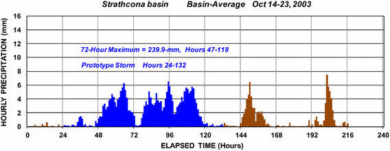
Basin-average temporal pattern for storm of October 14–23, 2003
-
The temporal storm pattern was developed for each elevation zone in the Strathcona and Ladore basins as a weighted-average of hourly precipitation time-series from precipitation stations operating during a given storm. These were stored as dimensionless precipitation mass-curves where the indexing value was the 72-h precipitation maxima for each elevation zone obtained from the spatial storm templates. The collection of dimensionless precipitation mass-curves for the various elevation zones is termed the temporal storm template.


General characteristics of the 15 prototype storms for the Strathcona and Ladore basins are listed in Table 4 showing a considerable diversity among analyzed storms in terms of temporal distribution of precipitation within the 96-h period.
It was mentioned earlier that the 72-h duration is chosen for the frequency analysis as the most representative of the typical storm duration for the studied region. In theory, many durations, especially shorter ones could be included in the frequency analysis in order to examine effects of joint probabilities involved in storms with different characteristics. For example, it is conceivable that a 6-h high-intensity storm, if located over the inundated areas of the catchment, may yield higher reservoir levels than a 72-h storm. However the focus of the study was on Strathcona Dam which has very large reservoir storage and is sensitive to flood volume and is not sensitive to high peak flows that are not supported by a large flood volume. Therefore, the emphasis was on inclusion of longer-duration storm events with larger total volume of precipitation. Furthermore, the suite of 15 scalable storms used in the stochastic analysis includes a diversity of storm events with regard to duration and maximum intensities. The approach taken in modeling was to assemble a collection of storms that were representative of storms on the catchment with regard to both duration and maximum intensity. The representativeness of the suite of storms was demonstrated by assembling probability-plots of depth-duration values for a range of durations from 6-h through 96-h. Two of these plots, for 6/24 and 24/72 h ratios are shown in Fig. 9. These plots demonstrate both the representativeness of the temporal characteristics of the sample of 15 storms and the wide range of storm characteristics in the storm sample.

Probability-plots of depth-duration data for 6/72 and 24/72 h ratios of precipitation maxima for 15 prototype storms for Strathcona basin
3.1.4 Temperature temporal patterns
Temperature temporal patterns are used in computing snowmelt runoff. Scalable temperature temporal patterns were created by first computing hourly time-series for the 1000 mb temperature and freezing level. This was accomplished using land-based hourly air temperature data from the Campbell River Airport, BC Hydro stations located within and near the Campbell River watershed and twice-daily radiosonde temperature measurements from Quillayute, Washington. An example of 1000 mb temperature and freezing level hourly time-series are shown in Fig. 10a for the storm of Oct 14–23, 2003. Resultant air temperature time-series for selected elevations are shown in Fig. 10b along with the basin-average precipitation temporal pattern (Fig. 10c). The temperature temporal pattern for 1000 mb air temperature was created by rescaling the hourly ordinates of the observed 1000 mb temperature time-series by subtracting the 1000 mb index value.

a 1000-mb temperature and freezing level hourly time-series for storm of Oct. 14–23, 2003, b computed temperature time-series for selected elevations during Oct. 14–23, 2003 storm, c precipitation temporal pattern for storm of October 14–23, 2003 (blue-colored storm segment identified for use as prototype storm for stochastic storm generation), and d indexed 1000 mb temperature and freezing level temporal patterns for storm of October 14–23, 2003
The 1000 mb index value is the highest 6-h average 1000 mb temperature observed during the day of maximum 24-h precipitation, which for the storm of Oct 2003 storm was 12.9 °C for the 6-h period from hours 106–111. In a similar manner, the temporal temperature pattern for freezing level was created by rescaling the freezing level hourly time-series by subtracting the index freezing level, which was 3100 m for the Oct 2003 storm. The index freezing level is the average freezing level for the same 6-h period used to compute the temperature index. The indexed 1000 mb temperature and freezing level temporal templates are shown in Fig. 10d. During operation of SEFM, 1000 mb temperature and freezing level time-series are created by reversing the process used to create the temperature temporal templates. Stochastic simulations are used to generate a 1000 mb temperature index value and a freezing level index value for a selected prototype storm. These values are then used to rescale the indexed 1000 mb temperature and freezing level temporal patterns (Fig. 10d) by adding the simulated index values. This yields simulated 1000 mb temperature and freezing level hourly time-series similar to those shown in Fig. 10a. Hourly interpolation between the 1000 mb temperature time-series and freezing level time-series allows air temperature time-series to be computed for each elevation zone.
3.1.5 1000 mb temperature simulation
Temperatures at the 1000 mb level (near sea-level) during extreme storms were simulated using a physically-based probability model for 1000 mb dewpoint temperatures derived from monthly maximum dewpoint data (Hansen et al. 1994). This probability model utilizes end-of-month upper limit dewpoint data and the magnitude of the maximum 24-h precipitation within the storm relative to 24-h PMP. The 1000 mb dewpoint temperatures are drawn from a symmetrical Beta Distribution bounded by lower and upper bounds as depicted in Fig. 11.

Range of 12-h persisting 1000-mb dewpoint temperatures utilized by dewpoint temperature probability model (end-of-December example)
Simulated 1000 mb air temperatures on the day of maximum 24-h precipitation are obtained by adjusting the simulated 1000 mb dewpoint temperature upward by 2 °C. This accounts for relative humidity being near but somewhat less than 100 % as observed in the historical data. The resultant 1000 mb air temperature is then used for scaling of the 1000 mb temperature temporal pattern (e.g. Fig. 10d). The range of possible 1000 mb dewpoint temperatures for a given maximum 24-h basin-average precipitation amount within a storm shown in Fig. 11 indicates that larger storm amounts are generally associated with higher 1000 mb dewpoints. This occurs because high levels of atmospheric moisture are needed to support large precipitation amounts and high levels of atmospheric moisture require higher air temperatures to sustain those moisture levels. A separate relationship, similar to Fig. 11, is used for each end-of-month because 1000 mb dewpoint climatology changes with season. Higher maximum 1000 mb dewpoints are possible in the fall months of October and November than in the colder winter months of January and February. Thus, freezing levels tend to be somewhat lower for storms in the colder winter months.
3.1.6 Air temperature lapse-rates
Air temperature lapse-rates are used in the stochastic modeling of freezing levels. Analyses of data from Quillayute WA and Oakland CA found that air temperature lapse-rates on the day of maximum 24-h precipitation for noteworthy storms were well described by the Normal Distribution (Fig. 12). The mean value was found to be 5.1 °C/1000 m, which is near the saturated pseudo-adiabatic lapse-rate. Similar results were found if examining the data from Quillayute WA or Oakland CA separately and the data from the two stations were combined to provide a larger sample for computing the distribution parameters.

Air temperature lapse-rates for day of maximum 24-h precipitation for storms near Southwestern BC and Central California
3.1.7 Freezing level
Freezing level on the day of maximum 24-h precipitation is used for scaling the freezing level temporal pattern (e.g. Fig. 10d). Simulations are conducted by stochastically generating a 1000-mb air temperature as described above, selecting an air-temperature lapse-rate from the Normal distribution depicted in Fig. 12 and computing the resulting freezing level. The computed freezing level is then used to scale the freezing level temporal pattern by adding the value of the computed freezing level to the indexed temporal pattern.
Figure 13 shows an example of 600 computer simulations of freezing level, which shows moderate variability in freezing level with storm magnitude. The behaviour of freezing level for extreme storms adds some non-linearity to the flood response in that higher temperatures and larger snowmelt contributions are associated with larger precipitation amounts.

Example of variability in simulation of freezing level including variability due to 1000 mb air temperature and air temperature lapse-rate
3.1.8 Watershed model antecedent condition sampling
A resampling approach was used to determine the model state variables (initial snowpack, soil moisture conditions, and initial streamflow) at the onset of a stochastically generated storm. As previously mentioned the UBCWM was used to continuously simulate daily streamflow from October 1983 to present time. Model state variables were saved at the middle and the end of each month during the simulation using a feature in the UBCWM that saves all relevant model variables and antecedent conditions allowing for the model to restart at that time without re-running the previous period. This provided a total of 32-years of antecedent conditions on a twice-monthly basis for resampling. UBCWM state variables were randomly selected from one of the 32-years for the date of storm occurrence. Each year was equally-likely to be chosen using the resampling approach.
3.1.9 Initial reservoir level
The reservoir level for John Hart Dam varies little throughout the year and was set to a constant value of 139.28 m at the beginning of each simulation, which represents the mean elevation for the period of record. A resampling approach was used to determine the reservoir elevation at the beginning of the simulation for Strathcona and Ladore Dams. Reservoir operating rules, especially in such a complex system such as Campbell River System, typically change over time due to various reasons. Therefore it is important to resample reservoir level data only from the period in historic record that reflects current system/reservoir operating rules. For the Campbell River System that period included reservoir level data from January 1998 through to the present. The current system/reservoir operating rules were established in 1998 with the goal to find a compromise among the needs of various stakeholders. As a result, hydropower operation, environmental constraints and recreational demands limit the reservoir operating range. An attempt was made to use reservoir inflow data available since 1960s as an input to the reservoir operation optimization model and derive a longer record of synthetic reservoir levels. However the derived synthetic reservoir levels when compared with the recorded reservoir levels for the same post-1998 period exhibited smaller range between maximum and minimum elevation than the recorded level data. This is due to the fact that the optimization model makes operating decisions (spill, store, generate) on the perfect inflow foresight, whereas in the real-life operations the inflow forecast is uncertain and operating decisions made under inflow uncertainty result in higher maximum and lower minimum levels. Thus, for this study it was decided to use recorded reservoir levels reflecting the current operating rules despite very short record length. Since the reservoir resampling period was different (shorter) from the UBCWM antecedent condition sampling period, it was necessary to ensure that the year selected for reservoir level resampling had similar seasonal moisture and runoff characteristics as the year selected for the UBCWM antecedent conditions. This was accomplished by selecting the reservoir levels from years with similar antecedent precipitation as the year selected for the UBCWM antecedent conditions.
3.2 Simulation of reservoir operation during flood
Flood routing simulations were carried out with the aim to realistically capture the way the Campbell River System may be operated during flood events ranging in their exceedance probabilities from 1/10 to beyond 1/10000. In reality this is a rather complex decision making process involving consultations amongst several functional units including operations, dam safety and site facilities. Typically the flood routing decisions are based on the inflow forecast and flood magnitude, downstream environmental conditions existing at the time of the inflow, and other site-specific and date-specific conditions. For example, in order to minimize flooding of the town of Campbell River situated downstream of the Campbell River Hydroelectric System, the total system discharge is limited to 700 m3/s during the times when the most upstream reservoir (Strathcona) is below El. 222.0 m (when the reservoir rises above that level, dam safety takes precedence over downstream flooding and the discharge is set equal to the lower of the inflow or the maximum discharge capacity). The complicating fact is that streamflow from the 278 km2 Quinsam River basin contributes to the Campbell River streamflow between the most downstream dam (John Hart) and the town of Campbell River. This means that most of the time, the system release is dependent on Quinsam River unregulated streamflow. The flood routing procedures for the entire Campbell River System are incorporated into SEFM framework as shown in Table 5.
3.3 Stochastic simulation of the availability of discharge facilities
Generally, the reservoir routing of an extreme flood in dam safety analyses is performed by assuming a conservatively high initial reservoir level combined with the (non-conservative) assumption that all spillway gates open as required to pass flood discharge. Some analyses assume the “n-i” rule where “n” is the number of spillway gates and “i” is the number of spillway gates assumed unavailable. However, depending on values for “n” and “i”, this approach may be unrealistically conservative for some spillway configurations.
Each of the three Campbell System dams has a three-bay gated spillway, totalling nine spillway gates for the entire system. The spillway capacities are fairly similar with total discharge capacity at the dam crest elevation being 1500, 1600 and 1650 m3/s, for Strathcona, Ladore and John Hart dams respectively. During the passage of a flood, one or more of those nine gates may be unavailable for various reasons including debris jams, human error and mechanical or electrical malfunctions. An international survey of incidents regarding various components of spillway gate systems (Hobbs 2003) indicated that human factors and the failure of protection systems (limit switches, controls, position indicators, etc.) account for the highest number of incidents, whereas hoist units have surprisingly few incidents. Due to numerous interconnected components of a spillway gate system and consequently the infinite number of reasons for failure, it is impossible to directly compute the probability of gate failure on demand. This probability has to be estimated through some kind of analysis which should include as many failure modes as possible, with consideration of site-specific knowledge of the state of various gate system components as well as frequency and thoroughness of gate testing. One example of such analysis was carried out during gate reliability assessments of five US Army Corps of Engineers Huntington District dams (Lewin et al. 2003). Gate and equipment testing for these five dams of three to four times per year was considered relatively infrequent. In addition, many components, such as relays or limit switches were tested only when the gate test used those particular components. During 18 gate tests, there were three instances when a gate failed to operate correctly. A fault tree analysis of gate failure modes indicated that for a gate opening in ideal conditions, similar to those under which gate tests were carried out, a probability of failure on demand was assessed to be of the order of 1 in 10 (0.1). The probability of multiple failures of gates during an extreme flood was estimated to be at least 1 in 100 (0.01) per demand due to a common cause failure regardless of the number of gates in an installation. The authors indicated that their estimates should be examined in more detailed reliability studies.
In the present study, we developed failure likelihood functions for each spillway gate in the system based on qualitative analyses and consultations among engineers involved in BC hydro-wide gate reliability program as well as in maintenance and testing of the Campbell System spillway gates. The factors considered were conditions of individual components of the spillway gate system (both mechanical and electrical), maintenance schedule, potential failure modes, human factors and frequency of gate testing (monthly in this case). All combinations (one, two or three out of three gates failing to open) were considered, along with the probability of fixing failed gates and bringing them back in service within a 12-h period. The estimated probabilities of Campbell System spillway gates failing to open (per demand) are presented in Table 6.
Note that the probability of two gates failing at the same time is very similar to that of three gates failing together. This is due to the assumption that the most likely cause for the joint failure of multiple gates is power supply.
The availability of powerhouses during flood is uncertain. Flood-inducing rainfall could be very severe and could conceivably cause erosion or landslides that might result in transmission line failures, making generation impossible. Severe rainfall could also cause other powerhouse-disabling damage such as powerhouse flooding or penstock damage. Perhaps the most realistic way of simulation would be to somehow tie the availability of the powerhouse to the storm magnitude (e.g. if the simulated 72-h basin-average precipitation has the exceedance probability of 1/1000 or less, the powerhouse discharge is disabled). However, considering that the maximum powerhouse discharges at all three Campbell System power plants represent very small fraction of the total flood discharge (about 10 % of 100-year flood, and less than 4 % of the PMF), proper simulation of powerhouse availability has minor effect on the final flood routing results. Thus in order to simplify the simulation, this study used the conservative assumption of all three powerhouses being unavailable for flood discharge.
4 Simulation procedure
Flow charts for the stochastic simulation procedure for the Campbell River System are shown in Figs. 14 and 15.

Flow chart for stochastic simulation procedure to derive inflows to Strathcona and Ladore reservoirs (Steps 1–4)

Flow chart for stochastic simulation procedure to derive outflows and peak reservoir levels for each dam in Campbell River System (Steps 1–5)
As mentioned earlier, the stochastic flood modeling was done on Strathcona and Ladore watersheds only. Local inflow to the John Hart reservoir was not simulated by the UBCWM but instead was estimated by prorating the local inflow to Ladore based on the drainage area ratio of 0.1. The entire stochastic simulation procedure can be grouped into five principal steps:
Step 1—Select date of storm occurrence:
-
Select mid-month or end-of-month date for storm occurrence based on historical seasonality of storm occurrences
Step 2—Select all parameters associated with the occurrence of the storm event:
-
Select the magnitude of the 72-h precipitation for Strathcona basin based on 72-h basin-average precipitation-frequency relationship for Strathcona basin
-
Select the magnitude of the 72-h precipitation for Ladore basin based on 72-h basin-average precipitation-frequency relationship for Ladore basin
-
Select one of 15 prototype storms for describing the temporal and spatial distribution of the storm, and scale the prototype storm templates to have the selected 72-h basin-average precipitation amount
-
Select 1000 mb air temperature from a physically-based probability temperature model for the day of maximum 24-h precipitation in selected prototype storm
-
Select air-temperature lapse-rate and compute reference freezing level for day of maximum 24-h precipitation for selected prototype storm based on 1000 mb air temperature and air temperature lapse-rate
-
Compute temporal temperature patterns using scaled 1000 mb air temperature and freezing level temporal patterns for selected prototype storm and compute hourly temperature time-series for all elevation zones
Step 3—Establish antecedent watershed and reservoir conditions at onset of storm:
-
Select UBCWM antecedent condition file for mid-month or end-of-month that was selected for the occurrence of the storm. This is selected from the antecedent condition files created from the long-term continuous simulation of the UBCWM (Oct/1983–present). This sets the antecedent snowpack, soil moisture, and other model state variables.
-
Select initial reservoir level for Strathcona and Ladore reservoirs. This is sampled from recorded reservoir level data for the period 1/1/1998–present. The sampled year has similar antecedent precipitation as the year sampled for the UBCWM antecedent conditions. The sampled month and day corresponds to a 15-day period surrounding the sampled mid-month or end-of-month (7-days before and 7-days after selected date). The initial reservoir level for John Hart Dam reservoir was constant for each simulation because the reservoir level varies little throughout the year and from year to year.
Step 4—Conduct watershed modeling for each dam:
-
Conduct rainfall-runoff and snowmelt modeling using the UBCWM. Computed reservoir inflows are saved for each simulation.
Step 5—Conduct reservoir routing of inflow floods:
-
Execute reservoir routing that incorporates all reservoir operational procedures as well as spillway gate failure likelihood functions. Routing is performed separately for each dam with all inflows routed in batch for each dam. Routing starts with the most upstream dam (Strathcona) and proceeds with each subsequent dam downstream.
The Monte Carlo simulation procedure carried out for Strathcona basin with all steps involved is illustrated in Fig. 16.

Monte Carlo simulation sequence for Strathcona basin
5 Results
The results from the Monte Carlo stochastic simulations were used to develop magnitude-frequency relationships for reservoir elevation, peak inflow, peak outflow, and 72-h reservoir inflow volume for each dam in the Campbell River system. These relationships were based on 100000 computer simulations using a variation of Latin-hypercube censored sampling (McKay et al. 1979; Wyss and Jorgenson 1998) for the precipitation input that allowed the flood-frequency curves to be developed in a piecewise manner. This greatly reduced the number of simulations that would otherwise have been required to develop the flood-frequency relationships.
The results are presented as probability-plots using standard plotting position methods (Stedinger et al. 1992). This approach avoids difficulties of selecting and fitting a probability distribution to model outputs. Outputs from the stochastic flood model were ranked in descending order of magnitude and the estimate of the annual exceedance probability for each ranked flood output was obtained from the Cunnane plotting position formula (Cunnane 1978) using Gringorten weighting factor of 0.44.
Reservoir inflow, outflow, 72-h inflow volume and elevation magnitude-frequency plots for Strathcona Dam are shown in Fig. 17.

Strathcona dam: magnitude-frequency plot for hourly peak reservoir inflow, outflow and elevation, and 72-h inflow volume
The entire Monte Carlo stochastic simulations process was repeated with addition of random spillway gate failures incorporated into reservoir routing. Note that the purpose of this analysis was to illustrate the importance of considering spillway gate reliability and the gate failure probabilities described in Sect. 3.3 are essentially notional. Those numbers are highly site-specific, and even if rigorously analyzed can be expected to have wide (order of magnitude) uncertainty bounds. Magnitude-frequency plots for reservoir elevation comparing cases with and without spillway gate failures for all three dams are shown in Figs. 18, 19, and 20.

Strathcona dam: magnitude-frequency plot for 1-h peak reservoir elevation with and without spillway gate failures

Ladore Dam: magnitude-frequency plot for 1-h peak reservoir elevation with and without spillway gate failures

John Hart Dam: magnitude-frequency plot for 1-h peak reservoir elevation with and without spillway gate failures
6 Discussion and conclusions
The aim of this study was to address the widely used concept of Inflow Design Flood (IDF) and evaluate its adequacy in the dam safety context. IDF is a necessary parameter for sizing the surcharge storage, height of a dam and outlet works, and could be useful in assessing safety of dams with fairly steady reservoir level (where a full pool assumption is not unreasonable) and dams without active discharge control systems. However, in regard to individual dams or dam systems with fluctuating reservoir elevation and active discharge control systems such as gated spillways or low level outlets, the IDF concept is inadequate for use in any flood hazard risk assessment analyses for dam safety. For those types of dams and dam systems, the IDF, by characterizing inflow to the reservoir, does not provide the necessary information (i.e. magnitude and probability) on the flood hazard in terms of hydraulic forces acting on the dam itself (peak reservoir level). The commonly used solution for this problem is to route the IDF through the reservoir and determine the resulting peak reservoir level, and thereby obtain at least some information (magnitude but not probability) on the flood hazard acting on the dam. However, it is important to point to serious shortcomings of such an approach that can lead to false sense of the safety of dams and the belief that dams are safer than they actually are.
It should be noted that many jurisdictions currently use a standard-based approach and require that IDF be determined either as the PMF or a peak flow of some specific probability of exceedance. In the latter case, it would still be advantageous to utilize some kind of stochastic method even though the estimation of a specific standard does not require considering risks over the full probability domain.
This paper presents the alternative where, for a system of three dams with fluctuating reservoir elevation and active discharge control systems, the focus of flood hazard analysis for dam safety was shifted from reservoir inflows to reservoir outflows and corresponding reservoir levels. The full probability domain of the peak reservoir level is derived as the combination of probabilities of all factors leading to it, including reservoir inflows, initial reservoir level, system components failure, human error, measurement error as well as unforeseen circumstances, and could be estimated through some kind of stochastic simulation covering as many scenarios as possible. The results of such a simulation on the Campbell River System show that dams are much more likely to be overtopped (and consequently fail) due to an unusual combination of otherwise somewhat common individual events than due to a single extreme flood event (e.g. the 72-h PMF inflow volume to Strathcona of 840 million m3 has annual exceedance probability of well beyond 10−7, according to the frequency curve in Fig. 17). It can also be concluded that the importance of spillway gate reliability increases as the size of available surcharge storage decreases. For example, in the Strathcona Dam case, spillway gate failure would not have any effect on the probability of dam overtopping due to both large surcharge storage and the existence of Low Level Outlet which can discharge equivalent of almost two spillway gates. However, in the case of John Hart Dam, where the available surcharge storage is practically negligible, simulating possibility of spillway gate failures during the flood increased the resulting probability of dam overtopping by five orders of magnitude over the case in which all spillway gates are assumed operable.
It should be mentioned that, beside spillway gate failures, there are many other things that could go wrong during the flood (e.g. human error in reservoir operations, telemetry errors, landslides into reservoir, debris, etc.) not considered in the presented simulation. Accounting for those factors will further increase probability of dam overtopping.
Also note that there are numerous uncertainties associated with the type analysis carried out in this study. For instance the estimated probabilities of spillway gate failures per demand may appear too low or too “optimistic” to some. Increasing these probabilities would lead to increased probability of dam overtopping. Also, estimates of exceedance probability of extreme floods (i.e. 10−4 and less) with relatively small amount of observed hydrometeorological data are inherently uncertain. If the SEFM/UBCWM modelling framework and methodology it utilizes was replaced by another stochastic simulation method used for estimating extreme flood probabilities (e.g. Nathan and Weinmann 2003; Paquet et al. 2013), the magnitude-frequency results would likely be somewhat different, especially for rare events. However, regardless of inevitable uncertainties in the final results arising from lack of observed data, input assumptions and methodological choices, the biggest value of this study is that it quantifies the relative difference in dam safety level between the case when every discharge facility operates as required, and the more realistic case in which some discharge facilities occasionally fail to operate.
Finally, the presented results may have appearance of “bad news” since they show that in some cases our perception of dam safety is wrong and we start to realize that our dams are not as safe as we previously thought. However, it is much better to be aware of a problem and start working on it (thorough analysis of as many as possible failure modes within the dam/reservoir system, potential modification of reservoir operating rules to minimize impact of gate failures to dam safety, increased maintenance and testing of discharge facilities leading to improved operational reliability, emergency preparedness/planning) than to believe that there is no problem and be surprised when dam designed to pass the prescribed IDF overtops and fails during a flood that is much smaller than the IDF.
References
Baecher GB, Hartfor DND, Patev RC, Rytters K, Zielinski PA (2013) Understanding spillway systems reliability. In: Proceedings of ICOLD 81st annual symposium, Seattle, pp 1241–1250
CDA (2007) Dam safety guidelines. Canadian Dam Association, Edmonton
Cunnane C (1978) Unbiased plotting positions—a review. J Hydrol 37:205–222. doi:10.1016/0022-1694(78)90017-3
FEMA (2012) Summary of existing guidelines for hydrologic safety of dams, FEMA report P-919
FEMA (2013) Selecting and accommodating inflow design floods for dams, FEMA report P-94
Gross E, Lord DW (2014) Why are dams failing before they reach their spillway design capacity? In: Proceedings of the 34th annual USSD conference, San Francisco
Hansen EM, Fenn DD, Corrigan P, Vogel JL, Schreiner LC, Stodt RW (1994) Probable maximum precipitation for Pacific Northwest States—Columbia River (including portions of Canada), Snake River and Pacific coastal drainages, hydrometeorological report No. 57, US National Weather Service, Silver Spring
Hartford DND, Baecher GB (2004) Risk and uncertainty in dam safety. Thomas Telford Publishing, London
Hobbs G (2003) Spillway gates—a survey of operational and reliability issues. Paper presented at 2003 ANCOLD conference, Hobart
Hosking JRM, Wallis JR (1997) Regional frequency analysis—an approach based on L-moments. Cambridge University Press, Cambridge
Hsu YC, Tung YK, Kuo JT (2011) Evaluation of dam overtopping probability induced by flood and wind. Stoch Env Res Risk Assess 25(1):35–49. doi:10.1007/s00477-010-0435-7
Kuo JT, Hsu YC, Tung YK, Yeh KC, Wu JD (2008) Dam overtopping risk considering inspection program. Stoch Environ Res Risk Assess 22(3):303–313. doi:10.1007/s00477-007-0116-3
Kwon HH, Moon YI (2006) Improvement of overtopping risk evaluations using probabilistic concepts for existing dams. Stoch Environ Res Risk Assess 20(4):223–237. doi:10.1007/s00477-005-0017-2
Lewin J, Ballard G, Bowles DS (2003) Spillway gate reliability in the context of overall dam failure risk. In: Proceedings of the 23rd annual USSD conference, Charleston, ISBN: 9781884575327
McKay MD, Conover WJ, Beckman RJ (1979) A comparison of three methods for selecting values of input variables in the analysis of output from a computer code. Technometrics 21:239–245
Micovic Z, Quick MC (1999) A rainfall and snowmelt runoff modelling approach to flow estimation at ungauged sites in British Columbia. J Hydrol 226:101–120. doi:10.1016/S0022-1694(99)00172-9
Micovic Z, Quick MC (2009) Investigation of the model complexity required in runoff simulation at different time scales. Hydrol Sci J 54(5):872–885. doi:10.1623/hysj.54.5.872
Micovic Z, Schaefer MG, Barker BL, Taylor GH (2012) Development of hydrologic hazard curves for assessing hydrologic risks at dams on the Campbell River, BC. In: Proceedings of the Canadian Dam Association annual conference, Saskatoon
Micovic Z, Schaefer MG, Taylor GH (2015) Uncertainty analysis for probable maximum precipitation estimates. J Hydrol 521:360–373. doi:10.1016/j.jhydrol.2014.12.033
Nathan RJ, Weinmann PE (2003) Use of Monte Carlo simulation to estimate the expected probability of large to extreme floods. In: Proceedings of 2003 hydrology and water resources symposium, IE Aust., Wollongong, pp 1.105–1.112
National Research Council (1985) Safety of dams: flood and earthquake criteria. National Academy Press, Washington
Paquet E, Garavaglia F, Gailhard J, Garçon R (2013) The SCHADEX method: a semi-continuous rainfall-runoff simulation for extreme flood estimation. J Hydrol 495:23–37. doi:10.1016/j.jhydrol.2013.04.045
Quick MC (1995) The UBC Watershed Model. In: Singh VJ (ed) Computer models of watershed hydrology. Water Resources Publications, Highlands Ranch, pp 233–280
Schaefer MG, Barker BL (2001) Stochastic event flood model (SEFM). In: Singh VJ, Frevert DK (eds) Mathematical models of small watershed hydrology and applications. Water Resources Publications, Highlands Ranch, pp 707–748
Schaefer MG, Barker BL (2009) Stochastic event flood model—user’s manual, MGS Engineering Consultants, Inc., Olympia
Stedinger JR, Vogel RM, Foufoula-Georgiou E (1992) Frequency analysis of extreme events. In: Maidment DR (ed) Handbook of hydrology, vol 18. McGraw Hill, New York
USBR (2013) Appurtenant structures for dams (spillways and outlet works), design standards no. 14, phase 4, Chapter 2: hydrologic considerations, U.S. Department of Interior
Wyss GD, Jorgenson KH (1998) A user’s guide to LHS: Sandia’s Latin hypercube sampling software, Sandia National Laboratories, Report SAND98-0210
Zielinski PA (2011) Inflow design flood and dam safety. In: Schleiss AJ, Boes RM (eds) Dams and reservoirs under changing challenges. CRC Press, Taylor & Francis Group, London, pp 677–684
Author information
Authors and Affiliations
Corresponding author
Rights and permissions
About this article

Cite this article
Micovic, Z., Hartford, D.N.D., Schaefer, M.G. et al. A non-traditional approach to the analysis of flood hazard for dams. Stoch Environ Res Risk Assess 30, 559–581 (2016). https://doi.org/10.1007/s00477-015-1052-2
Published:
Issue Date:
DOI: https://doi.org/10.1007/s00477-015-1052-2