
Abstract
In this study, multi-model ensembles are used to understand regional features of future climate trends of cyclones and associated winds in eastern South America. For this, we consider three cyclogenetic hot-spot regions located in south-southeastern Brazil, extreme southern Brazil-Uruguay, and southern Argentina, named, respectively, RG1, RG2 and RG3. The multi-model ensembles consist of four RegCM4 downscalings (RegCM4s) nested in three different global circulation models (GCMs) from CMIP5 under RCP8.5 for the period 1979–2100. ERA-Interim, and CFSR provide the reanalyses ensemble. For the present climate (1979–2005), RegCM4s and GCMs simulate the main characteristics of the cyclone’s genesis and propagation. There is greater agreement between RegCM4s and reanalyses regarding the magnitude and location of stronger winds associated with intense cyclones starting in RG1 and RG2. An important added value is the greater ability of RegCM4s to capture the observed features (phase and amplitude of the annual cycle, intensity, and near surface winds) of cyclogenesis starting in regions away from the boundary domain, such as in RG1 and RG2. In these regions, RegCM4s present smaller (higher) error (correlation) for the frequency of cyclones than GCMs, which improves the representation of cyclones for the whole southwestern South Atlantic domain. RegCM4s are able to simulate in greater agreement with reanalysis than GCMs, the initially stronger cyclones and associated low level winds. For these intense cyclones in the future climate, an intensification of low-level winds off the coast (south-southeast Brazil and south Argentina) and a shift to the south of the upper-level polar jet are projected. Furthermore, there is a clear trend towards decrease in the number of cyclogeneses in each hot-spot region, indicating that each intense cyclone will be associated with stronger low level winds near the eastern South America coast at the end of the twenty-first century.
1 Introduction
Cyclones are low-pressure systems associated with intense rotation from lower to upper levels of the troposphere. From a climate perspective, cyclones are crucial to the north–south redistribution of heat, moisture and momentum in the atmosphere (Peixoto and Oort 1992). In terms of day-to-day variability, cyclones cause abrupt weather variations and adverse conditions such as intense winds and heavy precipitation (Knox et al. 2011; Pfahl and Wernli 2012; Hawcroft et al. 2018; Brâncuş et al. 2019; Bentley et al. 2019). The eastern coast of South America is the most populated zone in the continent, and cyclones have important economic and societal impacts in the region through storm surges (Muis et al. 2016; Ribeiro et al. 2019; Reboita et al. 2010, 2020), high waves (da Rocha et al. 2004; Cecilio and Dillenburg 2019), and intense winds and precipitation (da Rocha and Caetano 2010; Machado et al. 2016; Utsumi et al. 2017; Gramcianinov et al. 2019).
There are three main cyclogenetic hot-spot regions over eastern South America (Reboita et al. 2010, 2018; Crespo et al. 2020): the first specifically located in south-southeast Brazil; the second in extreme southern Brazil and Uruguay; and the third in southern Argentina; and they are labeled as, respectively, RG1, RG2 and RG3. Cyclogenesis in regions RG3 and RG2 are primarily associated with the mid and upper-level troughs from the westerlies, which arise from baroclinic instability (Necco 1982; Seluchi 1995; Sinclair 1996; Vera et al. 2002; Reboita et al. 2012; Crespo et al. 2020). For both regions, the position of the jet stream and the frequent occurrence of potential vorticity (PV) streamers near the cyclogenetic regions contribute to a more baroclinic environment, especially in summer for RG3 and in winter for RG2 (Crespo et al. 2020). The presence of the Andes Mountains also contributes to cyclogenesis in these regions through the lee effect (Sinclair 1995; Hoskins and Hodges 2005), and, particularly in RG2, by inducing a semi-stationary upper-level wave, with the respective trough located near Uruguay (Satyamurty et al. 1980; Reboita et al. 2012).
Other important factors for cyclogeneses in RG2 are: warm and moist air advected from the Amazon basin by the South American low-level jet (Sinclair 1996; Silva et al. 2011) enhanced baroclinicity forced by strong sea surface temperature gradients associated with the Brazil-Malvinas confluence (Sinclair 1995; Gramcianinov et al. 2019), and diabatic processes (da Rocha et al. 2010; Reboita et al. 2012). Cyclogenesis in RG1 is also associated with baroclinic instability and the dynamics of the upper-level subtropical jet, especially in winter (Hoskins and Hodges 2005; Gramcianinov et al. 2019; Crespo et al. 2020). However, diabatic processes (moist convection and air-sea energy transfer) and low-level circulation associated with both the low-level jet east of the Andes Mountains and the South Atlantic Subtropical Anticyclone have great influence on cyclogenesis over RG1 (Sinclair 1995; Vera et al. 2002; da Rocha et al. 2010; Piva et al. 2011; Reboita et al. 2012; Gozzo et al. 2017; Gramcianinov et al. 2019). In function of these characteristics, RG1 is the most favorable region for the development of subtropical cyclones in the South Atlantic, i.e., one-third of all cyclogeneses in RG1 in austral summer-autumn have a subtropical vertical structure (Gozzo et al. 2014).
Enhanced availability of atmospheric moisture and modification in the meridional gradients of temperature in response to climate change may modify cyclone development and storm tracks around the globe (Watterson 2006; Tierney et al. 2018). Analyses of the current climate already indicate certain trends in cyclone features. For the Southern Hemisphere (SH), Simmonds and Keay (2000), using NCEP-NCAR reanalysis for the period 1970–1990, found a 10% reduction in cyclogenesis in the latitudinal belt 70°S–30°S. Focusing on winter storms, Pezza and Ambrizzi (2003) also obtained a decreasing trend in the total number of events, but with an increase in more intense ones from 1973 to 1996. On the other hand, there are studies showing positive trends in the number of cyclones over the SH in different reanalysis data (Allen et al. 2010; Wang et al. 2013, 2016). Regarding this discrepancy, Reboita et al. (2015) point out that there may be important differences in cyclone trends as a function of the analyzed period and region; for instance, they found negative and positive cyclone frequency trends, respectively, near southern Argentina and eastern Uruguay. Therefore, it is of fundamental importance to discover whether numerical atmospheric circulation models are able to represent the climatology and characteristics of cyclones in the present climate and on a regional scale in order to gain confidence to explore future climate change scenarios.
A great number of studies using a wide range of Global Climate Models (GCMs) or Regional Climate Models (RCMs), from the most simplified to the most complex ones, have shown cyclone projections for all of the SH or for oceanic basins without focusing on the specific cyclonegetic regions. Most individual studies using a wide range of GCMs show that a poleward shift of the storm track is expected in both hemispheres in response to climate change (Fyfe 2003; Bengtsson and Hodges 2005; Wu et al. 2011; Tamarin-Brodsky and Kaspi 2017; Mbengue and Schneider 2017; Zappa 2019). This shift is associated with a displacement of the upper-level westerly winds toward the pole and an expansion of the Hadley circulation cell. Stratospheric ozone depletion over SH high latitudes is also expected to play a role in this shift during the second half of the twentieth century according to Grise et al. (2014) while other studies discuss the possibility of an equatorward shift of the storm track due to anthropogenic forcings (Ming et al. 2011; Pfahl et al. 2015), and, in recent years, due to the stratospheric ozone recovery (Banerjee et al. 2020). Shaw et al. (2016) analyzed the complexity of this discussion, pointing that the thermodynamic response of the atmosphere to global warming may lead to different possible shifts of the storm tracks in the future.
The representation of storm tracks and characteristics of individual cyclones can be significantly impacted by the resolution of numerical models. The refinement of the resolution of climatic projections by downscaling methods is expected to better represent the crucial role of latent heat release in cyclone development (Willison et al. 2013; Marciano et al. 2015) and of smaller-scale features associated with wind, precipitation extremes, and cold and warm fronts (Giorgi 2019; Reboita et al. 2020). Extremes of precipitation and wind are projected to become more frequent according to high-resolution GCMs and downscaling experiments (Bengtsson et al. 2008; Champion et al. 2011; Pryor et al. 2012; Reboita et al. 2020). With respect to air-sea interactions, Feng et al. (2019) pointed out that that low-frequency variations associated with oceanic forcings in the North Pacific storm track are improved when the resolution of the European Centre for Medium-Range Weather Forecasts (ECMWF) model increases.
Uncertainties in climate projections arise from the limited theoretical knowledge of physical processes, the incomplete description of certain processes in the model, or from the parameterization of small-scale phenomena (Knutti et al. 2010). The multi-model ensemble approach is frequently used to minimize these uncertainties by combining models of similar structures into a single projection. With respect to the Northern Hemisphere (NH), GCM and RCM ensembles corroborate the accentuated decrease in cyclone frequency in winter and summer seasons in the future (McDonald 2011; Zappa et al. 2013). Some analyses of GCM ensembles indicate a decrease in extreme low-level winds associated with extratropical cyclones in basin-wide or hemispheric scale (Zappa et al. 2013; Chang et al. 2018) while others have identified an increase in these winds on a regional scale (Leckebusch and Ulbrich 2004; Zappa et al. 2013), and for sting jets within the Shapiro-Keyser cyclones (Martínez-Alvarado et al. 2018). For the upper troposphere, Mizuta (2012) showed that many CMIP5 models (Taylor et al. 2012) project an enhanced polar jet in the future, leading to the formation of more intense surface cyclones, especially over the North Pacific.
Analyses performed using RCMs reinforce the aforementioned and observed the current climate decrease in the total number of cyclones over the SH, but considered future climate change scenarios (Krüger et al. 2012; Pepler et al. 2016; Reboita et al. 2020). The projected decrease reaches -11.4% over the southwestern Atlantic Ocean (SAO) at the end of the twenty-first century as revealed by a downscaling of the Regional Climate Model version 4 (RegCM4) nested in HadGEM2-ES GCM (Reboita et al. 2018). According to these authors, RegCM4 downscaling added value to GCMs, improving the spatial pattern of cyclogenesis over the whole SAO. This would result from the use of more appropriate parameterization schemes for cumulus convection and turbulent heat fluxes together with better representation of the topography in RCMs, one of crucial aspects for cyclogenesis in eastern South America.
Investigations of the future changes in the wind field associated with extratropical cyclones as well as trends focusing on specific cyclogenetic hot-spots over the SH are still scarce. Chang et al. (2017), based on 26 simulations of CMIP5-GCMs, found a consistent increase in extreme 850 hPa and near-surface winds in winter cyclones in the SH. However, these results represented an average between 30 and 60°S. Considerable spatial dependence on the response of the models (Reboita et al. 2020) suggests that further investigations with a regional approach would be useful. Hence, further research related to future changes in the lower and upper-level winds associated with intense extratropical cyclones is greatly needed, especially in the regional context (Catto et al. 2019; Zappa 2019), and, to our knowledge, this is the first study addressing this topic in relation to South America.
In this context, our objective is to understand regional aspects of future climate trends of cyclones in eastern South America through multi-model ensembles. We also focus on the trends of intense cyclogenesis (according to relative vorticity) and associated winds for systems starting in the three main cyclogenetic hot-spots. Therefore, we assess the historical period and four projections from RegCM4 downscaled into three CMIP5 GCMs under RCP8.5, this being a new approach for the region. We present for the first time the future trends of the winds related to intense cyclogenesis in a warmer climate, which is crucial to prepare the population and create mitigation plans in eastern South America. The present analysis contributes with the discussion of the response of cyclogenesis and its impacts on climate change in the SH.
The study is organized as follows: Sect. 2 describes the data and characteristics of the simulations, along with a description of the cyclone-tracking algorithm; Sect. 3 discusses cyclone density and wind fields in the present and future climates; and Sect. 4 presents the summary and conclusions.
2 Data and methods
2.1 Data
We used the dataset of the ERA-Interim from ECMWF (Dee et al. 2011) and the Climate Forecast System Reanalysis (CFSR) from the National Center for Environment Prediction (NCEP; Saha et al. 2010) to obtain a reanalysis ensemble mean. We used ERA-Interim and CFSR data with horizontal grid spacing of, respectively, 1.5° × 1.5° and 0.5° × 0.5° of latitude by longitude and time frequency of each 6 h (00, 06, 12, and 18 UTC).
2.2 RegCM4 downscaling in the CREMA project
RegCM4 is the limited area model used here. Basically, RegCM4 solves the equations for a compressible atmosphere using a hydrostatic dynamic core in the sigma-pressure vertical coordinate (Giorgi et al. 2012).
RegCM4 simulations used in this study are from the CREMA (CORDEX REgCM4 hyper-MAtrix experiment) Project described by Giorgi et al. (2014). CREMA is a mini-ensemble of RegCM4 downscaling for different CORDEX subdomains considering two RCPs (4.5 and 8.5; Riahi et al. 2011) and three CMIP5 GCMs as initial and boundary conditions. Specifically for the South America domain, RegCM4-CREMA downscaling has ~ 50 km of horizontal grid spacing, 18 sigma-pressure levels for continuous runs covering the period 1970–2100.
The three CMIP5-GCMs used in CREMA downscaling are: HadGEM2-ES (Martin et al. 2011), MPI-ESM-MR (Giorgetta et al. 2013), and GFDL-ESM2M (Dunne et al. 2012), which provides the global model ensemble mean (GCMs). These models have horizontal resolution varying from approximately 1.25 to 2.5 degrees (Table 1).
From CREMA, we used four RegCM4 downscaling differing in terms of GCM forcing and physical parameterizations as synthetized in Table 1. These RegCM4 simulations provide the regional ensemble mean (RegCM4s). All RegCM4 simulations analyzed in this study used the parameterizations of short and longwave radiation from NCAR-CCM3 (National Center for Atmospheric Research-Community Climate Model version 3; Kiehl et al. 1996), Holtslag et al. (1990) to solve boundary layer processes, and SUBEX to calculate the grid scale precipitation (Pal et al. 2000). According to Table 1, RegCM4 simulations consider the Emanuel (Emanuel and Zivkovic-Rothman 1999) and Grell (Grell 1993) parameterizations to represent deep moist convection while the land-surface-atmosphere interaction processes are solved by Community Land Model version 3.5 (CLM3.5; Tawfik and Steiner 2011) or the Biosphere–Atmosphere Transfer Scheme (BATS; Dickinson et al. 1993). The pressure deepening associated with precipitation over the continent is a characteristic feature preceding most of the oceanic cyclogenesis in southeast South America during the year (Reboita 2008; da Rocha and Caetano 2010; Gozzo et al. 2014). In this way, both convective and land-surface-atmosphere parameterizations are expected to play a role in the cyclone climatology near the coast.
Only the RCP8.5 high greenhouse gas emission scenario is analyzed since it is the only one with four members while the RCP4.5 has only one simulation available in CREMA-South America (da Rocha et al. 2014). More details related to the CREMA-South America simulations performance are found in Llopart et al. (2014) and da Rocha et al. (2014).
2.3 The cyclone tracking algorithm
Cyclones are identified using an algorithm based on the cyclonic relative vorticity described in detail by Reboita et al. (2010). In a nutshell, the algorithm initially searches for minimum values of cyclonic relative vorticity (negative values in the SH). The minimum is defined by comparing the grid point with the 24 surrounding points. The cyclone center takes on the minimum value that also needs to be smaller than a predefined threshold at each time step. In a next step, vorticity fields are refined using a finer grid to have a greater accuracy to locate the cyclone center. In a final stage, the algorithm searches for the next location of the cyclone center extrapolating the mean velocity between two previous time steps.
Cyclone tracking can be computed from different variables: mean sea level pressure, relative vorticity and geopotential height (Murray and Simmonds 1991; Sinclair 1996; Hanley and Caballero 2012; Trenberth 1991; Blender et al. 1997). Uncertainties associated with different methods, as well as comparisons between them, are documented in Neu et al. (2013). Trackings based on relative vorticity are extensively used to study cyclone climatology and trends (Sinclair 1995; Hoskins and Hodges 2005; Gozzo et al. 2014; Flaounas et al. 2014; Reboita et al. 2018; Gramcianinov et al. 2019; Crespo et al. 2020) since they are suitable to identify both weak systems and cyclones embedded in the westerly flows that may not be captured by the mean sea level pressure field (Sinclair 1994). As cyclones with both features occur over the subtropics or the southern tip of South America, we opted to track cyclones by using the vorticity method.
For the tracking, we employ thresholds for cyclonic relative vorticity at 925 hPa less or equal − 1.5 × 10⁻⁵ s−1 and a lifetime of at least 24 h. Before applying the tracking algorithm, all datasets (reanalysis and simulations) are interpolated to a regular grid with 1.5° latitude by 1.5° longitude using a bi-linear method in the “tracking area” (delimited by red lines) shown in Fig. 1. We then analyze only the cyclogenesis over the southwestern South Atlantic, i.e., from the eastern coast of South America to the end of the tracking area over the ocean, referred to in the text as the South Atlantic domain (SAD). The outputs of the tracking algorithm are cyclone location (latitude and longitude), central relative vorticity, and pressure, and the date at each 6 h.

RegCM4 simulation domain (blue lines) and topography (shaded), cyclones tracking area (red lines; 15–57°S; 81–21°W), main cyclogenetic regions (black lines; RG1: 23.5–32.5°S; 49.5–35.5°W, RG2: 33.5–42.5°S; 59.5–45.5°W, RG3: 43.5–52.5°S; 67.5–53.5°W as defined in Reboita et al. (2010))
2.4 Cyclones: climatology, trends, and associated winds
The information of the cyclone tracking allows the calculation of several quantities such as cyclogenesis (the first location of cyclone) and trajectory (all positions of cyclone during its lifecycle) densities, time series of the frequency, and trend of cyclones. We calculate the densities using the cyclone locations (latitude and longitude) projected on a 3° × 3° grid, and then, the number of positions is divided by the grid area (km2) and multiplied by 106. The annual and monthly series of cyclone frequencies for the present (1979–2005), near (2020–2050) and far (2070–2099) future climate time slices are discussed to evaluate the trend of cyclones in each cyclogenetic hot-spots.
In addition, the cyclone dates and positions are used to obtain the associated wind speed for intense events. We analyze composites for lower (1000 hPa) and upper (300 hPa) level winds associated with stronger cyclogenesis. For each hot-spot region, we select only events with initial cyclonic relative vorticity lower or equal to the 25 percentile of each ensemble (Table 2) since relative vorticity in the Southern Hemisphere is negative by definition. Although the cyclone tracking is carried out at 925 hPa, we analyze the 1000 hPa wind since it is the available level nearest to the surface with direct impacts on the population and because the 10 m high wind is not available for the three GCMs in Table 1.
3 Results
3.1 Present climate
-
a.
Density and intensity of the cyclones
For the present climate (1979–2005; Fig. 2), the annual mean cyclogenetic densities for reanalysis and simulation ensemble highlight three main cyclogenetic regions: the southeastern Argentina coast (RG3), the southern Brazil-Uruguay coasts (RG2) and the southeastern Brazil coast (RG1). These regions were also identified in previous studies (Hoskins and Hodges 2005; Reboita et al. 2010, 2018; Gramcianinov et al. 2019; Crespo et al. 2020).
The GCMs and RegCM4s ensembles (Fig. 2b, c) are able to simulate cyclogenesis densities in similar locations as reanalyses (Fig. 2a). However, some differences exist: for instance, along the Argentine coast (~ 40°S-53°S) cyclogenesis is more widespread in the RegCM4s compared to GCMs and reanalyses; i.e., GCMs better capture the local maximum of cyclogenesis near 50°S of reanalyses. On the other hand, GCMs present fewer cyclones to the east of 40°W in the SAD than RegCM4s and reanalyses. Considering the SAD (see Fig. 1), while the GCMs underestimate the frequency of cyclones in − 18% per year, the RegCM4s present a small overestimation of + 6%. Therefore, for the whole SAD the bias in RegCM4s is considerably lower than in GCMs, which represents an important added value of the dynamic downscaling, although the main patterns of cyclogenesis in RegCM4s follow that of the forcing GCMs.
Fig. 2 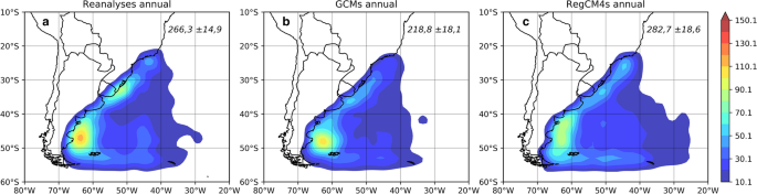
Annual mean of cyclogenesis density (shaded) for the present climate (1979–2005): a reanalyses, b GCMs and c RegCM4 ensembles. The density unit is cyclone per area (km2) × 106 per year. In the right corner of the figures is also shown the annual mean and standard deviation
Figure 3 presents the cyclogenesis (grey lines) and trajectory (shaded) densities from cyclones beginning in each main cyclogenetic region (RG1, RG2 and RG3; see their locations in Fig. 1). For RG1, GCMs and RegCM4s are able to capture the main features of genesis and preferred trajectory of cyclones present in reanalyses (Fig. 3a–c), however, while the GCMs ensemble presents a considerable underestimation of the annual frequency of cyclogenesis (26.6 ± 4.6), RegCM4s (34.4 ± 6.6) is closer to the reanalyses (33.0 ± 6.0). The interannual variability of cyclones in RG1 is also better reproduced by RegCM4s than GCMs as indicated by similar standard deviations of RegCM4s and reanalyses (also shown in Fig. 11). In reanalyses, cyclone trajectories are concentrated near RG1 during most of their lifetime (Fig. 3a). This is correctly represented by the GCMs and RegCM4s (Fig. 3b, c). The concentration of trajectories indicates the quasi-stationary characteristic of most cyclones developing in RG1, also found by Gozzo et al. (2014), while the others have preferential displacement to the southeast.
Fig. 3 
Annual mean of cyclones trajectory density (shaded) and cyclogenesis density (grey lines; intervals of 3.1, 18.1, 30.1, and 70.1) for RG1 (a, b, c—top), RG2 (d, e, f—middle) and RG3 (g, h, i—bottom) hot-spots for: a, d, g reanalyses; b, e, h GCMs; and c, f, i RegCM4s. The density unit is cyclone per area (km2) × 106 per year. The period is the present climate (1979–2005). The right corner of the figures shows the annual mean and standard deviation
The RG2 cyclogenesis hot-spot is located near the border of Uruguay and southern Brazil (Fig. 3d, e, f). In reanalyses, around 37.8 ± 5.7 cyclogeneses per year occur in RG2, with more trajectory density over the region and gradually decreasing to the southeast (Fig. 3d). For RG2, the annual number of cyclogeneses is underestimated by GCMs (34.6 ± 5.4) and overestimated by RegCM4s (40.1 ± 6.2). In terms of trajectories, both ensembles have similar patterns as in reanalyses, but both underestimate (overestimate) the density in the region of maximum near the coast of Uruguay (between 30° and 20°W).
The cyclogenetic region RG3 (Fig. 3g) has the highest number of geneses per year (62.3 ± 7.4) over the eastern coast of South America, which is in agreement with previous studies (Reboita et al. 2010; Krüger et al. 2012; Gramcianinov et al. 2019; Crespo et al. 2020). Despite the similar trajectory density between the three ensembles, GCMs and RegCM4s underestimate the number of cyclogeneses per year (56.3 ± 7.3 and 56.1 ± 7.6, respectively) compared to reanalyses (62.3 ± 7.4). However, having similar standard deviations, the ensembles realistically capture the interannual variability present in reanalyses. In addition, the maximum cyclogenesis and trajectory densities are slightly displaced to the west compared to reanalyses (Fig. 3g–i). In RG3, frequencies and trajectories of cyclones are similar in both simulation ensembles, which can be explained by the greater proximity of the boundary of the RegCM4s domain, resulting in greater influence from GCMs in the regional downscaling.
For a more detailed evaluation, the annual cycles of cyclogenesis frequency in the three main hot-spots and for the SAD are provided in Fig. 4. For RG1 (Fig. 4a), reanalyses present an irregular annual cycle characterized by higher (lower) frequency of cyclones in December-January (March). For most of the months, the simulated frequency of cyclones in RegCM4s is closer to reanalyses than that of GCMs, which is synthetized by a higher correlation coefficient and a lower mean square root error (RMSE). In RG1, the higher frequency of cyclones in the austral summer is more associated with thermodynamics than dynamic forcing mechanisms (Reboita et al. 2010, 2012). Between summer and autumn, the Brazilian current is warmer than in the other seasons and transports warm water poleward (Reboita 2008), which may contribute to the intense transfer of latent and sensible heat to the adjacent air. Moreover, RG1 is a region where the moisture flux transported by the low-level jet and the winds of the South Atlantic Subtropical Anticyclone converge (Gozzo et al. 2014, 2017), initiating a cyclonic circulation. In addition to these thermodynamic processes, the semi-stationary wave at mid-upper levels through the effect of the Andes topography and/or transient waves can disturb the surface, also contributing to cyclogenesis in RG1 (Reboita 2008; Reboita et al. 2012, 2019).
Fig. 4 
Annual cycle of the frequency (lines) and standard deviation (shaded) of cyclogenesis in the present climate (1979–2005) for: a RG1, b RG2, c RG3 and d South Atlantic domains. The correlations and RMSEs between reanalyses and simulations for the annual cycle are indicated in each panel
GCMs and RegCM4s are able to simulate the observed phase and amplitude (high correlations and small RMSEs) of the annual cycle of cyclogenesis frequency in RG2 (Fig. 4b), except by underestimation in the peak months (July–August). In RegCM4, this deficiency was associated with the simulation of mid-level troughs with lower amplitude than in reanalyses (Reboita et al. 2010). A transient trough in the middle-upper troposphere moving from the South Pacific to the South Atlantic is the main forcing for cyclogenesis in RG2 (Reboita et al. 2012).
For RG3, both ensembles simulate most of the features of the annual cycle of cyclogenesis in agreement with reanalyses, except in October (Fig. 4c). This is reflected in a decrease in the correlations between simulations and reanalyses. The weak amplitude (from 5 to 6 events per month in reanalyses) of the annual cycle would be explained by the driver mechanisms occurring during the year in RG3. Cyclogenesis in this region results mainly from the regeneration of systems moving from the west to the east after crossing the Andes and baroclinic instability (Gan and Rao 1991; Hoskins and Hodges 2005; Reboita et al. 2012).
For the SAD, the observed phase and amplitude of cyclogenesis is better reproduced by RegCM4s than GCMs, as indicated by smaller RMSE and similar correlations. The use of an ensemble to obtain RegCM4s results in small biases in the phase and amplitude of the cyclogenesis annual cycle over the SAD and represents a clear improvement compared with previous RegCM3/CMIP3 (Krüger et al. 2012) and only one CREMA member (Reboita et al. 2018).
Histograms of central relative vorticity at cyclogenesis time in each hot-spot are depicted in Fig. 5. Overall, the RegCM4 ensemble improves the GCMs cyclogenesis intensities in both RG1 and RG2 (Fig. 5a, b). There is greater agreement between RegCM4s and reanalyses for both frequencies of weaker and stronger cyclogenesis. For RG3, GCMs are closer to reanalyses, while RegCM4s underestimate the frequency of weaker cyclogenesis (cyclonic vorticity up to − 3 × 10⁻⁵ s−1) and overestimate the stronger ones (Fig. 5c). For the whole SAD both ensembles show a similar frequency of cyclogenesis weaker than − 4 × 10⁻⁵ s−1 as a reflection of each hot-spot region (Fig. 5d). An important point is the better performance of RegCM4s to simulate very intense cyclogenesis, presenting frequencies closer to the reanalysis than GCMs for events up to − 5 × 10⁻⁵ s−1 (Fig. 5d). This kind of cyclogenesis was greatly underestimated in the previous regional downscaling of RegCM3 nested in CMIP3 (Krüger et al. 2012) and the NCEP reanalysis (in the RG2; Reboita et al. 2010).
Fig. 5 
Annual frequency of the relative vorticity (× 10–5 s−1) at cyclogenesis in the present climate (1979–2005) for: a RG1, b RG2, c RG3 and d South Atlantic domains
-
b.
Winds associated with intense cyclones
It is well known that extratropical cyclones are associated with intense near surface winds and upper-level jet streams (Browning 2004; Reboita et al. 2012; Dowdy et al. 2019; Domingues et al. 2019). In this section, we evaluate wind features associated with initially intense cyclones in the three main cyclogenetic hot-spots.
Table 2 presents the thresholds of the 25th percentile of the initial relative vorticity used to characterize intense cyclogenesis in each hot-spot. These thresholds are obtained from the historical period and used to identify intense events in both historical and future periods. As already indicated by the frequency distribution in Fig. 4, the RegCM4s thresholds are closer to reanalyses than GCMs in RG1 and RG2, while the opposite occurs in RG3. Furthermore, comparing the three regions, the stronger cyclogeneses in reanalyses and GCMs occur in RG2, while in RegCM4s are in RG3.
For the present climate, in Fig. 6 we present the composites of the wind at 1000 hPa for stronger cyclogenesis in the three hot-spots selected using the thresholds in Table 2. Figure 6 also highlights the boxes delimiting the area of stronger winds near the coast used to calculate the time series of the mean wind speed discussed in Sect. 3.3. Both simulations reproduce the core of maximum northeasterly winds associated with intense cyclogenesis in RG1 in a similar location compared to the reanalyses (Fig. 6a–c), to the northeast of RG1. Other aspects observed in reanalyses, which are also captured by the ensembles, are the intense easterly winds in the northern sector of the South Atlantic subtropical high and an elongating band of southerly/southeasterly winds from southern Brazil toward northeastern Argentina.
Fig. 6 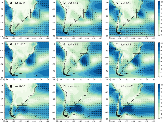
Present climate (1979–2005) composites of the mean wind (arrows and intensity in shaded, m s−1) at 1000 hPa associated with intense cyclones in RG1 (a, b, c—top), RG2 (d, e, f—middle) and RG3 (g, h, i—bottom) hot-spots for: a, d, g reanalyses; b, e, h GCMs; and c, f, i RegCM4s. The rectangles indicate the areas used to calculate the mean wind speed; the values on top of each panel indicates the mean wind and standard deviation inside the respective rectangle
Reanalyses show the maximum northeasterly/northerly winds associated with intense cyclogenesis in RG2 located along the coast, from southeast Brazil to Uruguay (Fig. 6d). The location and intensity of the stronger winds are very well reproduced by the simulations; RegCM4s (Fig. 6f) simulate the region of intense winds in greater agreement with reanalyses than GCMs, which represent an important improvement in the wind field representation compared to GCMs (Fig. 6e). According to reanalyses, the intense cyclogeneses are associated with more intense westerly/northwesterly winds in RG3 (Fig. 6g), and their position is well reproduced by both simulations (Fig. 6h, i).
In general, for the three boxes highlighted in Fig. 6, the wind speed at 1000 hPa is slightly overestimated (~ 0.5 to 2.0 m s−1) by the ensembles, as shown by the mean values in each panel in Fig. 6. In RG1 and RG2, RegCM4s simulate the location of the stronger winds associated with intense cyclones in better agreement with reanalyses compared to GCMs. According to these results, RegCM4s add value to the GCMs in the representation of the near surface wind field. Another important feature from reanalyses is the stronger winds occupying the warm sector (northeast sector in the SH) of the incipient cyclone, which is in accordance with previous studies (Bengtsson et al. 2008) and is very well captured by the ensembles.
The composites of wind at 300 hPa for intense cyclogenesis in each hot-spot are shown in Fig. 7. The upper level jet associated with intense cyclogenesis in RG1 is located to the south of the formation region, with genesis occurring in the equatorial entrance of the jet stream (Fig. 7a–c). According to Crespo et al. (2020), the jet stream for all cyclogenesis occurring in RG1 is more likely to be far from (close to) the region in summer (winter). Nevertheless, the mean in Fig. 7 shows the jet stream near RG1, which is related to a stronger influence of the baroclinic instability for the stronger cyclogenesis. The jet pattern occurs in reanalyses and simulations, but reanalyses have a slightly stronger jet streak compared to the ensembles (Fig. 7a–c).
Fig. 7 
Present climate (1979–2005) composites of the mean wind (arrows; magnitude in shaded, m s−1) at 300 hPa associated with intense cyclones in RG1 (a, b, c—top), RG2 (d, e, f—middle) and RG3 (g, h, i—bottom) hot-spots for: a, d, g Reanalysis; b, e, h GCMs; and c, f, i) RegCM4s. The rectangles indicate the cyclogenetic regions
In reanalyses the upper level jet stream (with two maximum speed cores) is over and downstream RG2 for intense cyclogenesis (Fig. 7d). The location and intensity of the maximum upper-level winds is reasonably well simulated by the ensembles (Fig. 7e, f). However, in simulations the jet stream is more elongated than in reanalyses from the South Pacific, crossing the continent and reaching the South Atlantic.
For RG3, the upper-level jet in the ensembles has a similar pattern in the reanalyses and models (Fig. 7h–j), with GCMs showing greater similarities with reanalyses in the vicinity of RG3 than RegCM4s. The position of the upper-level jet streak confirms the strong influence of baroclinic instability on the cyclogenesis in RG3, which develops in the exit sector of the polar jet.
The previous discussion confirms that the ensembles are able to reproduce the main climatological observed cyclogenesis features (density, trajectory, intensity and associated winds) in eastern South America, which brings confidence to the evaluation of their climate change scenarios.


3.2 Spatial trends: near and far future climates
-
a.
Trajectories
The spatial distributions of the trend in cyclone trajectories for all life cycles starting in the three cyclogenetic hot-spots are shown in Fig. 8. The trend is calculated as the difference of the trajectory densities between the future (near/far) and present climates. Hypothesis tests were not included in cyclones density since they occur in different grid points and we end up with many zeros, which may affect the tests. Therefore, the climate change signal needs to be carefully interpreted since cyclones present high variability and the significance tests tend to be very patchy, as discussed by Pezza et al. (2008, 2012).
Fig. 8 
Trends of trajectories density (future “minus” present) for a, b, e, f, i, j near (2020–2050) and c, d, g, h, k, l far (2070–2099) future climates for GCMs and RegCM4s in a, b, c, d RG1, e, f, g, h RG2 and i, j, k, l RG3. The density unit is cyclone per area (km2) × 106 per year
For the near future, both ensembles present a general decrease in the cyclonic activity near southeastern Brazil and the adjacent ocean, which are the main paths from cyclones starting in RG1 (Fig. 8a, b). Some areas of increasing cyclone trajectories surrounding the main negative core are also projected, mainly to the north in RegCM4s (Fig. 8b). This indicates a shift to the north of preferred paths of cyclones starting in RG1 in the near future climate. For cyclones starting in RG1, the far future climate projections indicate a strong decrease in the cyclone trajectories in a large area surrounding RG1, especially in GCMs (Fig. 8c, d).
In RG2, there is a projection of an increase in cyclone activity in a wide area over the South Atlantic adjacent to the coasts of Uruguay and Argentina in the near future climate although there are still some areas of a weak decrease in cyclone pathways (Fig. 8e, f). This pattern is similar in GCMs and RegCM4s for near future projections, and it is consistent with present climate observations discussed by Reboita et al. (2015). On the other hand, by the end of the century, a predominance of a negative trend in trajectory densities for both ensembles, with some spatial differences, is projected (Fig. 8g, h). The GCMs ensemble projects a greater decrease in cyclone pathways over and near RG2 than RegCM4s, and there is a northwest-southeast “line” of increase in the trajectories in GCMs, also simulated by RegCM4s (Fig. 8g, h). This feature would indicate a shift to the south of the main pathways of cyclones starting in RG2.
There is agreement between ensembles regarding the trajectory density trends for cyclones starting in RG3. Both project a great decrease in the cyclone activity over the South Atlantic, around 45°–50°S, in the near future (Fig. 8i, j), which will become stronger in the far future (Fig. 8k, l). The trends in Fig. 8 agree with the reported decrease in the cyclone frequency over all South Atlantic and a slight increase near Uruguay (Krüger et al. 2012; Reboita et al. 2018, 2020).
-
b.
Lower and upper-level winds
For each cyclognetic hot-spot, Table 3 synthetizes the mean relative vorticity of only initial intense cyclogeneses (25th percentile). They are expected to slightly intensify in the near and far futures in the three hot-spots according to RegCM4s projections, while in GCMs this occurs only for RG1 and in the near future for RG2 (Table 3). The variability of the relative vorticity, as measured by the standard deviation, will also increase in RegCM4s (Table 3). The projected changes in the circulation associated with intense cyclogenesis in the future climate are evaluated considering the trends (future “minus” present climate composites) of the wind, respectively, at 1000 (Fig. 9) and 300 hPa (Fig. 10).
Table 3 Mean and standard deviation of the initial cyclonic vorticity (× 10−5 s−1) for historical (bold) and near (italic) and far (underline) future periods Fig. 9 
Composites of the difference (future “minus” present) of the wind speed at 1000 hPa associated with intense cyclones for a, b, e, f, i, j near (2020–2050) and c, d, g, h, k, l far (2070–2099) future climates for GCMs and RegCM4s in a–d RG1, e–h RG2 and i–l) RG3. The rectangles indicate the regions of stronger winds associated with each cyclogenetic hot-spot in the present climate
Fig. 10 
Composites of the difference (future “minus” present) of the wind speed at 300 hPa associated with intense cyclones for a, b, e, f, i, j near (2020–2050) and c, d, g, h, k, l far (2070–2099) future climates for GCMs and RegCM4s in a–d RG1, e–h RG2 and i–l RG3. The rectangles indicate each one of cyclogenetic hot-spots
In the near future, for intense cyclogenesis there are no remarkable changes in the circulation and wind intensity near the eastern coast of South America at 1000 hPa, except in RG1 for GCMs (Fig. 9a) and RG2 for RegCM4s (Fig. 9f). The former projects a decrease in the wind speed around 44°S (weakening of the westerly winds), while the latter projects an increase over the ocean near Uruguay (36°S–58°W).
Both GCMs and RegCM4s projections indicate the development of an anticyclonic circulation in the RG1 and RG2 composites, located to the southeast of RG1 (Fig. 9a, b; centered on ~ 44°S–35°W) and RG2 (Fig. 9e, f).The establishment of this anticyclonic circulation contributes to reinforce the westerly winds at mid-latitudes (Fig. 9a, b, e, f) and to explain the decrease in the trajectory density during the near future climate for cyclones starting in RG1 since the basic state becomes more unfavorable for cyclogenesis (Fig. 8a, b).
For RG3, the most important projected change in the low-level winds is the intensification of the westerlies near RG3 and the establishment of a cyclonic circulation to the southeast of the region (Fig. 9i, j). These features are more intense in GCMs than in RegCM4s, followed downstream by an anticyclone, as also identified for RG1 and RG2.
Regarding the far future climate, the projections indicate a general increase in the wind speed at 1000 hPa associated with intense cyclogenesis (Fig. 9c, d). For instance, in RG1 the northeasterly winds can be up to 1.5 m s−1 stronger near the southeastern Brazilian coast (Fig. 9c, d). For intense cyclogenesis in RG2, an increase in the 1000 hPa wind speed (up to 1 m s−1) near the southeastern coast of Brazil is also projected (Fig. 9g, h), i.e., to the north of the strongest winds associated with cyclogenesis in the present climate (Fig. 6d–f). Also for RG2, GCMs and RegCM4s indicate a strengthening of the anomalous anticyclone over the South Atlantic (centered on ~ 53°S–35°W), i.e., to the southeast of that for RG1 (Fig. 9c, d). A similar anticyclonic circulation is also identified for the trends in anomaly fields, i.e., when for each period the cyclone composites are subtracted from the current climatology (figure not shown). Therefore, future changes in cyclones (frequency, trajectories, etc.) help to understand the previously documented anomalous anticyclonic circulation found in the mean fields over the South Atlantic in different climate change scenarios (Rauscher et al. 2011; Krüger et al. 2012; Reboita et al. 2018). Another feature that may explain the stronger 1000 hPa wind speed in the future is the slightly stronger cyclogenesis in RG1 and RG2 in RegCM4s (Table 3).
The region of strong low-level winds associated with intense cyclogenesis in RG3 presents a small decrease in the wind speed over the northwestern part of the box in the GCMs (Fig. 9k). In addition, the ensembles project the intensification of low-level winds in two main regions (Fig. 9k, l): far from RG3, i.e., northeasterly winds will increase (up to 2 m s−1) near the southeastern coast of Brazil (~ 30°S; 45°W), associated with the intensification of an anticyclonic circulation in the southeast of the South Atlantic; and to the south of RG3 as a result of the intensification of an anticyclonic circulation (cyclonic circulation) over the South Pacific (South Atlantic) in GCMs in about ~ 48°–58°S (RegCM4s). Near the southern part of the domain, the increase in the wind intensity would be a response of the more intense horizontal pressure gradients in the future climate as discussed by Reboita et al. (2020).
At upper levels, near future projections indicate an increase in the jet speed near the cyclogenetic regions RG1 and RG2 and a decrease to the south, indicating a weakening (strengthening) in the upper-level polar jet (subtropical jet) associated with intense cyclogenesis (Fig. 10a, b, e, f). For RG3, GCMs (RegCM4s) simulate a decrease (increase) in the jet speed upstream (northward and over) the cyclogenetic region (Fig. 10i, j).
For the far future, there is a strengthening of the upper level jet anomalies for the three regions (Fig. 10c, d, g, h, k, l); while GCMs project stronger anomalies for RG1 than RegCM4s (Fig. 10c, d), in RegCM4s the anomalies for RG2 and RG3 are greater (Fig. 10g, h, k, l) than in GCMs. Both RG1 and RG2 will be influenced in the far future by positive anomalies of the upper level jet speed; RG1, specifically, will be located right under the jet streak entrance (Fig. 10c, d) while RG2 will be located under the polar exit sector of the jet streak (Fig. 10g, h). This suggests that intense cyclogenesis in RG1 and RG2 will occur under stronger upper-level jets in the future. For RG3, however, this signal is not so clear (Fig. 10k, l).
In general, far future projections indicate a shift to the south of the jets, which is identified by (1) the weakening of the polar jet in the latitudinal band of 36°S–50°S and strengthening to the south, which is a pattern consistent with the shift to the south of the climatological baroclinic zone; (2) a strengthening of the subtropical jet, from the South Pacific to the South Atlantic in the latitudinal band of 18°S–36°S, directly affecting RG1 and RG2. This strengthening in the upper-level jet leads to a deepening in the stationary trough over the Andes which generates (a) stronger cyclogenesis, and, especially, the positive trajectory anomalies projected from cyclones starting in RG2; and (b) the formation of a ridge/anticyclone downstream, which lies above the 1000 hPa anticyclonic anomalies (20°S–40°W to 50°S–30°W; Fig. 10), therefore configuring a barotropic response to global warming; and (3) a strengthening of the easterly winds in tropical latitudes northward of 18°S. These patterns have similarities to that found by Reboita et al. (2018) for projections of the winter season winds at upper levels, i.e., irrespective of whether there are cyclogeneses or not.


3.3 Long-term mean trends: cyclogenesis and winds
Another way to evaluate the trends of cyclogenesis in the hot-spots is through the time series of the annual frequency of events (Fig. 11).

Observed (1979–2005) and simulated (1979–2099) time series of the annual mean frequency of cyclogenesis in RG1 (red colors), RG2 (blue colors) and RG3 (green colors). The bold lines indicate the trends
As discussed before in the spatial maps, a higher (lower) number of cyclogeneses in RegCM4s (GCMs) than in reanalyses is observed. Nevertheless, according to Fig. 11, RegCM4s have more ability to simulate the observed frequency of cyclones in RG1 in the present climate, while GCMs show a greater underestimation as already mentioned (Figs. 3, 4). This might be due to the greater ability of RegCM4s to resolve smaller scale cyclonic systems and diabatic processes which are important for most of the cyclogeneses in this region, as proposed by Gozzo et al. (2014).
For RG2, despite the closer proximity between the trend lines of GCMs and reanalyses, on average for the present climate a similar bias in cyclone frequency for both ensembles can be seen (Fig. 11); the overestimation is + 6% in RegCM4s, and the underestimation reaches − 8% in GCMs. Both biases are relatively small since they do not exceed ± 10%. In the present climate, the underestimation of the annual frequency of cyclones is similar for both ensembles in RG3 (Fig. 11).
There is a clear trend toward a decrease in the frequency of cyclones in the present climate for the three cyclogenetic hot-spots in the reanalyses (Fig. 11). Among the three regions, reanalyses present a less steep decrease for RG2 and RG3 and a stronger negative trend in RG1.The simulations are able to reproduce the reanalysis trends in RG2 and RG3 but not in RG1. It is important to highlight that for the 27 years of the present climate the negative trends in Fig. 11 are not statistically significant at the 95% level (p-value > 0.05) according to the Mann–Kendall statistical test (Kendall 1975; Mann 2008).
For the future climate, GCMs and RegCM4s followed the same negative trend lines until the end of the twentieth century in RG1 and RG2, but they diverge after ~ 2020–2030 in RG3 when GCMs present a steeper negative trend than RegCM4s (Fig. 11). For the whole period (1979–2099), the Mann–Kendall test indicates that the projected negative trends are statistically significant (p-value < 0.05).
For the three cyclogenetic hot-spots, reanalyses show a strong interannual variability in the frequency of cyclones, which is better captured by RegCM4s than GCMs in the present climate (Fig. 11). This feature is a very important added value of the dynamic downscaling, giving confidence to the regional projections that continue to also indicate greater interannual variability in the future climate. Another very useful piece of information is the presence of low frequency (decadal to multidecadal) variability of the cyclone frequency superimposed on the general decrease; i.e., even projecting a general negative trend, cyclones will be more/less frequent in some decades than in others (Fig. 11).
The projection of decrease in the frequency of cyclones in each cyclogenetic hot-spot contributes to a general negative trend for all cyclones over the SAD (Fig. 12). In this case, a clear improvement of the dynamical downscaling in reproducing reanalyses for both frequency and trend in the present climate is also noted.

Observed (1979–2005) and simulated (1979–2099) time series of the annual mean frequency of cyclogenesis in all South Atlantic domain. The bold lines indicate the trends
In order to synthetize the trends of winds at 1000 hPa associated with intense cyclogenesis, Fig. 13 presents the annual average of the stronger winds in the present climate for each region (delimited boxes highlighted in Figs. 6, 9). For the present climate, GCMs and RegCM4s overestimate (by ~ 2 m s−1) reanalysis wind speed associated with intense cyclones in RG3. However, for RG1 and RG2 the biases (of ~ 1 m s−1) are very small and of the same order as the underestimation of local observations of near surface wind speeds by reanalyses (Cardoso 2019).

Observed (1979–2005) and simulated (1979–2099) time series of the annual averaged wind speed at 1000 hPa associated with intense cyclones (and linear trend lines) in RG1 (red colors), RG2 (blue colors) and RG3 (green colors). These averages were calculated in the region of maximum wind speed associated with intense cyclones in the present climate (boxes in Figs. 6, 9)
Reanalyses indicate a positive trend in the wind speed at 1000 hPa associated with intense cyclones starting in RG1, which is not captured by the ensembles (Fig. 13). Since in reanalyses (and RegCM4s) the frequency of cyclones is decreasing (both total—Fig. 11—and intense cyclones—figure not shown), each event is associated with stronger winds. On the other hand, GCMs have a different behavior since their projections indicate an increase in stronger cyclogenesis (figure not shown). For the future climate, the intensity of such winds will be similar to the present climate according to the ensembles (Fig. 13). However, since the frequency is decreasing in RegCM4s, each cyclone will have stronger winds, but the opposite behavior is projected by GCMs.
There is also a positive trend in the wind speed for stronger cyclones starting in RG2 in reanalyses, which is very well captured by the ensembles (Fig. 13). In this region, both ensembles project the same trend in the future, as well as the negative trend of the intense events. For RG3, RegCM4s capture both the weak positive trend of the wind speed and the negative trend of these events (figure not shown) as in reanalyses while GCMs do not present any trend in the wind speed (Fig. 13). As for the cyclone frequency, only the long term (1979–2099) trends of wind speed at 1000 hPa (Fig. 13) are statistically significant (p-value < 0.05) according to Mann–Kendall test.
4 Summary and concluding remarks
In this study, we use multi-model ensembles to understand regional features of future climate trends of cyclones from the three main cyclogenetic hot-spots (RG1, RG2 and RG3) and associated winds in eastern South America. For this, we consider three mini-ensembles, composed by four RegCM4 and three GCMs climate projections, and two reanalyses. Focusing on cyclones starting in these hot-spots, we analyze the: (1) ability of the ensembles to reproduce cyclogenesis features and winds associated with intense cases in the present climate (1979–2005), using reanalysis as reference; and (2) projections of cyclones and associated winds for near (2020–50) and far (2070–99) future RCP8.5.
For the present climate, RegCM4s and GCMs simulate the main characteristics of cyclone genesis and propagation, leading to the conclusion that models could present consistent climate change scenarios. On a regional scale, the annual frequency of cyclogenesis in RG1 is best represented by RegCM4s; in RG2 it is overestimated/underestimated in the same way, and in RG3 it is overestimated by both ensembles. For each cyclogenetic hot-spot, through cyclogenesis and trajectory densities, it is confirmed that RegCM4s and GCMs simulate the locations and the annual cycles similar to reanalyses. An important added value is the greater ability of RegCM4s to capture the reanalysis features (annual number of events, phase and amplitude of the annual cycle and intensity) of cyclogeneses starting in the hot-spots that are away from its boundary domain, i.e., in RG1 and RG2, which does not occur in RG3. This last region is closer to the RegCM4s lateral boundary, where GCMs exert a stronger forcing on the simulation and regional downscaling, better reflecting the large scale characteristics. For the hot-spots away from the boundary, the regional model fine resolution and physical parameterization have a great degree of freedom to solve diabatic and local circulation processes conducting to cyclogenesis, especially in RG1 and RG2, where diabatic heating associated with moist convection and/or air-sea interaction are important for cyclone development (da Rocha et al. 2010; Reboita et al. 2012; Piva et al. 2011; Gozzo and da Rocha 2013; Gozzo et al. 2014). In addition, compared to previous analyses of only one member (Reboita et al. 2018; Krüger et al. 2012), the use of an ensemble of simulations also attains more realistic reproduction of cyclone climatology in the region. Therefore, these results point out the advantages of using an ensemble of regional downscaling to analyze cyclones over the eastern coast of South America.
For the three hot-spots, reanalyses and ensembles show stronger low-level winds associated with intense cyclogenesis occuring preferably in its northeastern sector (warm cyclone sector). However, there is greater agreement between RegCM4s and reanalyses regarding the magnitude and location of these stronger winds for RG1 and RG2, which represents an important RegCM4 added value to the GCMs. As expected, both ensembles realistically represent the intensity and location of the upper-level jet, with small differences compared to reanalysis and which do not compromise the evaluation in future climate projections.
While in the far future scenario both ensembles project an intense decrease in cyclones, for the near future projections the signal is weaker and not homogeneous with specific regional differences: (1) RG3 presents a trend toward a decrease in cyclogenetic activity; (2) RG1 indicates a general decrease in the cyclonic activity near the southeastern Brazilian coast and a shift to the north of their preferred paths; (3) RG2 shows an increase in the cyclone activity in a wide area over the ocean near the coasts of Uruguay and Argentina. This last trend agrees with previous near future projection studies (Krüger et al. 2012; Reboita et al. 2018, 2020).
In terms of the mean circulation associated with intense cyclogenesis (the 25th lower percentile of minimum relative vorticity), at upper levels the far future projections indicate: a shift to the south of the polar jet, which is a pattern consistent with the displacement to the south of the climatological baroclinic zone; a strengthening of the subtropical jet, from the South Pacific to the South Atlantic, which generates (1) stronger cyclogenesis, and, especially, the positive trajectory anomalies projected for cyclones starting in RG2; and (b) the formation of a ridge/anticyclone downstream. This ridge lies above the low-level anticyclonic anomalies and therefore results in a barotropic response to global warming.
A common and important projected change for the far future is the intensification of the low-level winds, associated with intense cyclogenesis, near the coast of southeastern Brazil. These winds will become stronger in the eastern/northeastern sectors (warm sector in the SH) of cyclogenesis. This mainly occurs as a consequence of the intensification of the northwestern branch of anomalous anticyclonic circulation over the southeastern South Atlantic, which is on average centered on ~ 35°W, but more to the north (~ 40°S) for RG1 and to the south (~ 46°S) for RG2 and RG3 intense cyclogenesis.
Finally, for the present climate, there is a clear negative trend of the cyclogenesis frequency for each hot-spot, especially in RG1, where reanalyses present a stronger negative trend, which is underestimated by the ensembles. For the three hot-spots, the ensembles project negative trends of the frequency of intense cyclones to persist into the far future together with an increase in the associated low-level wind speeds. Therefore, the long term projections indicate that each intense cyclone will be associated with stronger low-level wind speed near the South America eastern coast in the far future climate.
This study highlights the importance of monitoring cyclogenesis near the southern/southeastern coast of Brazil using climate models and how ensembles, especially those of regional climate models, are able to represent important observed features related to all (and intense) cyclogeneses over the South America eastern coast. Understanding how the low-level winds associated with intense cyclones will change in the future climate is essential for future planning and mitigation strategies in order to avoid damage to the population and economy. A further analysis considering specific types of cyclones, such as explosive (also called bombs) and subtropical cyclones in the future climate projections would be valuable since these systems cause considerable damage along the South American coast.
References
Allen JT, Pezza AB, Black MT (2010) Explosive cyclogenesis: a global climatology comparing multiple reanalyses. J Clim 23:6468–6484
Banerjee A, Fyfe JC, Polvani LM, Waugh D, Chang KL (2020) A pause in Southern Hemisphere circulation trends due to the Montreal Protocol. Nature 579:544–548
Bengtsson LO, Hodges KI (2005) Storm tracks and climate change. J Clim 19:3518–3543
Bengtsson LO, Hodges KI, Keenlyside N (2008) Will extratropical storms intensity in a warmer climate? J Clim 22:2276–2301. https://doi.org/10.1175/2008JCLI2678.1
Bentley AM, Bosart LF, Keyser D (2019) A climatology of extratropical cyclones leading to extreme weather events over central and eastern North America. Mon Weather Rev 147:1471–1490
Blender R, Fraedrich K, Lunkeit F (1997) Identification of cyclone-track regimes in the North Atlantic. Q J R Meteorol Soc 123:727–741
Brâncuş M, Schultz DM, Antonescu B, Dearden C, Ştefan S (2019) Origin of strong winds in an explosive mediterranean extratropical cyclone. Mon Weather Rev 147:3649–3671
Browning KA (2004) The sting at the end of the tail: damaging winds associated with extratropical cyclones. Q J R Meteorol Soc 130:375–399. https://doi.org/10.1256/qj.02.143
Cardoso AA (2019) Ciclones subtropicais e ventos em superfície no sudoeste do Oceano Atlântico Sul: climatologia e extremos. Master thesis, Universidade de São Paulo
Catto JL, Ackerley D, Booth JF et al (2019) The future of midlatitude cyclones. Curr Clim Change Rep 5:407–420
Cecilio RO, Dillenburg SR (2019) An ocean wind-wave climatology for the Southern Brazilian Shelf. Part II: variability in space and time. Dyn Atmos Oceans 88:101103
Champion AJ, Hodges KI, Bengtsson LO, Keenlyside NS, Esch M (2011) Impact of increasing resolution and a warmer climate on extreme weather from Northern Hemisphere extratropical cyclones. Tellus A 63:893–906
Chang EKM (2017) Projected significant increase in the number of extreme extratropical cyclones in the Southern Hemisphere. J Clim 30:4915–4935
Chang EKM (2018) Projected change in Northern Hemisphere winter cyclones with associated extreme winds. J Clim 31:6527–6542
Crespo NM, da Rocha RP, Sprenger M, Wernli H (2020) A potential vorticity perspective on cyclogenesis over centre-eastern South America. Int J Climatol 2020:1–16. https://doi.org/10.1002/joc.6644
da Rocha RP, Caetano E (2010) The role of convective parameterization in the simulation of a cyclone over the South Atlantic. Atmósfera 23:1–23
da Rocha RP, Sugahara S, da Silveira RB (2004) Sea waves generated by extratropical cyclones in the South Atlantic Ocean: hindcast and validation against altimeter data. Wea Forecasting 19:398–410. https://doi.org/10.1175/1520-0434(2004)019%3c0398:SWGBEC%3e2.0.CO;2
da Rocha RP, Reboita MS, Dutra LMM, Llopart MP, Coppola E (2014) Interannual variability associated with ENSO: present and future climate projections of RegCM4 for South America-CORDEX domain. Clim Change 125:95–109
Dee DP, Uppala SM, Simmons AJ et al (2011) The ERA-Interim reanalysis: configuration and performance of the data assimilation system. Q J R Meteorol Soc 137:553–597
Dickinson RE, Henderson-Sellers A, Kennedy PJ (1993) Biosphere-atmosphere Transfer Scheme (BATS) Version 1e as Coupled to the NCAR Community Climate Model (No. NCAR/TN-387+STR). University Corporation for Atmospheric Research. https://doi.org/10.5065/D67W6959
Domingues R, Kuwano-Yoshida A, Chardon-Maldonado P et al (2019) Ocean observations in support of studies and forecasts of tropical and extratropical cyclones. Front Mar Sci. https://doi.org/10.3389/fmars.2019.00446
Dowdy AJ, Pepler A, Di Luca A et al (2019) Review of Australian east coast low pressure systems and associated extremes. Clim Dyn 53:4887–4910. https://doi.org/10.1007/s00382-019-04836-8
Dunne JP, John JG, Adcroft AJ et al (2012) GFDL’s ESM2 global coupled climate–carbon earth system models. Part I: physical formulation and baseline simulation characteristics. J Clim 25:6646–6665
Emanuel KA, Zivkovic-Rothman M (1999) Development and evaluation of a convection scheme for use in climate models. J Atmos Sci 56:1766–1782
Feng X, Huang B, Tintera G, Chen B (2019) An examination of the Northern Hemisphere mid-latitude storm track interannual variability simulated by climate models—sensitivity to model resolution and coupling. Clim Dyn 52:4247–4268
Flaounas E, Kotroni V, Lagouvardos K, Flaounas I (2014) CycloTRACK (v1. 0)–tracking winter extratropical cyclones based on relative vorticity: sensitivity to data filtering and other relevant parameters. Geosci Model Dev 7:1841–1853
Fyfe JC (2003) Extratropical Southern Hemisphere cyclones: harbingers of climate change? J Clim 16:2802–2805
Gan MA, Rao VB (1991) Surface cyclogenesis over South America. Mon Weather Rev 119:1293–1302
Giorgetta MA, Jungclaus J, Reicket CH et al (2013) Climate and carbon cycle changes from 1850 to 2100 in MPI-ESM simulations for the Coupled Model Intercomparison Project phase 5. J Adv Model Earth Sy 5:572–597. https://doi.org/10.1002/jame.20038
Giorgi F (2014) Introduction to the special issue: the phase I CORDEX RegCM4 hyper-matrix (CREMA) experiment. Clim Change 125:1–5. https://doi.org/10.1007/s10584-014-1166-4
Giorgi F (2019) Thirty years of regional climate modeling: where are we and where are we going next? JGR Atmos 124:5696–5723. https://doi.org/10.1029/2018JD030094
Giorgi F, Coppola E, Solmon F et al (2012) RegCM4: model description and preliminary tests over multiple CORDEX domains. Clim Res 52:7–29. https://doi.org/10.3354/cr01018
Gozzo LF, da Rocha RP (2013) Air–sea interaction processes influencing the development of a Shapiro-Keyser type cyclone over the subtropical South Atlantic Ocean. Pure Appl Geophys 170:917–934. https://doi.org/10.1007/s00024-012-0584-3
Gozzo LF, da Rocha RP, Reboita MS, Sugahara S (2014) Subtropical cyclones over the southwestern South Atlantic: climatological aspects and case study. J Clim 27:8543–8562
Gozzo LF, da Rocha RP, Gimeno L, Drumond A (2017) Climatology and numerical case study of moisture sources associated with subtropical cyclogenesis over the southwestern Atlantic Ocean. J Geophys Res Atmos 122:5636–5653
Gramcianinov CB, Hodges KI, Camargo R (2019) The properties and genesis environments of South Atlantic cyclones. Clim Dyn 53:4115–4140
Grell GA (1993) Prognostic evaluation of assumptions used by cumulus parameterizations. Mon Weather Rev 121:764–787
Grise KM, Son SW, Correa GJ, Polvani LM (2014) The response of extratropical cyclones in the Southern Hemisphere to stratospheric ozone depletion in the 20th century. Atmos Sci Lett 15:29–36
Hanley J, Caballero R (2012) Objective identification and tracking of multicentre cyclones in the ERA-Interim reanalysis dataset. Q J R Meteorol Soc 138:612–625. https://doi.org/10.1002/qj.948
Hawcroft M, Walsh E, Hodges K, Zappa G (2018) Significantly increased extreme precipitation expected in Europe and North America from extratropical cyclones. Environ Res Lett. https://doi.org/10.1088/1748-9326/aaed59
Holtslag AAM, de Bruijn EIF, Pan HL (1990) A high resolution air mass transformation model for short-range weather and fore- casting. Mon Weather Rev 118:1561–1575
Hoskins BJ, Hodges KI (2005) A new perspective on southern hemisphere storm tracks. J Clim 18:4108–4129
Kendall MG (1975) Rank correlation methods, 4th edn. Charles Griffin, London
Kiehl JT, Hack JJ, Bonan GB, Boville BA, Briegleb BP, Williamson DL, Rasch PJ (1996) Description of the NCAR Community Climate Model (CCM3) (No. NCAR/TN-420+STR). University Corporation for Atmospheric Research. https://doi.org/10.5065/D6FF3Q99
Knox JA, Frye JD, Durkee JD, Fuhrmann CM (2011) Non-convective high winds associated with extratropical cyclones. Geogr Compass 5:63–89
Knutti R, Furrer R, Tebaldi C, Cermak J, Meehl GA (2010) Challenges in combining projections from multiple climate models. J Clim 23:2739–2758
Krüger LF, da Rocha RP, Reboita MS, Ambrizzi T (2012) RegCM3 nested in HadAM3 scenarios A2 and B2: projected changes in extratropical cyclogenesis, temperature and precipitation over the South Atlantic Ocean. Clim Change 113:599–621
Leckebusch GC, Ulbrich U (2004) On the relationship between cyclones and extreme windstorm events over Europe under climate change. Glob Planet Change 44:181–193
Llopart M, Coppola E, Giorgi F, da Rocha RP, Cuadra SV (2014) Climate change impact on precipitation for the Amazon and La Plata basins. Clim Change 125:111–125
Machado AA, Calliari LJ (2016) Synoptic systems generators of extreme wind in Southern Brazil: atmospheric conditions and consequences in the coastal zone. J Coast Res 75:1182–1186
Mann ME (2008) Smoothing of climate time series revisited. Geophys Res Lett. https://doi.org/10.1029/2008GL034716
Marciano CG, Lackmann GM, Robinson WA (2015) Changes in U.S. east coast cyclone dynamics with climate change. J Clim 28:468–484. https://doi.org/10.1175/JCLI-D-14-00418.1
Martin GM, Bellouin N, Collins WJ et al (2011) The HadGEM2 family of Met Office Unified Model climate configurations. Geosci Model Dev 4:723–757. https://doi.org/10.5194/gmd-4-723-2011
Martínez-Alvarado O, Gray SL, Hart NC, Clark PA, Hodges KI, Roberts MJ (2018) Increased wind risk from sting-jet windstorms with climate change. Environ Res Lett. https://doi.org/10.1088/1748-9326/aaae3a
Mbengue C, Schneider T (2017) Storm-track shifts under climate change: toward a mechanistic understanding using baroclinic mean available potential energy. J Atmos Sci 74:93–110
McDonald RE (2011) Understanding the impact of climate change on Northern Hemisphere extra-tropical cyclones. Clim Dyn 37:1399–1425
Ming Y, Ramaswamy V, Chen G (2011) A model investigation of aerosol-induced changes in boreal winter extratropical circulation. J Clim 24:6077–6091. https://doi.org/10.1175/2011JCLI4111.1
Mizuta R (2012) Intensification of extratropical cyclones associated with the polar jet change in the CMIP5 global warming projections. Geophys Res Lett. https://doi.org/10.1029/2012GL053032
Muis S, Verlaan M, Winsemius HC, Aerts JC, Ward PJ (2016) A global reanalysis of storm surges and extreme sea levels. Nat Commun 7:1–12
Murray RJ, Simmonds I (1991) A numerical scheme for tracking cyclone centers from digital data. Part I: development and operation of the scheme. Aust Meteor Mag 39:155–166
Necco GV (1982) Comportamiento de Vortices Ciclonicos En El Area Sudamerica Durante El FGGE: cyclogenesis. Meteorologica 13:7–19
Neu U et al (2013) IMILAST: a community effort to intercompare extratropical cyclone detection and tracking algorithms. Bull Amer Meteor Soc 94:529–547. https://doi.org/10.1175/BAMS-D-11-00154.1
Pal JS, Small EE, Elthair EA (2000) Simulation of regional-scale water and energy budgets: representation of subgrid cloud and precipitation processes within RegCM. J Geophys Res 105:29579–29594
Peixoto JP, Oort AH (1992) Physics of climate. Am Inst of Phys, New York
Pepler AS, Di Luca A, Ji F, Alexander LV, Evans JP, Sherwood SC (2016) Projected changes in east Australian midlatitude cyclones during the 21st century. Geophys Res Lett 43:334–340. https://doi.org/10.1002/2015GL067267
Pezza AB, Ambrizzi T (2003) Variability of Southern Hemisphere cyclone and anticyclone behavior: further analysis. J Clim 16:1075–1083
Pezza AB, Durrant T, Simmonds I, Smith I (2008) Southern hemisphere synoptic behavior in extreme phases of SAM, ENSO, sea ice extent, and southern Australia rainfall. J Clim 21:5566–5584
Pezza AB, Rashid HA, Simmonds I (2012) Climate links and recent extremes in antarctic sea ice, high-latitude cyclones, Southern Annular Mode and ENSO. Clim Dyn 38:57–73
Pfahl S, Wernli H (2012) Quantifying the relevance of cyclones for precipitation extremes. J Clim 25:6770–6780
Pfahl S, O’Gorman PA, Singh MS (2015) Extratropical cyclones in idealized simulations of changed climates. J Clim 28:9373–9392
Piva ED, Gan MA, Moscati MCL (2011) The role of latent and sensible heat fluxes in an explosive cyclogenesis over the south American east coast. J Meteor Soc Japan 89:637–663
Pryor SC, Barthelmie RJ, Clausen NE, Drews M, MacKellar N, Kjellstrom E (2012) Analyses of possible changes in intense and extreme wind speeds over northern Europe under climate change scenarios. Clim Dyn 38:189–208
Rauscher SA, Kucharski F, Enfield DB (2011) The role of regional SST warming variations in the drying of meso-america in future climate projections. J Clim 24:2003–2016
Reboita MS (2008) Ciclones extratropicais sobre o Atlântico Sul: Simulação climática e experimentos de sensibilidade. Dissertation, Universidade de São Paulo
Reboita MS, da Rocha RP, Ambrizzi T, Sugahara S (2010) South Atlantic ocean cyclogenesis climatology simulated by regional climate model (RegCM3). Clim Dyn 35:1331–1347. https://doi.org/10.1007/s00382-009-0668-7
Reboita MS, da Rocha RP, Ambrizzi T (2012) Dynamic and climatological features of cyclonic developments over southwestern South Atlantic Ocean. In: B. Veress, J. Szigethy (Eds.) Horizons in Earth Science Research, 6th edn. Nova Science Publishers, Inc., pp 135–160
Reboita MS, da Rocha RP, Ambrizzi T, Gouveia CD (2015) Trend and teleconnection patterns in the climatology of extratropical cyclones over the Southern Hemisphere. Clim Dyn 45:1929–1944
Reboita MS, da Rocha RP, de Souza MR, Llopart M (2018) Extratropical cyclones over the southwestern South Atlantic Ocean: HadGEM2-ES and RegCM4 projections. Int J Climatol 38:2866–2879
Reboita MS, da Rocha RP, Oliveira DM (2019) Key features and adverse weather of the named subtropical cyclones over the Southwestern South Atlantic Ocean. Atmosphere 10:6
Reboita MS, Reale M, da Rocha RP et al (2020) Future changes in the wintertime cyclonic activity over the CORDEX-CORE southern hemisphere domains in a multi-model approach. Clim Dyn. https://doi.org/10.1007/s00382-020-05317-z
Riahi K, Rao S, Krey V et al (2011) RCP 8.5—a scenario of comparatively high greenhouse gas emissions. Clim Change. https://doi.org/10.1007/s10584-011-0149-y
Ribeiro RB, Sampaio AFP, Ruiz MS, Leitão JC, Leitão PC (2019) First approach of a storm surge early warning system for Santos region. In: Climate Change in Santos Brazil: Projections, Impacts and Adaptation Options. https://doi.org/10.1007/978-3-319-96535-2_7
Saha S, Moorthi S, Pan HL et al (2010) The NCEP climate forecast system reanalysis. Bull Am Meteorol Soc 91:1015–1058. https://doi.org/10.1175/2010BAMS3001.1
Satyamurty P, Santos RP, Lems MAM (1980) On the stationary trough generated by the Andes. Mon Weather Rev 108:510–520
Seluchi M (1995) Diagnóstic Y Prognóstico de Situaciones Sinópticas Conducentes a Ciclogénesis sobre el Este de Sudamérica. Geofísica Int 34:171–186
Shaw TA, Baldwin M, Barnes EA et al (2016) Storm track processes and the opposing influences of climate change. Nat Geosci 9:656–664
Silva GAM, Drumond A, Ambrizzi T (2011) The impact of El Niño on South American summer climate during different phases of the Pacific Decadal Oscillation. Theor Appl Climatol 106:307–319. https://doi.org/10.1007/s00704-011-0427-7
Simmonds I, Keay K (2000) Variability of Southern Hemisphere extratropical cyclone behavior, 1958–97. J Clim 13:550–561
Sinclair MR (1994) An objective cyclone climatology for the Southern Hemisphere. Mon Weather Rev 122:2239–2256
Sinclair MR (1995) A climatology of cyclogenesis for the southern hemisphere. Mon Weather Rev 123:1601–1619
Sinclair MR (1996) Reply. Mon Weather Rev 124:2615–2618
Tamarin-Brodsky T, Kaspi Y (2017) Enhanced poleward propagation of storms under climate change. Nat Geosci 10:908–913
Tawfik AB, Steiner AL (2011) The role of soil ice in land-atmosphere coupling over the United States: a soil moisture– precipitation winter feedback mechanism. J Geophys Res. https://doi.org/10.1029/2010JD014333
Taylor KE, Stouffer RJ, Meehl GA (2012) An overview of CMIP5 and the experiment design. Bull Amer Meteor Soc 93:485–498
Tierney G, Posselt DJ, Booth JF (2018) An examination of extratropical cyclone response to changes in baroclinicity and temperature in an idealized environment. Clim Dyn 51:3829–3846
Trenberth KE (1991) Storm tracks in the Southern Hemisphere. J Atmos Sci 48:2159–2178
Utsumi N, Kim H, Kanae S, Oki T (2017) Relative contributions of weather systems to mean and extreme global precipitation. J Geophys Res 122:152–167. https://doi.org/10.1002/2016JD025222
Vera C, Vigliarolo PK, Berbery EH (2002) Cold season synoptic-scale waves over subtropical South America. Mon Weather Rev 130:684–699
Wang XL, Feng Y, Compo GP, Swail VR, Zwiers FW, Allan RJ, Sardeshmukh PD (2013) Trends and low frequency variability of extra-tropical cyclone activity in the ensemble of twentieth century reanalysis. Clim Dyn 40:2775–2800
Wang XL, Feng Y, Chan R, Isaac V (2016) Inter-comparison of extra-tropical cyclone activity in nine reanalysis datasets. Atmos Res 181:133–153
Watterson IG (2006) The intensity of precipitation during extratropical cyclones in global warming simulations: a link of cyclone intensity? Tellus 58:82–97
Willison J, Robinson WA, Lackmann GM (2013) The importance of resolving mesoscale latent heating in the North Atlantic storm track. J Atmos Sci 70:2234–2250
Wu Y, Ting M, Seager R, Huang HP, Cane MA (2011) Changes in storm tracks and energy transports in a warmer climate simulated by the GFDL CM2.1 model. Clim Dyn 37:53–72
Zappa G (2019) Regional climate impacts of future changes in the mid-latitude atmospheric circulation: a storyline view. Curr Clim Change Rep 5:358–371
Zappa G, Shaffrey LC, Hodges KI, Sansom PG, Stephenson DB (2013) A multimodel assessment of future projections of North Atlantic and European extratropical cyclones in the CMIP5 climate models. J Clim 26:5846–5862
Acknowledgements
The authors acknowledge Coordenação de Aperfeiçoamento de Pessoal de Nível Superior (CAPES) Finance Code 001, Conselho Nacional de Desenvolvimento Científico e Tecnológico (CNPq Grants #430314/2018-3, #304949/2018-3, #420262/2018-0, #305304/2017-8, 141869/2017-8) and PETROBRAS (2017/00671-3) for the financial support, and to the anonymous reviewers for their valuable suggestions to organize and improve the manuscript.
Funding
This study was funded by (a) Coordenação de Aperfeiçoamento de Pessoal de Nível Superior (CAPES); (b) Conselho Nacional de Desenvolvimento Científico e Tecnológico (CNPq); (c) PETROBRAS.
Author information
Authors and Affiliations
Corresponding author
Ethics declarations
Conflict of interest
The authors declare that there are no conflicts of interest.
Additional information
Publisher's Note
Springer Nature remains neutral with regard to jurisdictional claims in published maps and institutional affiliations.
Rights and permissions
About this article

Cite this article
de Jesus, E.M., da Rocha, R.P., Crespo, N.M. et al. Multi-model climate projections of the main cyclogenesis hot-spots and associated winds over the eastern coast of South America. Clim Dyn 56, 537–557 (2021). https://doi.org/10.1007/s00382-020-05490-1
Received:
Accepted:
Published:
Issue Date:
DOI: https://doi.org/10.1007/s00382-020-05490-1