
Abstract
This study reinspects the dominant modes of different types of El Niño from the perspectives of monthly mean and seasonality using a combined technique referred as RC-REOF. Several features have been revealed. (1) The explained variances of eastern Pacific (EP) El Niño and central Pacific (CP) El Niño are comparable, in the ranges of 33–43 and 23–28 %, respectively. (2) This feature is more in line with the frequent occurrence of CP El Niño compared to the result from orthogonal EOF analysis in which El Niño Modoki explains a smaller variance of 11–12 %. (3) Both special patterns of EP El Niño and CP El Niño are of equatorial asymmetry that is often overlooked previously by the traditional Niño indices. Based on the features captured by the two leading RC-REOF modes, the authors propose a new pair of Niño indices referred to as Niño3b and Niño4b that have the following advantages: (1) simple calculation, (2) robust and stable relationship with the EP/CP El Niño modes, (3) more representative for Pacific decadal signals, (4) easier to distinguish ENSO types, and (5) without restriction by orthogonality, and others. The Niño3b and Niño4b indices are potentially useful for both scientific research and real-time monitoring of the two types of El Niño. Besides, an index namely Niño3.4b is also introduced to describe the hybrid ENSO events, with relatively equal covariance to EP El Niño and CP El Niño and with larger covariance at decadal time scale than index Niño3.4.
1 Introduction
As one of the most important factors that affect the world’s climate, El Niño/Southern Oscillation (ENSO) causes large-range atmospheric circulation and weather-climate anomalies via “atmospheric bridge”—teleconnections induced by upper-level divergent perturbation (e.g., Wallace and Gutzler 1981; Sardeshmukh and Hoskins 1988). Any strong changes in ENSO would result in profound climatic, ecological, agricultural and socioeconomic consequences (e.g., Latif and Keenlyside 2009; Cai et al. 2014, 2015b). In the past three decades, a new-fashioned central Pacific (CP) El Niño (e.g., Graf 1986; Yu and Kao 2007; Kao and Yu 2009; Yu and Kim 2010; Graf and Zanchettin 2012), also named “western-type El Niño” (Fu and Fletcher 1985), “Dateline El Niño” (Larkin and Harrison 2005), “El Niño Modoki” (Ashok et al. 2007), “warm-pool El Niño” (Kug et al. 2009), and “CP warming” (Kim et al. 2009), occurs more and more intensely and frequently in the context of global warming (e.g., Lee and McPhaden 2010; Yeh et al. 2009; Yu and Kim 2013). Moreover, the location of warm and cold CP El Niño events occurs over a broad range of longitudes, and the anomaly centers is also changeable (Capotondi et al. 2015).
Increased evidence suggests that the impacts of eastern Pacific (EP) El Niño and CP El Niño on atmospheric circulation and the earth’s climate are quite different (e.g., Larkin and Harrison 2005; Weng et al. 2007, 2009; Kim et al. 2009; Yuan and Yang 2012; Xie et al. 2012, 2014a, b; Yu et al. 2012; Yu and Zou 2013; Karori et al. 2013; Feng and Li 2011, 2013; Ha et al. 2013), due mainly to the different locations of tropical convective heating (e.g., Fu and Fletcher 1985; Fu et al. 1986; Ashok et al. 2007; Jo et al. 2015). Moreover, Kim et al. (2009) pointed out that the CP warming predictability had no visible “spring barrier” existed in the EP warming (Webster and Yang 1992; Webster 1995; Lau and Yang 1996). In addition, both extreme El Niño and La Niña events would double their occurrences in the future due to greenhouse warming (Cai et al. 2014, 2015a, b). Hence we can never overemphasize the importance of accurately describing the spatio-temporal distributions of different types of El Niño.
Although the popular Niño3, Niño4 and Niño3.4 indices broadly capture the ENSO-related SST anomalies (SSTA), it is found that they share more than 55 % (r = 0.75, Fig. 3a) signal or covariance with each other for 1979–2013 and do not benefit for distinguishing the CP El Niño from the EP El Niño. For this reason, a variety of methods/indices (Table 1) has been introduced to classify the two types of ENSO events (e.g., Ashok et al. 2007; Kao and Yu 2009; Yu and Kim 2010; Li et al. 2010; Ren and Jin 2011; Takahashi et al. 2011).
The Niño3 index and the El Niño Modoki index (EMI) or improved EMI (IEMI) (Table 1) are often selected to represent the two leading non-rotated EOF modes because of orthogonality (e.g., Ashok et al. 2007; Li et al. 2010; Marathe et al. 2015). However, the EOF pattern associated with El Niño Modoki only accounts for 11–12 % of the total variance (e.g., Ashok et al. 2007; Kao and Yu 2009; Li et al. 2010), which is too small to explain the more and more intense and frequent CP El Niño. Secondly, the internal scale factors of EMI, IEMI, EI and CI are not stable (see Table 1) but depend on personal preference (e.g., EMI) or the length of period analyzed (e.g., the internal scale factors of IEMI, EI, and CI are derived from the multi-regression analysis). Thirdly, the two types of ENSO SST are not completely orthogonal (e.g., Kug et al. 2009; Yeh et al. 2009; Ren and Jin 2011; Takahashi et al. 2011), exhibiting a wide diversity of behaviors (Capotondi et al. 2015). In addition, both composite and regression results support that there is no significant cold anomaly (the east portion of El Niño Modoki) in the eastern Pacific along the coast of South America during CP El Niño (e.g., Yeh et al. 2009; Kim et al. 2009; Kao and Yu 2009; Yu and Kim 2010; Ren and Jin 2011; López-Parages et al. 2016). Thus, non-rotated EOF decomposition has a tendency to produce unphysical modes due to its constraint of orthogonality in space and time (e.g., Horel 1981; Richman 1986; Lian and Chen 2012). Through a thorough statistical evaluation on the ability of non-rotated EOF and rotated EOF (REOF) in reproducing a large number of stationary modes, Lian and Chen (2012) further claimed that REOF was better than non-rotated EOF in terms of accuracy and effectiveness, especially in capturing localized patterns.
Accordingly, motivated by the evaluation of REOF for tropical SST analysis (Lian and Chen 2012), this study aims to revisit the dominant modes of EP El Niño and CP El Niño from the perspectives of monthly mean and seasonality, and define a pair of new Niño indices that are not only capable of mirroring the dominant modes and decadal regime shift of El Niño, but also relatively simple and independent from each other. The remainder of this paper is structured as follows. Section 2 describes the data sources and analysis methodology. Sections 3, 4, 5 and 6 present the main results including the development of new Niño indices and their associated features. Section 7 provides the concluding remarks and further discussions.
2 Data and analysis methodology
In this study, an ensemble mean of two most commonly-used SST datasets is adopted: The NOAA Extended Reconstructed SST version 4 dataset (ERSST.v4; Huang et al. 2015; Liu et al. 2015), and the Hadley Centre Global Sea Ice and Sea Surface Temperature analyses (HadISST; Rayner et al. 2003). Here the HadISST SST is prior to be interpolated to the same grid (longitude–latitude 2° × 2°) as the NOAA ERSST.v4. Other datasets used in this study include various ENSO-related indices that are shown in Table 1.
We apply REOF decomposition (Horel 1981; Richman 1986; Lian and Chen 2012) to capture the two leading modes (i.e., EP El Niño and CP El Niño) of interannual variability of monthly SST anomalies in the tropical Pacific (20°S–20°N, 120°E–80°W). By first normalizing the monthly SST anomalies, which is desirable due to the difference in local SST variance (Trenberth and Stepaniak 2001), and then constructing them into a detrended, area-weighted correlation coefficient matrix by multiplying the square root of the cosine of latitude at each grid (North et al. 1982a, b), we can decompose the correlation matrix into corresponding spatial patterns (REOFs) and rotated principle components (RPCs). Note that the REOFs are non-dimensional. Therefore, to enable a more comprehensive examination of the interannual SST variations associated with the REOF1 and the REOF2, a combined technique referred as RC-REOF (i.e., regression, correlation, and REOF analyses) is used to produce the spatial modes of the two types of El Niño by regressing and correlating the tropical Indo-Pacific SST anomalies onto/with the time series of REOF. Accordingly, the RC-REOF1 and the RC-REOF2 indicate the spatial SST-modes of EP El Niño and CP El Niño, respectively.
Considering that the better-quality of SST datasets during the satellite era, the “climate shift” in the mid-to-late 1970s (e.g., Nakamura et al. 1997; Trenberth and Stepaniak 2001; Wang et al. 2007, 2008, 2010), and our interest in interannual variations, we compute the following results mainly over the recent 35-year period of 1979–2013. Besides, a longer 67-year period of 1948–2014 is also used to determine the long-term relationship between the two types of ENSO.
3 RC-REOF modes of ENSO and development of new Niño indices
Figure 1a, b shows the first two RC-REOF modes of interannual variability of tropical Indo-Pacific SST and the corresponding time series (i.e., RPC1 and RPC2, red curves) with comparable explained variances of 33.24 and 22.93 % (Table 2), respectively. The greater explained variance of RPC2 is better to explain the fact that CP El Niño occurs more and more intensely and frequently under greenhouse warming (e.g., Lee and McPhaden 2010; Yeh et al. 2009; Yu and Kim 2013). Indeed, the RC-REOFs well capture the dominant SST modes of two types of El Niño (Fig. 1). First, the RC-REOF1 mode shows a classic zonal tripole structure with opposite SST anomalies gradient along the tropical Indo-Pacific Oceans (Fig. 1a), which is known as the traditional EP ENSO SST anomalies. Secondly, the RC-REOF2 mode (Fig. 1b) highlights the CP warming, without significantly negative SST anomalies over the eastern Pacific. The above results can be reproduced by separately using the ERSST.v4 and the HadISST data sets (Fig. A1; Table A1). Note that the explained variances from the mean of two SST data sets are bigger than those from ERSST.v4 and HadISST (Table A1), suggesting that the mean of two SST data sets favors reducing the uncertainties/noises to a certain extent.

a EP El Niño and b CP El Niño based on RC-REOF decomposition of monthly normalized and detrended SST anomalies in the tropical Pacific (20°S–20°N, 120°E–80°W) for 1979–2013. The corresponding normalized time series (bottom RPC1 and RPC2, red) are regressed/correlated on/with tropical Indo-Pacific SST anomalies to yield RC-REOF patterns (top color shading for correlation and contours for regression with 0.1 K interval). Shown also are the Niño3b and Niño4b time series (black), which are individually defined as the area mean of normalized and detrended SST anomalies in the blue boxes shown in a (145°W–80°W, 12°S–5°N) and b (145°E–150°W, 12°S–15°N). Correlation between RPC1 (RPC2) and Niño3b (Niño4b) is given in top right corner. Similarly, a pair of CP compass and EP compass for hybrid ENSO events are respectively defined as the area mean of normalized and detrended SST anomalies over the core regions of CP El Niño and EP El Niño i.e., the two sky-blue boxes (160°E–180°E, 5°S–5°N) and (110°W–90°W, 5°S–5°N), and over the insignificant regions of EP El Niño and CP El Niño
Just as the EP ENSO SST pattern is a “tongue” stretching out along the coast of South America (Figs. 1a, 15), the CP-type can be considered a “hand” protruding from the coast of North America (west coast of Mexico; Figs. 1b, 15) due to the driving of extratropical sea level pressure variations (Yu et al. 2010; Yu and Kim 2011). The “tongue” and the “hand” should be emphasized that both EP and CP ENSO SST patterns are not equatorial symmetric (e.g., Cai et al. 2015a), which is not taken into account by the Niño3 and Niño4 (Fig. 15). Although the corresponding RPC1 and RPC2 plotted by red curves in Fig. 1 (bottom) provide a pair of powerful EP and CP ENSO indices, they are not convenient for real-time monitoring of different ENSO SST variations. Motivated by indices Niño3 and Niño4, here we define a new pair of representative and simple indices for facilitating the real-time monitoring of ENSO by considering the following three points:
-
The north–south asymmetry for selecting latitude range: 12°S–15°N for the CP type, and 12°S–5°N for the EP type, respectively (see boxes in Figs. 1, 15b).
-
The shift in El Niño causes dramatic changes in convective activity, which in turn drive large-scale Rossby waves via upper-level divergent perturbation (e.g., Wallace and Gutzler 1981; Sardeshmukh and Hoskins 1988), leading to large-range atmospheric circulation and weather-climate anomalies. Furthermore, CP is closer to the warm pool than is EP. In other words, the SST background over CP is higher than over EP, and thus the local SST over CP is more easily to reach the convective SST threshold at approximately 27 °C (e.g., Graham and Barnett 1987; Vavrus et al. 2006) during CP El Niño. Hence the convective SST threshold of 27 °C is considered for selecting the longitude range of CP ENSO index. According to the features reflected by Figs. 1 and 2, we definite 145°E–150°W, where the profile chart of total CP SST (green line, Fig. 2) is greater than the equatorial SST climatology (blue line, Fig. 2) and reaches 27 °C, for the longitude range of CP El Niño index. On the other hand, robust warming over EP is well known as the most eye-capturing features of EP El Niño (Fig. 1). Therefore, according to the features reflected by Figs. 1 and 2, we choose 145°W–80°W, where the profile chart of total EP SST (red line, Fig. 2) exceeds the local equatorial SST climatology by 1.5 °C and is greater than the local CP SST but does not overlap with the CP longitude range (east to 150°W, Figs. 1, 2), for the longitude range of EP El Niño index.
Fig. 2 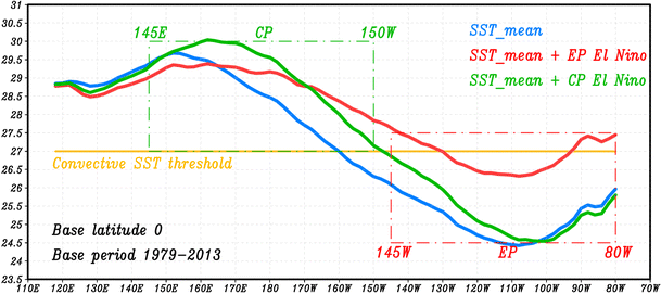
Zonal profile chart of total SST along the equatorial Pacific (0°N, 110°E–70°W) for 1979–2013. Blue line indicates the annual mean of SST. Red and green lines denote the annual mean of SST plus the double EP and CP El Niño SST anomalies shown in Fig. 1, respectively. Orange line denotes the convective SST threshold of 27 °C. Red and green dotted boxes show the longitude ranges of Niño3b and Niño4b regions
-
Since SST variances are not temporally and spatially uniform in different months and different locations (e.g., the western tropical Pacific vs. the central tropical Pacific), applying monthly normalization at each grid prior to calculating the ENSO indices is desirable.

Hence, as expected, the associated time series named as Niño3b and Niño4b (see Fig. 1; Table 1 for definition details) plotted by black curves in Fig. 1 (bottom) are directly related to RPC1 and RPC2 (red curves, Fig. 1) with robust correlations of 0.967 and 0.932, respectively.
4 Performance assessments of Niño3b and Niño4b
To judge the CP type or EP type during hybrid ENSO years, a pair of CP compass and EP compass (Table 1) is used in this study (see the flow chart shown in Fig. 4 for details): The CP compass and EP compass are respectively defined as the area mean of normalized and detrended SST anomalies over the core regions of CP El Niño and EP El Niño (see the two sky-blue boxes in Fig. 1), i.e., (160°E–180°E, 5°S–5°N) and (110°W–90°W, 5°S–5°N), and over the insignificant regions of EP El Niño and CP El Niño (Fig. 1). Figure 3 shows the phase space relationship between Niño3 and Niño4, and between Niño3b and Niño4b, for examinations of their ability to separate the ENSO types. A strong linear relationship (r = 0.75) exists between Niño3 and Niño4, as shown in Fig. 3a where many red/orange dots are mixed with each other, meaning that Niño3 and Niño4 indices may not be suitable for distinguishing the two types of El Niño. In contrast, the correlation between Niño3b and Niño4b is very small but non-orthogonal (r = 0.22, Fig. 3b). Moreover, Niño3b and Niño4b perform well in distinguishing the two types of El Niño. As seen from Fig. 3b, the red/blue and orange/green dot-clusters, to a large extent, are moved to the horizontal and vertical regions.

Phase space distribution of a normalized and detrended Niño3 and Niño4 indices in all calendar months for 1979–2013. Shown in b is the same as in a, but for Niño3b and Niño4b. Red, orange, blue, and green dots respectively indicate EP El Niño, CP El Niño, EP La Niña, and CP La Niña events identified by the method shown in Fig. 4

Flow chart identifying the EP or CP type by using normalized and detrended Niño3 and Niño4 (also Niño3b and Niño4b) with the help of EP compass and CP compass during hybrid ENSO events
Whether are there any seasonal changes in the special patterns and Niño-box locations of EP El Niño and CP El Niño? To verify the RC-REOF patterns that are directly derived from monthly successive SST data, we separately perform the same analysis on the tropical Pacific SST for each of the four seasons. Here the traditional four boreal seasons are separately defined as December–February (DJF, winter), March–May (MAM, spring), June–August (JJA, summer), and September–November (SON, autumn), in which the DJF of 1979 denotes December 1978 and January and February 1979. As noted by Marathe et al. (2015), comparison of the seasonal results provides a third independent dimension in addition to the changes in RPC and REOF, which benefits to objectively verify the physical reliability of the results from REOF.
As shown in Fig. 5, the first two RC-REOF modes of tropical Indo-Pacific SST are quasi-stable in each season from the Niño-box locations, albeit with variations in amplitude. The seasonally explained variances are shown in Table 2, which indicates comparable explained variances between EP El Niño and CP El Niño. As expected, the corresponding RPC1 and RPC2 are also directly related to Niño3b and Niño4b (Fig. 5) with significant correlations up to 0.965, 0.982, 0.950, and 0.962 for EP ENSO, and 0.932, 0.924, 0.954, and 0.950 for CP El Niño during boreal winter, spring, summer and autumn, respectively.

Same as in Fig. 1, but for seasonal RC-REOF patterns in a–b DJF, c–d MAM, e–f JJA, and g–h SON
In addition, we calculate the correlation between RPCs and 19 ENSO-related indices (Fig. 6). It is found that (1) all the EP-type indices (i.e., Niño1 + 2, Niño3, Niño3b, NCT, EI, and EPI) are highly correlated with RPC1 (Fig. 6a), and all the CP-type indices (i.e., Niño4, Niño4b, NWP, CI, CPI, EMI, and IEMI) are highly correlated with RPC2 (Fig. 6b). (2) Niño3b is most (least) significantly correlated with RPC1 (RPC2), while Niño4b is most (least) significantly correlated with RPC2 (RPC1) (Fig. 6). The above results suggest that the EP and CP ENSO patterns derived from RC-REOF are reliable, reconfirming the previous theory and advantages about REOF, especially in capturing localized modes (Lian and Chen 2012).

a Correlation between RPC1 and 19 ENSO-related indices for 1979–2013. b Is the same as in a, but for RPC2. The thick black line denotes the mean of DJF, MAM, JJA, SON and monthly correlations. The 19 indices are EP-class (Niño1 + 2, Niño3, Niño3b, NCT, EI, and EPI), hybrid-class (SOI, MEI, ONI, Niño3.4, and Niño3.4b), and CP-class (TNI, Niño4, Niño4b, NWP, CI, CPI, EMI, and IEMI), which are displayed on the x-axis from left to right. Note that Niño1 + 2, Niño3, Niño3b, Niño3.4, Niño3.4b, Niño4, and Niño4b are referred as N1 + 2, N3, N3b, N3.4, N3.4b, N4, and N4b in Figs. 6 and 14b, respectively
To confirm the above results, we further examine the seasonality of the ability of the new indices in capturing EP El Niño and CP El Niño (Figs. 7, 8). Figure 7 shows the seasonal phase space relationships between Niño3b and Niño4b to examine their ability of separating the ENSO types in each season. Correspondingly, The seasonal evolution (e.g., DJF–MAM–JJA–SON of 1979 followed by DJF–MAM–JJA–SON of 1980) of normalized and detrended SST anomalies along the equatorial central–eastern Pacific is shown in Fig. 8 to mirror the relative intensity, location, and propagation of SST anomalies, etc. It clearly reflects that the CP El Niño occurs more frequently since the 1990 (e.g., Yu et al. 2012) and the location of CP El Niño covers a broad range of longitudes with changeable anomaly centers (Capotondi et al. 2015). Inspiringly, most of EP and CP El Niño events can be well captured by Niño3b and Niño4b when comparing the seasonal types of ENSO shown in Fig. 7 and the seasonal evolution of SST anomalies shown in Fig. 8.

Same as in Fig. 3, but for a winter, b summer, c spring and d autumn during 1979–2013. The red/blue, orange/green, and gray dots indicate the EP El Niño/La Niña, CP El Niño/La Niña, and quasi-neutral states, where the number correspond to the tail of each year

Seasonal evolution of normalized and detrended SST anomaly along the equatorial central–eastern Pacific (10°S–10°N, 144°E–80°W; averaged with each three longitude grids) from DJF–SON 1979 to DJF–SON 2013. The color shading and black line are for normalized SST anomaly and the value of 1 SD, respectively
To better understand to what extent the Niño3b and Niño4b indices can depict the variability of tropical Indo-Pacific SST, we show the correlation/regression maps of SST anomalies with/onto normalized Niño3b and Niño4b, as shown in Fig. 9. Clearly, the patterns of Figs. 1 and 9 or 5 are highly similar to each other. We subsequently calculate the contribution of local variance (Fig. 10) to quantify Niño3b and Niño4b indices more intuitively. The local variance contribution is defined as the ratio of the regressed variance to the original variance at each grid (Hu et al. 2015). This analysis sheds light on a more precise contribution of Niño3b and Niño4b to the tropical Indo-Pacific SST. As shown in Fig. 10, the most eye-capturing features are the areas with yellow-to-orange shadings over EP and CP, which highlight that the local variance contribution is up to 70–95 % or so. The above results suggest that Niño3b and Niño4b are capable of distinguishing the intensity and location of the different types of ENSO SST modes and perform well in the real-time monitoring of EP and CP ENSO SST anomalies. Their unified simple, straightforward, and effective properties make them potentially valuable for both observational analysis and climate modeling.

Same as in Fig. 1 (top), but for regression/correlation on/with normalized and detrended Niño3b (left panels) and Niño4b (right panels)

Locally-explained variance contribution (10 % contour interval) defined as the ratio of regressed variance of Niño3b (left panels) and Niño4b (right panels) indices to the original variance. The black rectangular boxes (bottom) denote the Niño3.4b region (180°E–115°W, 12°S–12°N)
Given that hybrid ENSO SST anomalies inevitably appear as well, we also propose a hybrid ENSO index Niño3.4b (Table 1) defined as the same as Niño3b and Niño4b but for the region of 180°E–115°W/12°S–12°N. The coefficient of simultaneous correlation between Niño3.4b and Niño3.4 is 0.916 (0.956, 0.912, 0.909, and 0.960) for all months (DJF, MAM, JJA, and SON) for 1979–2013. It is seen from Figs. 10 and 15 that the box-Niño3.4b almost separately circles half of the variances/areas of EP and CP ENSO SST anomalies. Hence Niño3.4b is both highly and relative-equally correlated with RPC1 and RPC2 (Fig. 6a, b), whereas Niño3.4 shares more (less) signals of EP (CP) ENSO (Fig. 6a, b), indicating that Niño3.4b is more suitable for describing the hybrid ENSO SST anomalies as expected.
5 How the EP and CP ENSO events identified by Niño3b and Niño4b differ from those identified by other indices
What are the differences of EP and CP patterns identified by different types of ENSO indices? To answer the question, we examine the composite special patterns of different two types of warm and cold ENSO events. We first show the normalized time series (1979–2013) of six EP ENSO indices (i.e., Niño3, Niño3b, NCT, EI, EPI, and Niño1 + 2) and seven CP ENSO indices (i.e., Niño4, Niño4b, NWP, CI, CPI, EMI, and IEMI) in Figs. 11a and 12a, respectively. Next we select out the months when those indices exceed the ±0.7 SD (i.e., ±0.7 standard deviation). To highlight the commonality and individuality of each index, we further select out the EP-ALL events and the CP-ALL events, which are separately shown in Figs. 11b and 12b—Note that the so-called EP-ALL and CP-ALL events must together meet the following conditions of the so-called commonality:

a Monthly normalized time series of six different EP ENSO indices for 1979–2013, red/blue straight line indicates the ±0.7 SD. b Composite maps for EP El Niño events (upper) identified by the conditions of all EP ENSO indices ≥0.7 SD, and EP La Niña events (lower) identified by the conditions of all EP ENSO indices ≤−0.7 SD. c Composite maps for EP El Niño events (upper conditions: Niño3b ≥0.7 SD but the events chose for a are excluded) and EP La Niña events (bottom conditions: Niño3b ≤−0.7 SD but the events chose for a are excluded). d–h Same as in c, but for Niño3, NCT, Niño1 + 2, EI, and EPI, respectively. The numbers of warm (+) and cold (−) events are correspondingly shown in the top of each small figure, e.g., +33 and −19 for a. Regions outlined by black curves suggest that the local SST anomalies exceed the 0.5 SD

a Monthly normalized time series of seven different CP ENSO indices for 1979–2013, red/blue straight line indicates the ±0.7 SD. b Composite maps for CP El Niño events (upper) identified by the conditions of all CP ENSO indices ≥0.7 SD, and CP La Niña events (lower) identified by the conditions of all CP ENSO indices ≤−0.7 SD. c Composite maps for CP El Niño events (upper conditions: Niño4b ≥0.7 SD but the events chose for a are excluded) and CP La Niña events (bottom conditions: Niño4b ≤−0.7 SD but the events chose for a are excluded). d–i Same as in (c), but for Niño4, NWP, CI, CPI, EMI, and IEMI, respectively. The numbers of warm (+) and cold (−) events are correspondingly shown in the top of each small figure, e.g., +38 and −50 for a. Regions outlined by black curves suggest that the local SST anomalies exceed the 0.5 SD. Circles mark the same region as a reference system to highlight the differences in the CP spatial signals
-
1.
All EP ENSO indices ≥+0.7 SD for EP-ALL El Niño composites,
-
2.
All EP ENSO indices ≤−0.7 SD for EP-ALL La Niña composites,
-
3.
All CP ENSO indices ≥+0.7 SD for CP-ALL El Niño composites,
-
4.
All CP ENSO indices ≤−0.7 SD for CP-ALL La Niña composites.
Excluding the above events, if Niño3 ≥+0.7 SD in 1 month, then this month is belong to the corresponding El Niño composites; else if Niño3 ≤−0.7 SD in 1 month, then this month is belong to the corresponding La Niña composites; and vice versa for other EP and CP ENSO indices. Relevant EP and CP composite results are separately shown in Figs. 11c–h and 12c–i, which indicate the so-called individuality.
As expected, the maximum anomalies are located near the coast of South America for EP-ALL ENSO (Fig. 11a) and distinct from the CP-ALL ENSO (Fig. 12a). The individualities of Niño3, Niño3b, and NCT show good performances in capturing the EP ENSO (Fig. 11c–e), with a maximum of 50 EP El Niño events identified by Niño3 (Fig. 11d) and a maximum of 78 EP La Niña events identified by Niño3b (Fig. 11c). Note that the warm events identified by EI and EPI are more like to the CP La Niña (Fig. 11g–h), and the cold events identified by EPI are also like the CP El Niño (Fig. 11h). So the EI and EPI show significant correlations with the RPC2 (Fig. 6b).
The individualities of Niño4b, NWP, and CPI show good performances in capturing the CP ENSO (Fig. 12c, e, g), with a maximum of 89 CP El Niño and a maximum of 66 CP La Niña events identified by Niño4b (Fig. 12c). In comparison with the CP ENSO patterns identified by NWP (Fig. 12e) and CPI (Fig. 12g), the anomaly centers captured by Niño4b are located more west (Fig. 12c) and the numbers of such cases are very big (+89 vs. −66). Although the anomalies in Fig. 12c are relatively smaller than those in Fig. 12e, g, of note is that the SST variances are relatively larger over the western tropical Pacific than the central tropical Pacific (not shown). The warm events identified by Niño4 and CI are more like to the EP El Niño (Fig. 12d, f), and the cold events identified by Niño4 are also like the EP La Niña (Fig. 12d), leading to the Niño4 and CI have significant correlations with the RPC1 (Fig. 6a). Interestingly, there is no obvious negative SST anomaly over the southeast equatorial Pacific in the CP El Niño pattern identified by EMI (Fig. 12h, upper), not corresponding to the definition of EMI. Moreover, the positive and negative SST anomalies are comparable in the CP La Niña pattern identified by EMI (Fig. 12h, lower). Particularly, the cold events identified by IEMI are more like the EP El Niño (Fig. 12i), which may occur in boreal spring and summer since there are significant correlations between IEMI and RPC1 in MAM and JJA (Fig. 6a).
Anyway, no two leaves are alike. Just because the faces of ENSO are capriccioso (Capotondi et al. 2015, and see Fig. A2), the composite maps obtained from different types of ENSO indices are also changeable. Hence no ENSO index can mirror all aspects of ENSO. Researchers could choose the any index listed or not listed in the Table 1 according to individual interests, since the robustness of teleconnections may vary among various ENSO indices and different definitions inspire different understandings.
6 Interdecadal signals indirectly reflected by the evolutions of lead/lag correlation of CP ENSO and EP ENSO
Trenberth and Stepaniak (2001) used the lead/lag correlation between Nino3.4 and TNI to describe their interconnection evolutions at various leads and lags and spectacularly revealed the abrupt transition of the changes in evolution of ENSO. Accordingly, we also use the same method proposed by Trenberth and Stepaniak (2001), i.e., the 20-year running correlations of different ENSO types as a function of lead/lag month (Fig. 13), to examine the interdecadal signals indirectly reflected by such cases as the transition-in-significance or fracture of the lead/lag correlations between CP El Niño and EP El Niño.

a Leading/lagging cross correlations between Niño3b and Niño4b as a moving window of 241-month (about 20-year). The method is the same as in Trenberth and Stepaniak (2001, see their Fig. 2). Positive value-y means Niño3b leads Niño4b by y-month, and vice versa. Blue/red lines indicate absolute values exceeding 0.28 (the 5 % two-tailed significance level), and the green line is the zero. Shown in b–h are the same as in a, but for the other pairs of two types of ENSO indices as displayed in b–h
For example, one of the most prominent features contrasted by results shown in Fig. 13a, b is that the quasi-simultaneous correlation between Niño3b and Niño4b has changed from significant to unapparent since the mid-to-late 1980s, while the relationship between Niño3 and Niño4 has been always robust. The features captured by Fig. 13c are consistent with Trenberth and Stepaniak (2001, see their Fig. 2), which reflect the transition-in-significance or fracture of correlations occurred in the mid-1960s, mid-to-late 1970s, and mid-to-late 1980s, and others similar (not repeated). Compared with Fig. 13c–h that are depicted by other two types of ENSO indices, Fig. 13a (Niño3b vs. Niño4b) not only reflects the well-known “mid-to-late 1970s climate shift” but also mirrors several decadal variations of the Pacific climate regime in the mid-1960s, mid-to-late 1980s (e.g., Yu et al. 2012; Sun et al. 2015), and late-1990s (Jo et al. 2015). Meanwhile, correlations at zero lag, as shown in Fig. 13c–h, are always close to zero before the mid-1970s because the EP ENSO signal is more or less removed from these definitions of CP indices. However, this phenomenon does not exist in Fig. 13a, b (before the mid-to-late 1980s) until the frequent CP ENSO era (after the late-1980s). The phenomenon reflected by these different two types of ENSO indices can also be captured clearly (not shown) when a 15-year moving window is applied to calculate the lead/lag correlations as adopted by Ren and Jin (2011).
To validate the above-addressed four decadal-like climate shifts, we analyze the low-pass filtered time series of the Interdecadal Pacific Oscillation (IPO; Power et al. 1999; Parker et al. 2007; Henley et al. 2015) as shown in Fig. 14, and compare the correlations of 19 ENSO-related indices with the IPO index (note that all indices are monthly detrended to remove the global warming signal before calculating the correlations, as in Henley et al. 2015). It is clearly seen that the four decadal-like ENSO regime shifts act in good concert with the filtered IPO at each time when the IPO is close to zero (Fig. 14a). The feature indicates that the four decadal-like Pacific climate shifts are indeed existent. It also indicates that there may be a large difference in the relationship between the two types of ENSO even though during the “same” IPO background (e.g., the periods of 1977–1987 and 1988–1998, Fig. 14a) since Fig. 13 mirrors the significant changes in the lead/lag correlations between the different two types of El Niño (e.g., Niño3b and Niño4b, Niño3.4 and TNI, EPI and CPI, and Niño3 and EMI) in the mid-to-late 1980s. In addition, both Niño3b and Niño4b have a significant correlation above 0.35 with the IPO (Fig. 14b). The correlation between IPO and Niño3b is the highest among all EP ENSO indices, and the correlation between IPO and Niño4b is also the highest among all CP ENSO indices except Niño4 and CI (Fig. 14b). Note that CI = 1.4 × Niño4 − 0.1 × Niño1 + 2 (Table 1), almost the same as Niño4. However, the covariance between Niño4 and Niño3 is above 55 % (r = 0.75, Fig. 3a), whereas the covariance between Niño4b and Niño3b is below 5 % (r = 0.22, Fig. 3b), suggesting that Niño3b and Niño4b better reflect the different aspects of Pacific decadal signals (i.e., IPO). In addition, Niño3.4b is the best index when comparing its correlation with IPO among all indices (Fig. 14b).

a Low-pass filtered IPO time series supplied by Henley et al. (2015). b Correlations of 19 ENSO-related indices with the detrended IPO index for 1951–2014
7 Concluding remarks and discussions
Of particular interest of this study is in revisiting the spatial–temporal characteristics of the two types of El Niño, with an emphasis on development of a new pair of representative, relatively independent, and simple Niño indices for better real-time monitoring of different ENSO variations. By applying a new combined technique (named RC-REOF), the dominant modes of EP El Niño and CP El Niño are captured by using the monthly normalized tropical Pacific SST observed in recent satellite decades, with comparable explained-variance corresponding to the frequent occurrence of CP El Niño. Based on the characteristics mirrored by the two leading RC-REOF modes, Niño3b and Niño4b indices are unearthed for measuring and distinguishing the intensity and location of the SST anomalies for two types of El Niño (Figs. 1, 5). Also, the climate teleconnections (i.e., land surface temperature and precipitation) associated with Niño3b and Niño4b are distinct in each season (Figs. A3, A4), suggesting that the two new indices are potentially useful for monitoring the two types of El Niño and associated climate anomalies.
For comparison, two integrated location maps of the traditional and the new Niño SST regions have been shown in Fig. 15a, b, respectively. It is clearly seen that Niño3 and Niño4 boxes are respectively located in the EP and CP regions. However, the box-Niño4 shares part of EP ENSO signals that leads to a strong correlation (up to 0.75) between Niño3 and Niño4. The Niño3 and Niño4 boxes are equatorially symmetric, whereas EP El Niño and CP El Niño are equatorially asymmetric (e.g., Cai et al. 2015a). Hence we have defined Niño3b and Niño4b boxes as shown in Fig. 15b. One important feature of Nino4b is that off-equatorial signals are included in the calculation, which has low-frequency variability of a warming trend in nature (before being detrended, not shown), mostly corresponding to the increasing years of CP El Niño identified by Iza and Calvo (2015). This feature support the idea that CP El Niño events are getting more frequent and stronger (e.g., Lee and McPhaden 2010; Yeh et al. 2009; Yu and Kim 2013), and that local processes associated with the subtropical interannual variability over CP play a key role in the evolution of CP El Niño (Yu et al. 2010). Then, why is the region (145°E–155°E, 12°S–15°N) contained in the box-Niño4b? This is because that the box-Niño4b also shares part of warm signal of EP El Niño and the blue shading is also a part of cold signal of EP El Niño, which together play a role in helping Niño4b to offset its own EP El Niño signal. A new Niño3.4b index that is highly and relatively-equally linked to the different types of El Niño has also been proposed to descript the hybrid ENSO SST anomalies. It is seen from Fig. 15a, b that box Niño3.4 is with only a small part intersected in the key region of CP El Niño, whereas box Niño3.4b has a more balanced ratio (also see correlations shown in Fig. 6). Hence Niño3.4b is a better choice for measuring the hybrid ENSO SST anomalies.

Location of Niño SST regions: a Niño3 (5°S–5°N, 150°W–90°W), Niño4 (5°S–5°N, 160°E–150°W), Niño3.4 (5°S–5°N, 150°W–90°W); b Niño3b (12°S–5°N, 145°W–80°W), Niño4b (12°S–15°N, 145°E–150°W), and Niño3.4b (12°S–12°N, 180°E–115°W). Orange/blue shadings indicate the warm/cold parts of the main body of EP El Niño over the eastern/western tropical Pacific. Red line outlines the main body of CP El Niño. Both orange and blue shadings are intersected in the box of Niño4b, which considerably contributes to weakening the Niño3/Niño3b signal, one of areas where the Niño4b is superior to the Niño4
More inspiringly, as shown in Fig. 13a, the lead/lag interrelationship between Niño3b and Niño4b is able to mirror the recent four decadal Pacific climate shifts (i.e., the mid-1960s, mid-to-late-1980s, late-1990s, and the popular mid-to-late-1970s). Interestingly, the EPI is negatively correlated with the RPC2 (Fig. 6b) and CPI (r = −0.50 for 1979–2013) significantly. Also, the running correlations at near zero-lag revealed by Fig. 13d have experienced a transition from weak to strong since 1982/83. The reasons for this feature can be twofolds. First, the EPI is defined as the PC1 of tropical Pacific SST anomalies after deleting the signals of Niño4 (Kao and Yu 2009; Yu and Kim 2010); however, Niño3 and Niño4 share about 56.25 % covariance, which makes the corresponding positive EPI-pattern similar to the type of La Niña Modoki, and vice versa (refer to Fig. 11h). Secondly, CP El Niño occurs more frequently in the context of global warming (e.g., Lee and McPhaden 2010). Hence, the running correlation between EPI and CPI becomes more significant, which is not surprising however. After all, no ENSO index can fully reflect all aspects of ENSO due to the capriccioso faces of ENSO (Capotondi et al. 2015; Fig. A2). Consequently, the flourishing of ENSO indices (Table 1) is needed since different definitions lead to more understandings of ENSO (Figs. 11, 12) and associated climate anomalies.
References
Ashok K, Behera SK, Rao SA, Weng H, Yamagata T (2007) El Niño Modoki and its possible teleconnection. J Geophys Res 112:C11007. doi:10.1029/2006JC003798
Cai W et al (2014) Increasing frequency of extreme El Niño events due to greenhouse warming. Nat Clim Change 4:111–116. doi:10.1038/nclimate2100
Cai W et al (2015a) ENSO and greenhouse warming. Nat Clim Change 5:849–859. doi:10.1038/nclimate2743
Cai W et al (2015b) Increased frequency of extreme La Niña events under greenhouse warming. Nat Clim Change 5:132–137. doi:10.1038/nclimate2492
Capotondi A et al (2015) Understanding ENSO diversity. Bull Am Meteorol Soc 96:921–938. doi:10.1175/BAMS-D-13-00117.1
Feng J, Li J (2011) Influence of El Niño Modoki on spring rainfall over South China. J Geophys Res 116:D13102. doi:10.1029/2010JD015160
Feng J, Li J (2013) Contrasting impacts of two types of ENSO on the boreal spring Hadley circulation. J Clim 26:4773–4789. doi:10.1175/JCLI-D-12-00298.1
Fu C, Fletcher JO (1985) Two types of equatorial warming during El Niño. Chin Sci Bull 8:596–599 (in Chinese)
Fu C, Diaz HF, Fletcher JO (1986) Characteristics of the response of sea surface temperature in the central Pacific associated with warm episodes of the Southern Oscillation. Mon Weather Rev 114:1716–1739
Graf H-F (1986) On El Niño/Southern Oscillation and Northern Hemispheric temperature. Gerlands Beitr Geophys 95:63–75
Graf H-F, Zanchettin D (2012) Central Pacific El Niño, the “subtropical bridge”, and Eurasian climate. J Geophys Res 117(D1):D01102. doi:10.1029/2011JD016493
Graham NE, Barnett TP (1987) Sea surface temperature, surface wind divergence, and convection over tropical oceans. Science 238:657–659. doi:10.1126/science.238.4827.657
Ha Y, Zhong Z, Yang X, Sun Y (2013) Different Pacific Ocean warming decaying types and Northwest Pacific tropical cyclone activity. J Clim 26:8979–8994. doi:10.1175/JCLI-D-13-00097.1
Henley BJ, Gergis J, Karoly DJ, Power S, Kennedy J, Folland CK (2015) A tripole index for the Interdecadal Pacific Oscillation. Clim Dyn 45:3077–3090. doi:10.1007/s00382-015-2525-1
Horel JD (1981) A rotated principal component analysis of the interannual variability of the Northern Hemisphere 500-mb height field. Mon Weather Rev 109:2080–2092
Hu C, Yang S, Wu Q (2015) An optimal index for measuring the effect of East Asian winter monsoon on China winter temperature. Clim Dyn 45:2571–2589. doi:10.1007/s00382-015-2493-5
Huang B, Banzon VF, Freeman E, Lawrimore J, Liu W, Peterson TC, Smith TM, Thorne PW, Woodruff SD, Zhang H-M (2015) Extended reconstructed sea surface temperature version 4 (ERSST.v4). Part I: upgrades and intercomparisons. J Clim 28:911–930. doi:10.1175/JCLI-D-14-00006.1
Iza M, Calvo N (2015) Role of stratospheric sudden warmings on the response to central Pacific El Niño. Geophys Res Lett 42:2482–2489. doi:10.1002/2014GL062935
Jo H-S, Yeh S-W, Lee S-K (2015) Changes in the relationship in the SST variability between the tropical Pacific and the North Pacific across the 1998/1999 regime shift. Geophys Res Lett 42:7171–7178. doi:10.1002/2015GL065049
Kao H-Y, Yu J-Y (2009) Contrasting eastern-Pacific and central-Pacific types of ENSO. J Clim 22:615–632. doi:10.1175/2008JCLI2309.1
Karori MA, Li J, Jin F-F (2013) The asymmetric influence of the two types of El Niño and La Niña on summer rainfall over Southeast China. J Clim 26:4567–4582. doi:10.1175/JCLI-D-12-00324.1
Kim H-M, Webster PJ, Curry JA (2009) Impact of shifting patterns of Pacific Ocean warming on North Atlantic tropical cyclones. Science 325:77–80. doi:10.1126/science.1174062
Kug J-S, Jin F-F, An S-I (2009) Two types of El Niño events: cold tongue El Niño and warm pool El Niño. J Clim 22:1499–1515. doi:10.1175/2008JCLI2624.1
Larkin NK, Harrison DE (2005) On the definition of El Niño and associated seasonal average US weather anomalies. Geophys Res Lett 32:L13705
Latif M, Keenlyside NS (2009) El Niño/Southern Oscillation response to global warming. Proc Natl Acad Sci USA 106:20578–20583. doi:10.1073/pnas.0710860105
Lau K-M, Yang S (1996) The Asian monsoon and predictability of the tropical ocean-atmosphere system. Q J R Meteorol Soc 122:945–957
Lee T, McPhaden MJ (2010) Increasing intensity of El Niño in the central-equatorial Pacific. Geophys Res Lett 37:L14603
Li G, Ren B, Yang C, Zheng J (2010) Indices of El Niño and El Niño Modoki: an improved El Niño Modoki index. Adv Atmos Sci 27(5):1210–1220
Lian T, Chen D (2012) An evaluation of rotated EOF analysis and its application to tropical pacific SST variability. J Clim 25:5361–5373. doi:10.1175/JCLI-D-11-00663.1
Liu W, Huang B, Thorne PW, Banzon VF, Zhang H-M, Freeman E, Lawrimore J, Peterson TC, Smith TM, Woodruff SD (2015) Extended reconstructed sea surface temperature version 4 (ERSST.v4): part II. Parametric and structural uncertainty estimations. J Clim 28:931–951. doi:10.1175/JCLI-D-14-00007.1
López-Parages J, Rodríguez-Fonseca B, Dommenget D, Frauen C (2016) ENSO influence on the North Atlantic European climate: a non-linear and non-stationary approach. Clim Dyn. doi:10.1007/s00382-015-2951-0
Marathe S, Ashok K, Swapna P, Sabin TP (2015) Revisiting El Niño Modokis. Clim Dyn 45:3527–3545. doi:10.1007/s00382-015-2555-8
Nakamura H, Lin G, Yamagata T (1997) Decadal climate variability in the North Pacific during the recent decades. Bull Am Meteorol Soc 78:2215–2225
North GR, Bell TL, Cahalan RF, Moeng FJ (1982a) Sampling errors in the estimation of empirical orthogonal functions. Mon Weather Rev 110:699–706
North GR, Moeng FJ, Bell TL, Cahalan RF (1982b) The latitude dependence of the variance of zonally averaged quantities. Mon Weather Rev 110:319–326
Parker D et al (2007) Decadal to multidecadal variability and the climate change background. J Geophys Res 112:D18115
Power S, Casey T, Folland C, Colman A, Mehta V (1999) Inter-decadal modulation of the impact of ENSO on Australia. Clim Dyn 15(5):319–324
Rayner NA, Parker DE, Horton EB, Folland CK, Alexander LV, Rowell DP, Kent EC, Kaplan A (2003) Global analyses of sea surface temperature, sea ice, and night marine air temperature since the late nineteenth century. J Geophys Res 108(D14):4407. doi:10.1029/2002JD002670
Ren H-L, Jin F-F (2011) Niño indices for two types of ENSO. Geophys Res Lett 38:L04704. doi:10.1029/2010GL046031
Richman MB (1986) Rotation of principal components. Int J Climatol 6:293–335
Ropelewski CF, Jones PD (1987) An extension of the Tahiti–Darwin Southern Oscillation Index. Mon Weather Rev 115:2161–2165
Sardeshmukh PD, Hoskins BJ (1988) The generation of global rotational flow by steady idealized tropical divergence. J Atmos Sci 45:1228–1251
Sun J, Wu S, Ao J (2015) Role of the North Pacific sea surface temperature in the East Asian winter monsoon decadal variability. Clim Dyn. doi:10.1007/s00382-015-2805-9
Takahashi K, Montecinos A, Goubanova K, Dewitte B (2011) ENSO regimes: reinterpreting the canonical and Modoki El Niño. Geophys Res Lett 38:L10704. doi:10.1029/2011GL047364
Trenberth KE, Stepaniak DP (2001) Indices of El Niño evolution. J Clim 14:1697–1701
Vavrus S, Notaro M, Liu Z (2006) A mechanism for abrupt climate change associated with tropical Pacific SSTs. J Clim 19:242–256. doi:10.1175/JCLI3608.1
Wallace JM, Gutzler DS (1981) Teleconnections in the geopotential height field during the Northern Hemisphere winter. Mon Weather Rev 109:784–812
Wang L, Chen W, Huang R (2007) Changes in the variability of North Pacific Oscillation around 1975/1976 and its relationship with East Asian winter climate. J Geophys Res 112:D11110. doi:10.1029/2006JD008054
Wang L, Chen W, Huang R (2008) Interdecadal modulation of PDO on the impact of ENSO on the East Asian winter monsoon. Geophys Res Lett 35:L20702
Wang L, Chen W, Zhou W, Chan JCL, Barriopedro D, Huang R (2010) Effect of the climate shift around mid 1970s on the relationship between wintertime Ural blocking circulation and East Asian climate. Int J Climatol 30:153–158
Webster PJ (1995) The annual cycle and the predictability of the tropical coupled ocean–atmosphere system. Meteorol Atmos Phys 56:33–55
Webster PJ, Yang S (1992) Monsoon and ENSO: selectively interactive systems. Q J R Meteorol Soc 118:877–926
Weng H, Ashok K, Behera SK, Rao SA, Yamagata T (2007) Impacts of recent El Niño Modoki on dry/wet conditions in the Pacific rim during boreal summer. Clim Dyn 29:113–129. doi:10.1007/s00382-007-0234-0
Weng H, Behera SK, Yamagata T (2009) Anomalous winter climate conditions in the Pacific rim during recent El Niño Modoki and El Niño events. Clim Dyn 32:663–674. doi:10.1007/s00382-008-0394-6
Wolter K, Timlin MS (1998) Measuring the strength of ENSO events: How does 1997/98 rank? Weather 53:315–324
Xie F, Li J, Tian W, Feng J, Huo Y (2012) Signals of El Niño Modoki in the tropical tropopause layer and stratosphere. Atmos Chem Phys 12:5259–5273. doi:10.5194/acp-12-5259-2012
Xie F, Li J, Tian W, Li Y, Feng J (2014a) Indo-Pacific warm pool area expansion, Modoki activity, and tropical cold-point tropopause temperature variations. Sci Rep 4:4552. doi:10.1038/srep04552
Xie F, Li J, Tian W, Zhang J, Sun C (2014b) The relative impacts of El Niño Modoki, canonical El Niño, and QBO on tropical ozone changes since the 1980s. Environ Res Lett 9:064020. doi:10.1088/1748-9326/9/6/064020
Yeh S-W, Kug J-S, Dewitte B, Kwon M-H, Kirtman BP, Jin F-F (2009) El Niño in a changing climate. Nature 461:511–514. doi:10.1038/nature08316
Yu J-Y, Kao H-Y (2007) Decadal changes in ENSO persistence barrier in SST and ocean content indices: 1958–2001. J Geophys Res 112:D13106
Yu J-Y, Kim ST (2010) Identification of central-Pacific and eastern-Pacific types of ENSO in CMIP3 models. Geophys Res Lett 37:L15705
Yu J-Y, Kim ST (2011) Relationships between extratropical sea level pressure variations and the central Pacific and eastern Pacific types of ENSO. J Clim 24:708–720. doi:10.1175/2010JCLI3688.1
Yu J-Y, Kim ST (2013) Identifying the types of major El Niño events since 1870. Int J Climatol 33:2105–2112. doi:10.1002/joc.3575
Yu J-Y, Zou Y (2013) The enhanced drying effect of central-Pacific El Niño on US winter. Environ Res Lett 8:014019. doi:10.1088/1748-9326/8/1/014019
Yu J-Y, Kao H-Y, Lee T (2010) Subtropics-related interannual sea surface temperature variability in the central equatorial Pacific. J Clim 23:2869–2884. doi:10.1175/2010JCLI3171.1
Yu J-Y, Zou Y, Kim ST, Lee T (2012) The changing impact of El Niño on US winter temperatures. Geophys Res Lett 39:L15702. doi:10.1029/2012GL052483
Yuan Y, Yang S (2012) Impacts of different types of El Niño on the East Asian climate: focus on ENSO cycles. J Clim 25:7702–7777
Acknowledgments
The study was supported by the National Key Scientific Research Plan of China (Grants 2012CB956002 and 2014CB953900), the National Natural Science Foundation of China (Grants 41375076 and 41375081), the China Special Fund for Meteorological Research in the Public Interest (Grant 201206038), the LASW State Key Laboratory Special Fund (2013LASW-A05), and the Jiangsu Collaborative Innovation Center for Climate Change. Calculations for this study were supported by the China National Supercomputer Center in Guangzhou.
Author information
Authors and Affiliations
Corresponding author
Electronic supplementary material
Below is the link to the electronic supplementary material.
Rights and permissions
About this article

Cite this article
Hu, C., Yang, S., Wu, Q. et al. Reinspecting two types of El Niño: a new pair of Niño indices for improving real-time ENSO monitoring. Clim Dyn 47, 4031–4049 (2016). https://doi.org/10.1007/s00382-016-3059-x
Received:
Accepted:
Published:
Issue Date:
DOI: https://doi.org/10.1007/s00382-016-3059-x