Approximation Spaces of Deep Neural Networks

Abstract

We study the expressivity of deep neural networks. Measuring a network’s complexity by its number of connections or by its number of neurons, we consider the class of functions for which the error of best approximation with networks of a given complexity decays at a certain rate when increasing the complexity budget. Using results from classical approximation theory, we show that this class can be endowed with a (quasi)-norm that makes it a linear function space, called approximation space. We establish that allowing the networks to have certain types of “skip connections” does not change the resulting approximation spaces. We also discuss the role of the network’s nonlinearity (also known as activation function) on the resulting spaces, as well as the role of depth. For the popular ReLU nonlinearity and its powers, we relate the newly constructed spaces to classical Besov spaces. The established embeddings highlight that some functions of very low Besov smoothness can nevertheless be well approximated by neural networks, if these networks are sufficiently deep.

1 Introduction

Today, we witness a worldwide triumphant march of deep neural networks, impacting not only various application fields, but also areas in mathematics such as inverse problems. Originally, neural networks were developed by McCulloch and Pitts [48] in 1943 to introduce a theoretical framework for artificial intelligence. At that time, however, the limited amount of data and the lack of sufficient computational power only allowed the training of shallow networks, that is, networks with only few layers of neurons, which did not lead to the anticipated results. The current age of big data and the significantly increased computer performance now make the application of deep learning algorithms feasible, leading to the successful training of very deep neural networks. For this reason, neural networks have seen an impressive comeback. The list of important applications in public life ranges from speech recognition systems on cell phones over self-driving cars to automatic diagnoses in healthcare. For applications in science, one can witness a similarly strong impact of deep learning methods in research areas such as quantum chemistry [61] and molecular dynamics [47], often allowing to resolve problems which were deemed unreachable before. This phenomenon is manifested similarly in certain fields of mathematics, foremost in inverse problems [2, 10], but lately also, for instance, in numerical analysis of partial differential equations [8].

Yet, most of the existing research related to deep learning is empirically driven and a profound and comprehensive mathematical foundation is still missing, in particular for the previously mentioned applications. This poses a significant challenge not only for mathematics itself, but in general for the “safe” applicability of deep neural networks [22].

A deep neural network in mathematical terms is a tuple

$$\begin{aligned} \Phi = \big ( (T_1, \alpha _1), \dots , (T_L, \alpha _L) \big ) \end{aligned}$$

(1.1)

consisting of affine-linear maps $T_\ell : {\mathbb {R}}^{N_{\ell - 1}} \rightarrow {\mathbb {R}}^{N_\ell }$ (hence $T_\ell (x) = A_\ell \, x + b_\ell$ for appropriate matrices $A_\ell$ and vectors $b_\ell$, often with a convolutional or Toeplitz structure) and of nonlinearities $\alpha _{\ell }: {\mathbb {R}}^{N_{\ell }} \rightarrow {\mathbb {R}}^{N_{\ell }}$ that typically encompass componentwise rectification, possibly followed by a pooling operation.

The tuple in (1.1) encodes the architectural components of the neural network, where L denotes the number of layers of the network, while $L-1$ is the number of hidden layers. The highly structured function ${\mathtt {R}}(\Phi )$ implemented by such a network $\Phi$ is then defined by applying the different maps in an iterative (layer-wise) manner; precisely,

$$\begin{aligned}&{\mathtt {R}}(\Phi ) : {\mathbb {R}}^{N_0} \rightarrow {\mathbb {R}}^{N_L}, \quad \text {with} \quad {\mathtt {R}}(\Phi ) := \alpha _L \circ T_L \circ \cdots \circ \alpha _1 \circ T_1 . \end{aligned}$$

We call this function the realization of the deep neural network $\Phi$. It is worth pointing out that most of the literature calls this function itself the neural network; one can, however—depending on the choice of the activation functions—imagine the same function being realized by different architectural components, so that it would not make sense, for instance, to speak of the number of layers of ${\mathtt {R}}(\Phi )$; this is only well defined when we talk about $\Phi$ itself. The complexity of a neural network can be captured by various numbers such as the depth L, the number of hidden neurons $N(\Phi ) = \sum _{\ell =1}^{L-1} N_{\ell }$, or the number of connections (also called the connectivity, or the number of weights) given by $W(\Phi ) = \sum _{\ell = 1}^{L} \Vert A_\ell \Vert _{\ell ^0}$, where $\Vert A_\ell \Vert _{\ell ^0}$ denotes the number of nonzero entries of the matrix $A_\ell$.

From a mathematical perspective, the central task of a deep neural network is to approximate a function $f : {\mathbb {R}}^{N_0} \rightarrow {\mathbb {R}}^{N_L}$, which, for instance, encodes a classification problem. Given a training data set $\big ( x_i,f(x_i) \big )_{i=1}^m$, a loss function ${\mathcal {L}} : {\mathbb {R}}^{N_L} \times {\mathbb {R}}^{N_L} \rightarrow {\mathbb {R}}$, and a regularizer ${\mathcal {P}}$, which imposes, for instance, sparsity conditions on the weights of the neural network $\Phi$, solving the optimization problem

$$\begin{aligned} \min _{\Phi } \sum _{i=1}^m {\mathcal {L}} \big ( {\mathtt {R}}(\Phi )(x_i),f(x_i) \big ) + \lambda {\mathcal {P}}(\Phi ), \end{aligned}$$

(1.2)

typically through a variant of stochastic gradient descent, yields a learned neural network ${\widehat{\Phi }}$. The objective is to achieve ${\mathtt {R}}({\widehat{\Phi }}) \approx f$, which is only possible if the function f can indeed be well approximated by (the realization of) a network with the prescribed architecture. Various theoretical results have already been published to establish the ability of neural networks—often with specific architectural constraints—to approximate functions from certain function classes; this is referred to as analyzing the expressivity of neural networks. However, the fundamental question asking which function spaces are truly natural for deep neural networks has never been comprehensively addressed. Such an approach may open the door to a novel viewpoint and lead to a refined understanding of the expressive power of deep neural networks.

In this paper, we introduce approximation spaces associated with neural networks. This leads to an extensive theoretical framework for studying the expressivity of deep neural networks, allowing us also to address questions such as the impact of the depth and of the activation function, or of so-called (and widely used) skip connections on the approximation power of deep neural networks.

1.1 Expressivity of Deep Neural Networks

The first theoretical results concerning the expressivity of neural networks date back to the early 90s, at that time focusing on shallow networks, mainly in the context of the universal approximation theorem [16, 35, 36, 43]. The breakthrough result of the ImageNet competition in 2012 [38] and the ensuing worldwide success story of neural networks have brought renewed interest to the study of neural networks, now with an emphasis on deep networks. The surprising effectiveness of such networks in applications has motivated the study of the effect of depth on the expressivity of these networks. Questions related to the learning phase are of a different nature, focusing on aspects of statistical learning and optimization, and hence constitute a different research field.

Let us recall some of the key contributions in the area of expressivity, in order to put our results into perspective. The universal approximation theorems by Hornik [35] and Cybenko [16] can be counted as a first highlight, stating that neural networks with only one hidden layer can approximate continuous functions on compact sets arbitrarily well. Examples of further work in this early stage, hence focusing on networks with a single hidden layer, are approximation error bounds in terms of the number of neurons for functions with bounded first Fourier moments [5, 6], the failure of those networks to provide localized approximations [13], a fundamental lower bound on approximation rates [12, 18], and the approximation of smooth/analytic functions [50, 52]. Some of the early contributions already study networks with multiple hidden layers, such as [29] for approximating continuous functions, and [53] for approximating functions together with their derivatives. Also, [13] which shows in certain instances that deep networks can perform better than single-hidden-layer networks can be counted toward this line of research. For a survey of those early results, we refer to [24, 57].

More recent work focuses predominantly on the analysis of the effect of depth. Some examples—again without any claim of completeness—are [23], in which a function is constructed which cannot be expressed by a small two-layer network, but which is implemented by a three-layer network of low complexity, or [51] which considers so-called compositional functions, showing that such functions can be approximated by neural networks without suffering from the curse of dimensionality. A still different viewpoint is taken in [14, 15], which focus on a similar problem as [51] but attacking it by utilizing results on tensor decompositions. Another line of research aims to study the approximation rate when approximating certain function classes by neural networks with growing complexity [9, 49, 55, 62, 68].

1.2 The Classical Notion of Approximation Spaces

In classical approximation theory, the notion of approximation spaces refers to (quasi)-normed spaces that are defined by their elements satisfying a specific decay of a certain approximation error; see, for instance, [21] In this introduction, we will merely sketch the key construction and properties; we refer to Sect. 3 for more details.

Let X be a quasi-Banach space equipped with the quasi-norm $\Vert \cdot \Vert _{X}$. Furthermore, here, as in the rest of the paper, let us denote by ${\mathbb {N}}= \{1,2,\ldots \}$ the set of natural numbers and write ${\mathbb {N}}_{0} = \{0\} \cup {\mathbb {N}}$, ${\mathbb {N}}_{\ge m} = \{n \in {\mathbb {N}}, n \ge m\}$. For a prescribed family $\Sigma = (\Sigma _{n})_{n \in {\mathbb {N}}_{0}}$ of subsets $\Sigma _{n} \subset X$, one aims to classify functions $f \in X$ by the decay (as $n \rightarrow \infty$) of the error of best approximation by elements from $\Sigma _{n}$, given by $E(f,\Sigma _{n})_X :=\inf _{g \in \Sigma _{n}} \Vert f - g \Vert _{X}$. The desired rate of decay of this error is prescribed by a discrete weighted $\ell ^q$-norm, where the weight depends on the parameter $\alpha > 0$. For $q = \infty$, this leads to the class

$$\begin{aligned} A_\infty ^\alpha (X,\Sigma ) := \Big \{ f \in X \, : \, \sup _{n \ge 1} \,\, [n^{\alpha } \cdot E(f,\Sigma _{n-1})_{X}] < \infty \Big \} . \end{aligned}$$

Thus, intuitively speaking, this class consists of those elements of X for which the error of best approximation by elements of $\Sigma _{n}$ decays at least as ${\mathcal {O}}(n^{-\alpha })$ for $n \rightarrow \infty$. This general philosophy also holds for the more general classes , $q > 0$.

If the initial family $\Sigma$ of subsets of X satisfies some quite natural conditions, more precisely $\Sigma _0 = \{0\}$, each $\Sigma _n$ is invariant to scaling, $\Sigma _n \subset \Sigma _{n+1}$, and the union $\bigcup _{n \in {\mathbb {N}}_0} \Sigma _n$ is dense in X, as well as the slightly more involved condition that $\Sigma _n + \Sigma _n \subset \Sigma _{cn}$ for some fixed $c \in {\mathbb {N}}$, then an abundance of results are available for the approximation classes . In particular, turns out to be a proper linear function space, equipped with a natural (quasi)-norm. Particular highlights of the theory are various embedding and interpolation results between the different approximation spaces.

1.3 Our Contribution

We introduce a novel perspective on the study of expressivity of deep neural networks by introducing the associated approximation spaces and investigating their properties. This is in contrast with the usual approach of studying the approximation fidelity of neural networks on classical spaces. We utilize this new viewpoint for deriving novel results on, for instance, the impact of the choice of activation functions and the depth of the networks.

Given a so-called (nonlinear) activation function $\varrho : {\mathbb {R}}\rightarrow {\mathbb {R}}$, a classical setting is to consider nonlinearities $\alpha _\ell$ in (1.1) corresponding to a componentwise application of the activation function for each hidden layer $1 \le \ell < L$, and $\alpha _{L}$ being the identity. We refer to networks of this form as strict $\varrho$-networks. To introduce a framework of sufficient flexibility, we also consider nonlinearities where for each component either $\varrho$ or the identity is applied. We refer to such networks as generalized $\varrho$-networks; the realizations of such generalized networks include various function classes such as multilayer sparse linear transforms [41], networks with skip connections [54], ResNets [32, 67], or U-nets [58].

Let us now explain how we utilize this framework of approximation spaces. Our focus will be on approximation rates in terms of growing complexity of neural networks, which we primarily measure by their connectivity, since this connectivity is closely linked to the number of bytes needed to describe the network, and also to the number of floating point operations needed to apply the corresponding function to a given input. This is in line with recent results [9, 55, 68] which explicitly construct neural networks that reach an optimal approximation rate for very specific function classes, and in contrast to most of the existing literature focusing on complexity measured by the number of neurons. We also consider the approximation spaces for which the complexity of the networks is measured by the number of neurons.

In addition to letting the number of connections or neurons tend to infinity while keeping the depth of the networks fixed, we also allow the depth to evolve with the number of connections or neurons. To achieve this, we link both by a non-decreasing depth-growth function ${\mathscr {L}}: {\mathbb {N}}\rightarrow {\mathbb {N}}\cup \{ \infty \}$, where we allow the possibility of not restricting the number of layers when ${\mathscr {L}}(n) = \infty$. We then consider the function families $\mathtt {W}_n(\Omega \rightarrow {\mathbb {R}}^{k},\varrho , {\mathscr {L}})$ (resp. $\mathtt {N}_n(\Omega \rightarrow {\mathbb {R}}^{k},\varrho , {\mathscr {L}})$) made of all restrictions to a given subset $\Omega \subseteq {\mathbb {R}}^{d}$ of functions which can be represented by (generalized) $\varrho$-networks with input/output dimensions d and k, at most n nonzero connection weights (resp. at most n hidden neurons), and at most ${\mathscr {L}}(n)$ layers. Finally, given a space X of functions $\Omega \rightarrow {\mathbb {R}}^{k}$, we will use the sets (resp. ) to define the associated approximation spaces. Typical choices for X are

(1.3)

with the space of uniformly continuous functions on $\Omega$ that vanish at infinity, equipped with the supremum norm. For ease of notation, we will sometimes also write , and (resp. ).

Let us now give a coarse overview of our main results, which we are able to derive with our choice of approximation spaces based on or .

1.3.1 Core properties of the novel Approximation Spaces

We first prove that each of these two families $\Sigma = (\Sigma _n)_{n \in {\mathbb {N}}_0}$ satisfies the necessary requirements for the associated approximation spaces —which we denote by and , respectively—to be amenable to various results from approximation theory. Under certain conditions on $\varrho$ and ${\mathscr {L}}$, Theorem 3.27 shows that these approximation spaces are even equipped with a convenient (quasi-)Banach spaces structure. The spaces and are nested (Lemma 3.9) and do not generally coincide (Lemma 3.10).

To prepare the ground for the analysis of the impact of depth, we then prove nestedness with respect to the depth growth function. In slightly more detail, we identify a partial order $\preceq$ and an equivalence relation $\sim$ on depth growth functions such that the following holds (Lemma 3.12 and Theorem 3.13):

• (1) If ${\mathscr {L}}_{1} \preceq {\mathscr {L}}_{2}$, then for any $\alpha$, q, X and $\varrho$; and

• (2) if ${\mathscr {L}}_{1} \sim {\mathscr {L}}_{2}$, then for any $\alpha$, q, X and $\varrho$.

The same nestedness results hold for the spaces . Slightly surprising and already insightful might be that under mild conditions on the activation function $\varrho$, the approximation classes for strict and generalized $\varrho$-networks are in fact identical, allowing to derive the conclusion that their expressivities coincide (see Theorem 3.8).

1.3.2 Approximation Spaces Associated with ReLU Networks

The rectified linear unit (ReLU) and its powers of exponent $r \in {\mathbb {N}}$—in spline theory better known under the name of truncated powers [21, Chapter 5, Equation (1.1)]— are defined by

$$\begin{aligned} \varrho _r : {\mathbb {R}}\rightarrow {\mathbb {R}}, x \mapsto (x_{+})^{r}, \end{aligned}$$

where $x_{+} = \max \{ 0,x \} = \varrho _{1}(x)$, with the ReLU activation function being $\varrho _{1}$. Considering these activation functions is motivated practically by the wide use of the ReLU [42], as well as theoretically by the existence [45, Theorem 4] of pathological activation functions giving rise to trivial—too rich—approximation spaces that satisfy , for all $\alpha ,q$. In contrast, the classes associated with $\varrho _{r}$-networks are non-trivial for $p \in (0,\infty ]$ (Theorem 4.16). Moreover, strict and generalized $\varrho _{r}$-networks yield identical approximation classes for any subset $\Omega \subseteq {\mathbb {R}}^d$ of nonzero measure (even unbounded), for any $p \in (0,\infty ]$ (Theorem 4.2). Furthermore, for any $r \in {\mathbb {N}}$, these approximation classes are (quasi-)Banach spaces (Theorem 4.2), as soon as

$$\begin{aligned} L := \sup _{n \in {\mathbb {N}}} {\mathscr {L}}(n) \ge {\left\{ \begin{array}{ll} 2, &{}\quad \text {if}\ \Omega \ \text {is bounded or }\ d=1, \\ 3, &{}\quad \text {otherwise.} \end{array}\right. }. \end{aligned}$$

The expressivity of networks with more general activation functions can be related to that of $\varrho _{r}$-networks (see Theorem 4.7) in the following sense: If $\varrho$ is continuous and piecewise polynomial of degree at most r, then its approximation spaces are contained in those of $\varrho _{r}$-networks. In particular, if $\Omega$ is bounded or if ${\mathscr {L}}$ satisfies a certain growth condition, then for $s,r \in {\mathbb {N}}$ such that $1 \le s \le r$

Also, if $\varrho$ is a spline of degree r and not a polynomial, then its approximation spaces match those of $\varrho _{r}$ on bounded $\Omega$. In particular, on a bounded domain $\Omega$, the spaces associated with the leaky ReLU [44], the parametric ReLU [33], the absolute value (as, e.g., in scattering transforms [46]), and the soft-thresholding activation function [30] are all identical to the spaces associated with the ReLU.

Studying the relation of approximation spaces of $\varrho _{r}$-networks for different r, we derive the following statement as a corollary (Corollary 4.14) of Theorem 4.7: Approximation spaces of $\varrho _{2}$-networks and $\varrho _{r}$-networks are equal for $r \ge 2$ when ${\mathscr {L}}$ satisfies a certain growth condition, showing a saturation from degree 2 on. Given this growth condition, for any $r \ge 2$, we obtain the following diagram:

1.3.3 Relation to Classical Function Spaces

Focusing still on ReLU networks, we show that ReLU networks of bounded depth approximate $C_{c}^{3}(\Omega )$ functions at bounded rates (Theorem 4.17) in the sense that, for open $\Omega \subset {\mathbb {R}}^d$ and $L := \sup _{n} {\mathscr {L}}(n) < \infty$, we prove

As classical function spaces (e.g., Sobolev, Besov) intersect $C^{3}_{c}(\Omega )$ non-trivially, they can only embed into or if the networks are somewhat deep ($L \ge 1 + \alpha /2$ or $\lfloor L/2 \rfloor \ge \alpha /2$, respectively), giving some insight about the impact of depth on the expressivity of neural networks.

We then study relations to the classical Besov spaces ${B^{s}_{\sigma ,\tau } (\Omega ) := B^s_{\tau }(L_\sigma (\Omega ;{\mathbb {R}}))}$. We establish both direct estimates—that is, embeddings of certain Besov spaces into approximation spaces of $\varrho _{r}$-networks—and inverse estimates— that is, embeddings of the approximation spaces into certain Besov spaces.

The main result in the regime of direct estimates is Theorem 5.5 showing that if $\Omega \subset {\mathbb {R}}^d$ is a bounded Lipschitz domain, if $r \ge 2$, and if $L := \sup _{n \in {\mathbb {N}}} {\mathscr {L}}(n)$ satisfies $L \ge 2 + 2 \lceil \log _2 d \rceil$, then

(1.4)

For large input dimensions d, however, the condition $L \ge 2 + 2 \lceil \log _2 d \rceil$ is only satisfied for quite deep networks. In the case of more shallow networks with $L \ge 3$, the embedding (1.4) still holds (for any $r \in {\mathbb {N}}$), but is only established for $0< \alpha < \tfrac{\min \{ 1, p^{-1} \}}{d}$. Finally, in case of $d = 1$, the embedding (1.4) is valid as soon as $L \ge 2$ and $r \ge 1$.

Regarding inverse estimates, we first establish limits on possible embeddings (Theorem 5.7). Precisely, for $\Omega = (0,1)^{d}$ and any $r \in {\mathbb {N}}$, $\alpha ,s \in (0,\infty )$, and $\sigma , \tau \in (0,\infty ]$ we have, with $L := \sup _{n} {\mathscr {L}}(n) \ge 2$:

• if $\alpha < \lfloor L/2\rfloor \cdot \min \{ s, 2 \}$ then does not embed into $B^{s}_{\sigma ,\tau } (\Omega )$;

• if $\alpha < (L-1) \cdot \min \{ s, 2 \}$ then does not embed into $B^{s}_{\sigma ,\tau } (\Omega )$.

A particular consequence is that for unbounded depth $L = \infty$, none of the spaces , can embed into any Besov space of strictly positive smoothness $s>0$.

For scalar input dimension $d=1$, an embedding into a Besov space with the relation $\alpha = \lfloor L/2 \rfloor \cdot s$ (respectively, $\alpha = (L-1) \cdot s$) is indeed achieved for $X = L_{p}( (0,1) )$, $0< p < \infty$, $r \in {\mathbb {N}}$, (Theorem 5.13):

1.4 Expected Impact and Future Directions

We anticipate our results to have an impact in a number of areas that we now describe together with possible future directions:

• Theory of Expressivity We introduce a general framework to study approximation properties of deep neural networks from an approximation space viewpoint. This opens the door to transfer various results from this part of approximation theory to deep neural networks. We believe that this conceptually new approach in the theory of expressivity will lead to further insight. One interesting topic for future investigation is, for instance, to derive a finer characterization of the spaces , , for $r \in \{1,2\}$ (with some assumptions on ${\mathscr {L}}$).

  Our framework is amenable to various extensions; for example, the restriction to convolutional weights would allow a study of approximation spaces of convolutional neural networks.

• Statistical Analysis of Deep Learning Approximation spaces characterize fundamental trade-offs between the complexity of a network architecture and its ability to approximate (with proper choices of parameter values) a given function f. In statistical learning, a related question is to characterize which generalization bounds (also known as excess risk guarantees) can be achieved when fitting network parameters using m independent training samples. Some “oracle inequalities” [60] of this type have been recently established for idealized training algorithms minimizing the empirical risk (1.2). Our framework in combination with existing results on the VC dimension of neural networks [7] is expected to shed new light on such generalization guarantees through a generic approach encompassing various types of constraints on the considered architecture.

• Design of Deep Neural Networks—Architectural Guidelines Our results reveal how the expressive power of a network architecture may be impacted by certain choices such as the presence of certain types of skip connections or the selected activation functions. Thus, our results provide indications on how a network architecture may be adapted without hurting its expressivity, in order to get additional degrees of freedom to ease the task of optimization-based learning algorithms and improve their performance. For instance, while we show that generalized and strict networks have (under mild assumptions on the activation function) the same expressivity, we have not yet considered so-called ResNet architectures. Yet, the empirical observation that a ResNet architecture makes it easier to train deep networks [32] calls for a better understanding of the relations between the corresponding approximations classes.

1.5 Outline

The paper is organized as follows.

Section 2 introduces our notations regarding neural networks and provides basic lemmata concerning the “calculus” of neural networks. The classical notion of approximation spaces is reviewed in Sect. 3, and therein also specialized to the setting of approximation spaces of networks, with a focus on approximation in $L_p$ spaces. This is followed by Sect. 4, which concentrates on $\varrho$-networks with $\varrho$ the so-called ReLU or one of its powers. Finally, Sect. 5 studies embeddings between (resp. ) and classical Besov spaces, with .

2 Neural Networks and Their Elementary Properties

In this section, we formally introduce the definition of neural networks used throughout this paper and discuss the elementary properties of the corresponding sets of functions.

2.1 Neural Networks and Their Main Characteristics

Definition 2.1

(Neural network) Let $\varrho : {\mathbb {R}}\rightarrow {\mathbb {R}}$. A (generalized) neural network with activation function $\varrho$ (in short: a $\varrho$-network) is a tuple $\big ( (T_1, \alpha _1), \dots , (T_L, \alpha _L) \big )$, where each $T_\ell : {\mathbb {R}}^{N_{\ell - 1}} \rightarrow {\mathbb {R}}^{N_\ell }$ is an affine-linear map, $\alpha _L = \mathrm {id}_{{\mathbb {R}}^{N_L}}$, and each function $\alpha _\ell : {\mathbb {R}}^{N_\ell }\rightarrow {\mathbb {R}}^{N_\ell }$ for $1 \le \ell < L$ is of the form $\alpha _\ell = \bigotimes _{j = 1}^{N_\ell } \varrho _j^{(\ell )}$ for certain $\varrho _j^{(\ell )} \in \{\mathrm {id}_{{\mathbb {R}}}, \varrho \}$. Here, we use the notation

$$\begin{aligned}&\bigotimes _{j=1}^n \theta _j : X_1 \times \cdots \times X_n \rightarrow Y_1 \times \cdots \times Y_n,\\&\quad (x_1,\dots ,x_n) \mapsto \big ( \theta _1 (x_1), \dots , \theta _n (x_n) \big ) \, \text { for } \, \theta _j : X_j \rightarrow Y_j . \blacktriangleleft \end{aligned}$$

Definition 2.2

A $\varrho$-network as above is called strict if $\varrho _j^{(\ell )} = \varrho$ for all $1 \le \ell < L$ and $1 \le j \le N_\ell$. $\blacktriangleleft$

Definition 2.3

(Realization of a network) The realization ${\mathtt {R}}(\Phi )$ of a network ${\Phi = \big ( (T_1, \alpha _1), \dots , (T_L, \alpha _L) \big )}$ as above is the function

$$\begin{aligned} {\mathtt {R}}(\Phi ) : {\mathbb {R}}^{N_0} \rightarrow {\mathbb {R}}^{N_L} , \quad \text {with} \quad {\mathtt {R}}(\Phi ) := \alpha _L \circ T_L \circ \cdots \circ \alpha _1 \circ T_1 . \blacktriangleleft \end{aligned}$$

The complexity of a neural network is characterized by several features.

Definition 2.4

(Depth, number of hidden neurons, number of connections) Consider a neural network $\Phi = \big ( (T_1, \alpha _1), \dots , (T_L, \alpha _L) \big )$ with $T_\ell : {\mathbb {R}}^{{N_{\ell - 1}}} \rightarrow {\mathbb {R}}^{N_\ell }$ for $1 \le \ell \le L$.

• The input-dimension of $\Phi$ is ${d_{\mathrm {in}}}(\Phi ) := N_0 \in {\mathbb {N}}$, its output-dimension is ${d_{\mathrm {out}}}(\Phi ) := N_L \in {\mathbb {N}}$.

• The depth of $\Phi$ is $L(\Phi ) := L \in {\mathbb {N}}$, corresponding to the number of (affine) layers of $\Phi$.

  We remark that with these notations, the number of hidden layers is $L-1$.

• The number of hidden neurons of $\Phi$ is $N(\Phi ) := \sum _{\ell = 1}^{L-1} N_\ell \in {\mathbb {N}}_0$;

• The number of connections (or number of weights) of $\Phi$ is $W(\Phi ) := \sum _{\ell = 1}^{L} \Vert T_\ell \Vert _{\ell ^0} \in {\mathbb {N}}_0$, with ${\Vert T\Vert _{\ell ^0} := \Vert A\Vert _{\ell ^{0}}}$ for an affine map $T: x \mapsto A x + b$ with A some matrix and b some vector; here, $\Vert \cdot \Vert _{\ell ^{0}}$ counts the number of nonzero entries in a vector or a matrix. $\blacktriangleleft$

Remark 2.5

If $W(\Phi ) = 0$, then ${\mathtt {R}}(\Phi )$ is constant (but not necessarily zero), and if $N(\Phi )=0$, then ${\mathtt {R}}(\Phi )$ is affine-linear (but not necessarily zero or constant). $\blacklozenge$

Unlike the notation used in [9, 55], which considers $W_0 (\Phi ) := \sum _{\ell = 1}^L (\Vert A^{(\ell )}\Vert _{\ell ^0} + \Vert b^{(\ell )}\Vert _{\ell ^0})$ where ${T_\ell \, x = A^{(\ell )} x + b^{(\ell )}}$, Definition 2.4 only counts the nonzero entries of the linear part of each $T_\ell$, so that $W(\Phi ) \le W_{0}(\Phi )$. Yet, as shown with the following lemma, both definitions are in fact equivalent up to constant factors if one is only interested in the represented functions. The proof is in Appendix A.1.

Lemma 2.6

For any network $\Phi$, there is a “compressed” network ${\widetilde{\Phi }}$ with ${\mathtt {R}}( {\widetilde{\Phi }} ) = {\mathtt {R}}(\Phi )$ such that $L({\widetilde{\Phi }}) \le L(\Phi )$, $N({\widetilde{\Phi }} \,) \le N(\Phi )$, and

$$\begin{aligned} W({\widetilde{\Phi }}) \le W_0 ({\widetilde{\Phi }} \,) \le {d_{\mathrm {out}}}(\Phi ) + 2 \cdot W(\Phi ) . \end{aligned}$$

The network ${\widetilde{\Phi }}$ can be chosen to be strict if $\Phi$ is strict. $\blacktriangleleft$

Remark 2.7

The reason for distinguishing between a neural network and its associated realization is that for a given function $f : {\mathbb {R}}^d\rightarrow {\mathbb {R}}^k$, there might be many different neural networks $\Phi$ with $f = {\mathtt {R}}(\Phi )$, so that talking about the number of layers, neurons, or weights of the function f is not well defined, whereas these notions certainly make sense for neural networks as defined above. A possible alternative would be to define, for example,

$$\begin{aligned} L(f) := \min \big \{ L(\Phi ) \, : \, \Phi \text { neural network with } {\mathtt {R}}(\Phi ) = f \big \}, \end{aligned}$$

and analogously for N(f) and W(f); but this has the considerable drawback that it is not clear whether there is a neural network $\Phi$ that simultaneously satisfies, e.g., $L(\Phi ) = L(f)$ and $W(\Phi ) = W(f)$. Because of these issues, we prefer to properly distinguish between a neural network and its realization.$\blacklozenge$

Remark 2.8

Some of the conventions in the above definitions might appear unnecessarily complicated at first sight, but they have been chosen after careful thought. In particular:

• Many neural network architectures used in practice use the same activation function for all neurons in a common layer. If this choice of activation function even stays the same across all layers—except for the last one—one obtains a strict neural network.

• In applications, network architectures very similar to our “generalized” neural networks are used; examples include residual networks (also called “ResNets,” see [32, 67]), and networks with skip connections [54].

• As expressed in Sect. 2.3, the class of realizations of generalized neural networks admits nice closure properties under linear combinations and compositions of functions. Similar closure properties do in general not hold for the class of strict networks.

• The introduction of generalized networks will be justified in Sect. 3.3, where we show that if one is only interested in approximation theoretic properties of the respective function class, then—at least on bounded domains $\Omega \subset {\mathbb {R}}^d$ for “generic” $\varrho$, but also on unbounded domains for the ReLU activation function and its powers—generalized networks and strict networks have identical properties. $\blacklozenge$

2.2 Relations Between Depth, Number of Neurons, and Number of Connections

We now investigate the relationships between the quantities describing the complexity of a neural network $\Phi = \big ( (T_1,\alpha _1), \dots , (T_L, \alpha _L) \big )$ with $T_\ell : {\mathbb {R}}^{N_{\ell - 1}} \rightarrow {\mathbb {R}}^{N_\ell }$.

Given the number of (hidden) neurons of the network, the other quantities can be bounded. Indeed, by definition we have $N_\ell \ge 1$ for all $1 \le \ell \le L-1$; therefore, the number of layers satisfies

$$\begin{aligned} L(\Phi ) = 1+\sum _{\ell = 1}^{L-1} 1 \le 1+ \sum _{\ell = 1}^{L-1} N_\ell = 1+ N(\Phi ) . \end{aligned}$$

(2.1)

Similarly, as $\Vert T_{\ell }\Vert _{\ell ^{0}} \le N_{\ell -1} N_{\ell }$ for each $1 \le \ell < L$, we have

$$\begin{aligned} W(\Phi )= & {} \sum _{\ell = 1}^{L} \Vert T_{\ell }\Vert _{\ell ^{0}} \le \sum _{\ell = 1}^{L} N_{\ell -1} N_{\ell } \le \sum _{\ell '=0}^{L-1}\sum _{\ell =1}^{L} N_{\ell '}N_{\ell } \nonumber \\= & {} (d_{\mathrm {in}} (\Phi ) +N(\Phi )) (N(\Phi ) + d_{\mathrm {out}}(\Phi )), \end{aligned}$$

(2.2)

showing that $W(\Phi ) = {\mathcal {O}}([N(\Phi )]^2 + d k)$ for fixed input and output dimensions d, k. When $L(\Phi )=2$, we have in fact $W(\Phi ) = \Vert T_{1}\Vert _{\ell ^{0}}+\Vert T_{2}\Vert _{\ell ^{0}}\le N_{0}N_{1}+N_{1}N_{2} = (N_{0}+N_{2})N_{1} = (d_{\mathrm {in}} (\Phi ) + d_{\mathrm {out}}(\Phi )) \cdot N(\Phi )$.

In general, one cannot bound the number of layers or of hidden neurons by the number of nonzero weights, as one can build arbitrarily large networks with many “dead neurons.” Yet, such a bound is true if one is willing to switch to a potentially different network which has the same realization as the original network. To show this, we begin with the case of networks with zero connections.

Lemma 2.9

Let $\Phi = \big ( (T_1,\alpha _1), \dots , (T_L, \alpha _L) \big )$ be a neural network. If there exists some $\ell \in \{1,\dots ,L\}$ such that $\Vert T_{\ell }\Vert _{\ell ^{0}} = 0$, then ${\mathtt {R}}(\Phi ) \equiv c$ for some $c \in {\mathbb {R}}^{k}$ where $k = d_{\mathrm {out}}(\Phi )$.$\blacktriangleleft$

Proof

As $\Vert T_{\ell }\Vert _{\ell ^{0}} = 0$, the affine map $T_{\ell }$ is a constant map ${\mathbb {R}}^{N_{\ell - 1}} \ni y \mapsto b^{(\ell )} \in {\mathbb {R}}^{N_{\ell }}$. Therefore, $f_{\ell } = \alpha _{\ell } \circ T_{\ell }: {\mathbb {R}}^{N_{\ell -1}} \rightarrow {\mathbb {R}}^{N_{\ell }}$ is a constant map, so that also ${\mathtt {R}}(\Phi ) = f_{L} \circ \cdots \circ f_{\ell } \circ \cdots \circ f_{1}$ is constant. $\square$

Corollary 2.10

If $W(\Phi ) < L(\Phi )$, then ${\mathtt {R}}(\Phi ) \equiv c$ for some $c \in {\mathbb {R}}^{k}$ where $k = d_{\mathrm {out}}(\Phi )$.$\blacktriangleleft$

Proof

Let $\Phi = \big ( (T_1,\alpha _1), \dots , (T_L,\alpha _L) \big )$ and observe that if $\sum _{\ell =1}^L \Vert T_{\ell }\Vert _{\ell ^{0}} = W(\Phi ) < L(\Phi ) = \sum _{\ell =1}^{L} 1$, then there must exist $\ell \in \{1,\dots ,L\}$ such that $\Vert T_{\ell }\Vert _{\ell ^{0}}=0$, so that we can apply Lemma 2.9. $\square$

Indeed, constant maps play a special role as they are exactly the set of realizations of neural networks with no (nonzero) connections. Before formally stating this result, we introduce notations for families of neural networks of constrained complexity, which can have a variety of shapes as illustrated in Fig. 1.

Definition 2.11

Consider $L \in {\mathbb {N}}\cup \{\infty \}$, $W,N \in {\mathbb {N}}_0 \cup \{\infty \}$, and $\Omega \subseteq {\mathbb {R}}^{d}$ a non-empty set.

• ${\mathcal {NN}}_{W,L,N}^{\varrho ,d,k}$ denotes the set of all generalized $\varrho$-networks $\Phi$ with input dimension d, output dimension k, and with $W(\Phi ) \le W$, $L(\Phi ) \le L$, and $N(\Phi ) \le N$.

• ${\mathcal {SNN}}_{W,L,N}^{\varrho ,d,k}$ denotes the subset of networks $\Phi \in {\mathcal {NN}}_{W,L,N}^{\varrho ,d,k}$ which are strict.

• The class of all functions $f : {\mathbb {R}}^d \rightarrow {\mathbb {R}}^k$ that can be represented by (generalized) $\varrho$-networks with at most W weights, L layers, and N neurons is

  $$\begin{aligned} {\mathtt {NN}}_{W,L,N}^{\varrho ,d,k} := \big \{ {\mathtt {R}}(\Phi ) \,:\, \Phi \in {\mathcal {NN}}_{W,L,N}^{\varrho ,d,k} \big \} . \end{aligned}$$

  The set of all restrictions of such functions to $\Omega$ is denoted ${\mathtt {NN}}_{W,L,N}^{\varrho ,d,k}(\Omega )$.

• Similarly,

  $$\begin{aligned} {\mathtt {SNN}}_{W,L,N}^{\varrho ,d,k} := \big \{ {\mathtt {R}}(\Phi ) \,:\, \Phi \in {\mathcal {SNN}}_{W,L,N}^{\varrho , d, k} \big \} . \end{aligned}$$

  The set of all restrictions of such functions to $\Omega$ is denoted ${\mathtt {SNN}}_{W,L,N}^{\varrho ,d,k}(\Omega )$.

Finally, we define ${\mathtt {NN}}_{W,L}^{\varrho ,d,k} := {\mathtt {NN}}^{\varrho ,d,k}_{W,L,\infty }$ and ${\mathtt {NN}}_{W}^{\varrho ,d,k} := {\mathtt {NN}}^{\varrho ,d,k}_{W,\infty ,\infty }$, as well as ${{\mathtt {NN}}^{\varrho ,d,k} := {\mathtt {NN}}^{\varrho ,d,k}_{\infty ,\infty ,\infty }}$. We will use similar notations for ${\mathtt {SNN}}$, ${\mathcal {NN}}$, and ${\mathcal {SNN}}$. $\blacktriangleleft$

Remark 2.12

If the dimensions d, k and/or the activation function $\varrho$ are implied by the context, we will sometimes omit them from the notation.$\blacklozenge$

Fig. 1

The considered network classes include a variety of networks such as: (top) shallow networks with a single hidden layer, where the number of neurons is of the same order as the number of possible connections; (middle) “narrow and deep” networks, e.g., with a single neuron per layer, where the same holds; (bottom) “truly” sparse networks that have much fewer nonzero weights than potential connections

Lemma 2.13

Let $\varrho : {\mathbb {R}}\rightarrow {\mathbb {R}}$, and let $d,k \in {\mathbb {N}}$, $N \in {\mathbb {N}}_{0} \cup \{\infty \}$, and $L \in {\mathbb {N}}\cup \{\infty \}$ be arbitrary. Then,

$$\begin{aligned} {\mathtt {NN}}_{0,L,N}^{\varrho ,d,k} = {\mathtt {SNN}}_{0,L,N}^{\varrho ,d,k} = {\mathtt {NN}}_{0,1,0}^{\varrho ,d,k} = {\mathtt {SNN}}_{0,1,0}^{\varrho ,d,k} = \{f: {\mathbb {R}}^{d} \rightarrow {\mathbb {R}}^{k} \,\mid \, \exists c \in {\mathbb {R}}^{k}: f \equiv c\} . \blacktriangleleft \end{aligned}$$

Proof

If $f \equiv c$ where $c \in {\mathbb {R}}^{k}$, then the affine map $T : {\mathbb {R}}^d \rightarrow {\mathbb {R}}^{k}, x \mapsto c$ satisfies $\Vert T \Vert _{\ell ^0} = 0$ and the (strict) network $\Phi := \big ( (T, \mathrm {id}_{{\mathbb {R}}^{k}}) \big )$ satisfies ${\mathtt {R}}(\Phi ) \equiv c = f$, $W(\Phi ) = 0$, $N(\Phi ) = 0$ and $L(\Phi ) = 1$. By Definition 2.11, we have $\Phi \in {\mathcal {SNN}}_{0,1,0}^{\varrho ,d,k}$ whence $f \in {\mathtt {SNN}}_{0,1,0}^{\varrho ,d,k}$. The inclusions ${\mathtt {SNN}}_{0,1,0}^{\varrho ,d,k} \subset {\mathtt {NN}}_{0,1,0}^{\varrho ,d,k} \subset {\mathtt {NN}}_{0,L,N}^{\varrho ,d,k}$ and ${\mathtt {SNN}}_{0,1,0}^{\varrho ,d,k} \subset {\mathtt {SNN}}_{0,L,N}^{\varrho ,d,k} \subset {\mathtt {NN}}_{0,L,N}^{\varrho ,d,k}$ are trivial by definition of these sets. If $f \in {\mathtt {NN}}_{0,L,N}^{\varrho ,d,k}$, then there is $\Phi \in {\mathcal {NN}}_{0,L,N}^{\varrho ,d,k}$ such that $f = {\mathtt {R}}(\Phi )$. As $W(\Phi ) = 0 < 1 \le L(\Phi )$, Corollary 2.10 yields $f = {\mathtt {R}}(\Phi ) \equiv c$. $\square$

Our final result in this subsection shows that any realization of a network with at most $W \ge 1$ connections can also be obtained by a network with W connections but which additionally has at most $L \le W$ layers and at most $N \le W$ hidden neurons. The proof is postponed to Appendix A.2.

Lemma 2.14

Let $\varrho : {\mathbb {R}}\rightarrow {\mathbb {R}}$, $d,k \in {\mathbb {N}}$, $L \in {\mathbb {N}}\cup \{\infty \}$, and $W \in {\mathbb {N}}$ be arbitrary. Then, we have

$$\begin{aligned} {\mathtt {NN}}_{W,L,\infty }^{\varrho ,d,k} = {\mathtt {NN}}_{W, L,W}^{\varrho ,d,k} \subset {\mathtt {NN}}_{W,W,W}^{\varrho ,d,k} . \end{aligned}$$

The inclusion is an equality for $L \ge W$. In particular, ${\mathtt {NN}}_{W}^{\varrho ,d,k} = {\mathtt {NN}}_{W,\infty ,W}^{\varrho ,d,k} = {\mathtt {NN}}_{W,W,W}^{\varrho ,d,k}$. The same claims are valid for strict networks, replacing the symbol ${\mathtt {NN}}$ by ${\mathtt {SNN}}$ everywhere.$\blacktriangleleft$

To summarize, for given input and output dimensions d, k, when combining (2.2) with the above lemma, we obtain that for any network $\Phi$, there exists a network $\Psi$ with ${\mathtt {R}}(\Psi ) = {\mathtt {R}}(\Phi )$ and $L(\Psi ) \le L(\Phi )$, and such that

$$\begin{aligned} N(\Psi ) \le W(\Psi ) \le W(\Phi ) \le N^{2}(\Phi ) + (d+k) N(\Phi ) + dk. \end{aligned}$$

(2.3)

When $L(\Phi ) = 2$, we have in fact $N(\Psi ) \le W(\Psi ) \le W(\Phi ) \le (d+k) N(\Phi )$; see the discussion after (2.2).

Remark 2.15

(Connectivity, flops and bits.) A motivation for measuring a network’s complexity by its connectivity is that the number of connections is directly related to several practical quantities of interest such as the number of floating point operations needed to compute the output given the input, or the number of bits needed to store a (quantized) description of the network in a computer file. This is not the case for complexity measured in terms of the number of neurons.$\blacklozenge$

2.3 Calculus with Generalized Neural Networks

In this section, we show as a consequence of Lemma 2.14 that the class of realizations of generalized neural networks of a given complexity—as measured by the number of connections $W(\Phi )$—is closed under addition and composition, as long as one is willing to increase the complexity by a constant factor. To this end, we first show that one can increase the depth of generalized neural networks with controlled increase in the required complexity.

Lemma 2.16

Given $\varrho :{\mathbb {R}}\rightarrow {\mathbb {R}}$, ${d,k \in {\mathbb {N}}}$, $c := \min \{d,k\}$, $\Phi \in {\mathcal {NN}}^{\varrho ,d,k}$, and $L_0 \in {\mathbb {N}}_{0}$, there exists $\Psi \in {\mathcal {NN}}^{\varrho ,d,k}$ such that ${\mathtt {R}}(\Psi ) = {\mathtt {R}}(\Phi )$, $L(\Psi ) = L(\Phi ) + L_0$, $W(\Psi ) = W(\Phi ) + c L_0$, $N(\Psi ) = N(\Phi ) + c L_0$.$\blacktriangleleft$

Fig. 2

(left) Graphical convention for drawing neural networks; this convention is used everywhere except in Fig. 1. (right) Depth synchronization of Lemma 2.16; identity layers are added at the output if $k < d$; in case of $d < k$, they are added at the input

This fact appears without proof in [60, Section 5.1] under the name of depth synchronization for strict networks with the ReLU activation function, with $c = d$. We refine it to $c = \min \{d,k\}$ and give a proof for generalized networks with arbitrary activation function in Appendix A.3. The underlying proof idea is illustrated in Fig. 2.

Fig. 3

Illustration of the networks constructed in the proofs of Lemmas 2.17 and 2.18. (top) Implementation of Cartesian products; (middle) implementation of addition; (bottom) implementation of composition

A consequence of the depth synchronization property is that the class of generalized networks is closed under linear combinations and Cartesian products. The proof idea behind the following lemma, whose proof is in Appendix A.4, is illustrated in Fig. 3 (top and middle).

Lemma 2.17

Consider arbitrary $d,k,n \in {\mathbb {N}}$, $c \in {\mathbb {R}}$, $\varrho :{\mathbb {R}}\rightarrow {\mathbb {R}}$, and $k_i \in {\mathbb {N}}$ for $i \in \{1,\dots ,n\}$.

• (1) If $\Phi \in {\mathcal {NN}}^{\varrho ,d,k}$, then $c \cdot {\mathtt {R}}(\Phi ) = {\mathtt {R}}(\Psi )$ where $\Psi \in {\mathcal {NN}}^{\varrho ,d,k}$ satisfies $W(\Psi ) \le W(\Phi )$ (with equality if $c \ne 0$), $L(\Psi ) = L(\Phi )$, $N(\Psi ) = N(\Phi )$. The same holds with ${\mathcal {SNN}}$ instead of ${\mathcal {NN}}$.

• (2) If $\Phi _i \in {\mathcal {NN}}^{\varrho , d, k_i}$ for $i \in \{1,\dots ,n\}$, then $({\mathtt {R}}(\Phi _{1}),\ldots ,{\mathtt {R}}(\Phi _{n})) = {\mathtt {R}}(\Psi )$ with $\Psi \in {\mathcal {NN}}^{\varrho ,d,K}$, where

  $$\begin{aligned} L(\Psi )= & {} \max _{i = 1,\dots ,n} L(\Phi _{i}), \quad W(\Psi ) \le \delta +\sum _{i=1}^{n} W(\Phi _{i}), \quad \\ N(\Psi )\le & {} \delta +\sum _{i=1}^{n} N(\Phi _{i}), \quad \text {and} \quad K:=\sum _{i=1}^{n} k_{i}, \end{aligned}$$

  with $\delta := c \cdot \big (\max _{i=1,\dots ,n} L(\Phi _{i})-\min _{i} L(\Phi _{i})\big )$ and $c := \min \{d, K-1 \}$.

• (3) If $\Phi _1,\dots ,\Phi _n \in {\mathcal {NN}}^{\varrho , d, k}$, then $\sum _{i=1}^n {\mathtt {R}}(\Phi _{i}) = {\mathtt {R}}(\Psi )$ with $\Psi \in {\mathcal {NN}}^{\varrho ,d,k}$, where

  $$\begin{aligned} L(\Psi ) = \max _{i} L(\Phi _{i}), \quad W(\Psi ) \le \delta + \sum _{i=1}^{n} W(\Phi _{i}), \qquad \text {and} \quad N(\Psi ) \le \delta + \sum _{i=1}^{n} N(\Phi _{i}), \end{aligned}$$

  with $\delta := c \left( \max _{i} L(\Phi _{i})-\min _{i} L(\Phi _{i})\right)$ and $c := \min \{ d,k \}$. $\blacktriangleleft$

One can also control the complexity of certain networks resulting from compositions in an intuitive way. To state and prove this, we introduce a convenient notation: For a matrix $A \in {\mathbb {R}}^{n \times d}$, we denote

$$\begin{aligned} \Vert A \Vert _{\ell ^{0,\infty }} := \max _{i \in \{1,\dots ,d\}} \Vert A \, e_i \Vert _{\ell ^0} \quad \text {and} \quad \Vert A \Vert _{\ell ^{0,\infty }_*} := \Vert A^T \Vert _{\ell ^{0,\infty }} = \max _{i \in \{1,\dots ,n\}} \Vert e_i^T A \Vert _{\ell ^0},\nonumber \\ \end{aligned}$$

(2.4)

where $e_1,\dots , e_n$ is the standard basis of ${\mathbb {R}}^n$. Likewise, for an affine-linear map $T = A \bullet + b$, we denote $\Vert T \Vert _{\ell ^{0,\infty }} := \Vert A \Vert _{\ell ^{0,\infty }}$ and $\Vert T \Vert _{\ell ^{0,\infty }_{*}} := \Vert A \Vert _{\ell ^{0,\infty }_{*}}$.

Lemma 2.18

Consider arbitrary $d,d_1,d_2,k,k_1 \in {\mathbb {N}}$ and $\varrho :{\mathbb {R}}\rightarrow {\mathbb {R}}$.

• (1) If $\Phi \in {\mathcal {NN}}^{\varrho ,d,k}$ and $P: {\mathbb {R}}^{d_{1}} \rightarrow {\mathbb {R}}^{d}$, $Q:{\mathbb {R}}^{k} \rightarrow {\mathbb {R}}^{k_{1}}$ are two affine maps, then $Q \circ {\mathtt {R}}(\Phi ) \circ P = {\mathtt {R}}(\Psi )$ where $\Psi \in {\mathcal {NN}}^{\varrho ,d_{1},k_{1}}$ with $L(\Psi )= L(\Phi )$, $N(\Psi )= N(\Phi )$ and

  $$\begin{aligned} W(\Psi ) \le \Vert Q \Vert _{\ell ^{0,\infty }} \cdot W(\Phi ) \cdot \Vert P \Vert _{\ell ^{0,\infty }_{*}}. \end{aligned}$$

  The same holds with ${\mathcal {SNN}}$ instead of ${\mathcal {NN}}$.

• (2) If $\Phi _1 \in {\mathcal {NN}}^{\varrho , d, d_1}$ and $\Phi _2 \in {\mathcal {NN}}^{\varrho , d_1, d_2}$, then ${\mathtt {R}}(\Phi _2) \circ {\mathtt {R}}(\Phi _1) = {\mathtt {R}}(\Psi )$ where $\Psi \in {\mathcal {NN}}^{\varrho , d, d_2}$ and

  $$\begin{aligned} W(\Psi )= & {} W(\Phi _{1})+W(\Phi _{2}), \quad L(\Psi ) = L(\Phi _1)+L(\Phi _2), \quad \\ N(\Psi )= & {} N(\Phi _1)+N(\Phi _2)+d_1. \end{aligned}$$

• (3) Under the assumptions of Part (2), there is also $\Psi ' \in {\mathcal {NN}}^{\varrho , d, d_2}$ such that ${\mathtt {R}}(\Phi _2) \circ {\mathtt {R}}(\Phi _1) = {\mathtt {R}}(\Psi ')$ and

  $$\begin{aligned} W(\Psi ')\le & {} W(\Phi _{1}) + \max \{ N(\Phi _{1}),d \} \, W(\Phi _{2}), \quad \\ L(\Psi ')= & {} \! L(\Phi _1) \!+\! L(\Phi _2) \!-\! 1, \quad N(\Psi ') = N(\Phi _1) \!+\! N(\Phi _2). \end{aligned}$$

  In this case, the same holds for ${\mathcal {SNN}}$ instead of ${\mathcal {NN}}$. $\blacktriangleleft$

The proof idea of Lemma 2.18 is illustrated in Fig. 3 (bottom). The formal proof is in Appendix A.5. A direct consequence of Lemma 2.18-(1) that we will use in several places is that ${x \mapsto a_2 \, g(a_{1}x+b_{1})+b_{2} \in {\mathtt {NN}}^{\varrho ,d,k}_{W,L,N}}$ whenever $g \in {\mathtt {NN}}^{\varrho ,d,k}_{W,L,N}$, $a_{1},a_{2} \in {\mathbb {R}}$, $b_{1} \in {\mathbb {R}}^{d}$, $b_{2} \in {\mathbb {R}}^{k}$.

Our next result shows that if $\sigma$ can be expressed as the realization of a $\varrho$-network, then realizations of $\sigma$-networks can be re-expanded into realizations of $\varrho$-networks of controlled complexity.

Lemma 2.19

Consider two activation functions $\varrho ,\sigma$ such that $\sigma = {\mathtt {R}}(\Psi _{\sigma })$ for some $\Psi _{\sigma } \in {\mathcal {NN}}^{\varrho ,1,1}_{w,\ell ,m}$ with $L(\Psi _{\sigma }) = \ell \in {\mathbb {N}}$, $w \in {\mathbb {N}}_{0}$, $m \in {\mathbb {N}}$. Furthermore, assume that $\sigma \not \equiv \mathrm {const}$.

Then, the following hold:

• (1) if $\ell =2$ then for any W, N, L, d, k we have ${\mathtt {NN}}_{W,L,N}^{\sigma ,d,k} \subset {\mathtt {NN}}_{Wm^{2},L,Nm}^{\varrho ,d,k}$

• (2) for any $\ell ,W,N,L,d,k$ we have ${\mathtt {NN}}_{W,L,N}^{\sigma ,d,k} \subset {\mathtt {NN}}_{mW + w N, 1 + (L-1)\ell , N(1+m)}^{\varrho ,d,k}.$ $\blacktriangleleft$

The proof of Lemma 2.19 is in Appendix A.6. In the case, when $\sigma$ is simply an s-fold composition of $\varrho$, we have the following improvement of Lemma 2.19.

Lemma 2.20

Let $s \in {\mathbb {N}}$. Consider an activation function $\varrho : {\mathbb {R}}\rightarrow {\mathbb {R}}$, and let $\sigma := \varrho \circ \cdots \circ \varrho$, where the composition has s “factors.”

We have

$$\begin{aligned} {\mathtt {NN}}^{\sigma ,d,k}_{W,L,N} \subset {\mathtt {NN}}^{\varrho ,d,k}_{W+(s-1)N,1+s(L-1),sN} \quad \forall \, W, N \in {\mathbb {N}}_0 \cup \{\infty \} \text { and } L \in {\mathbb {N}}\cup \{\infty \}. \end{aligned}$$

The same holds for strict networks, replacing ${\mathtt {NN}}$ by ${\mathtt {SNN}}$ everywhere.$\blacktriangleleft$

The proof is in Appendix A.7. In our next result, we consider the case where $\sigma$ cannot be exactly implemented by $\varrho$-networks, but only approximated arbitrarily well by such networks of uniformly bounded complexity.

Lemma 2.21

Consider two activation functions $\varrho , \sigma : {\mathbb {R}}\rightarrow {\mathbb {R}}$. Assume that $\sigma$ is continuous and that there are $w,m \in {\mathbb {N}}_{0}$, $\ell \in {\mathbb {N}}$ and a family $\Psi _{h} \in {\mathcal {NN}}_{w,\ell ,m}^{\varrho ,1,1}$ parameterized by $h \in {\mathbb {R}}$, with $L(\Psi _{h}) = \ell$, such that $\sigma _{h} := {\mathtt {R}}(\Psi _{h}) \xrightarrow [h \rightarrow 0]{} \sigma$ locally uniformly on ${\mathbb {R}}$. For any $d,k \in {\mathbb {N}}$, $W,N \in {\mathbb {N}}_{0}$, $L \in {\mathbb {N}}$, we have

$$\begin{aligned} {\mathtt {NN}}^{\sigma ,d,k}_{W,L,N} \subset {\left\{ \begin{array}{ll} \overline{{\mathtt {NN}}^{\varrho ,d,k}_{Wm^{2},L,Nm}}, &{}\quad {\mathrm{if }} \ell =2; \\ \overline{{\mathtt {NN}}^{\varrho ,d,k}_{mW+wN,1+(L-1)\ell ,N(1+m)}}, &{}\quad \mathrm{for}\,\,\mathrm{any }\,\, \ell , \end{array}\right. } \end{aligned}$$

(2.5)

where the closure is with respect to locally uniform convergence.$\blacktriangleleft$

The proof is in Appendix A.8. In the next lemma, we establish a relation between the approximation capabilities of strict and generalized networks. The proof is given in Appendix A.9.

Lemma 2.22

Let $\varrho : {\mathbb {R}}\rightarrow {\mathbb {R}}$ be continuous and assume that $\varrho$ is differentiable at some $x_0 \in {\mathbb {R}}$ with $\varrho ' (x_0) \ne 0$. For any $d,k \in {\mathbb {N}}$, $L \in {\mathbb {N}}\cup \{\infty \}$, $N \in {\mathbb {N}}_0 \cup \{\infty \}$, and $W \in {\mathbb {N}}_0$, we have

$$\begin{aligned} {\mathtt {NN}}_{W,L,N}^{\varrho ,d,k} \subset \overline{{\mathtt {SNN}}_{4W,L,2N}^{\varrho ,d,k}}, \end{aligned}$$

where the closure is with respect to locally uniform convergence.$\blacktriangleleft$

2.4 Networks with Activation Functions that can Represent the Identity

The convergence in Lemma 2.22 is only locally uniformly, which is not strong enough to ensure equality of the associated approximation spaces on unbounded domains. In this subsection, we introduce a certain condition on the activation functions which ensures that strict and generalized networks yield the same approximation spaces also on unbounded domains.

Definition 2.23

We say that a function $\varrho : {\mathbb {R}}\rightarrow {\mathbb {R}}$ can represent $f: {\mathbb {R}}\rightarrow {\mathbb {R}}$ with n terms (where $n \in {\mathbb {N}}$) if $f \in {\mathtt {SNN}}^{\varrho ,1,1}_{\infty ,2,n}$; that is, if there are $a_i, b_i, c_i \in {\mathbb {R}}$ for $i \in \{1,\dots ,n\}$, and some $c \in {\mathbb {R}}$ satisfying

$$\begin{aligned} f(x) = c + \sum _{i=1}^n a_i \cdot \varrho (b_i \, x + c_i) \qquad \forall \, x \in {\mathbb {R}}. \end{aligned}$$

A particular case of interest is when $\varrho$ can represent the identity $\mathrm {id}: {\mathbb {R}}\rightarrow {\mathbb {R}}$ with n terms. $\blacktriangleleft$

As shown in Appendix A.10, primary examples are the ReLU activation function and its powers.

Lemma 2.24

For any $r \in {\mathbb {N}}$, $\varrho _r$ can represent any polynomial of degree $\le r$ with $2r + 2$ terms.$\blacktriangleleft$

Lemma 2.25

Assume that $\varrho : {\mathbb {R}}\rightarrow {\mathbb {R}}$ can represent the identity with n terms. Let $d,k \in {\mathbb {N}}$, $W, N \in {\mathbb {N}}_0$, and $L \in {\mathbb {N}}\cup \{\infty \}$ be arbitrary. Then, ${\mathtt {NN}}_{W,L,N}^{\varrho ,d,k} \subset {\mathtt {SNN}}_{n^2 \cdot W, L, n \cdot N}^{\varrho ,d,k}$. $\blacktriangleleft$

The proof of Lemma 2.25 is in Appendix A.9. The next lemma is proved in Appendix A.11.

Lemma 2.26

If $\varrho : {\mathbb {R}}\rightarrow {\mathbb {R}}$ can represent all polynomials of degree two with n terms, then:

• (1) For $d \in {\mathbb {N}}_{\ge 2}$, the multiplication function $M_{d}: {\mathbb {R}}^{d} \rightarrow {\mathbb {R}}, x \mapsto \prod _{i=1}^{d} x_{i}$ satisfies

  $$\begin{aligned} M_{d} \in {\mathtt {NN}}^{\varrho ,d,1}_{6n(2^{j}-1),2j,(2n+1)(2^{j}-1)-1} \quad \text {with}\quad j = \lceil \log _{2} d \rceil . \end{aligned}$$

  In particular, for $d =2$ we have $M_2 \in {\mathtt {SNN}}^{\varrho ,d,1}_{6n,2,2n}$.

• (2) For $k \in {\mathbb {N}}$, the multiplication map $m : {\mathbb {R}}\times {\mathbb {R}}^k \rightarrow {\mathbb {R}}^k, (x,y) \mapsto x \cdot y$ satisfies $m \in {\mathtt {NN}}^{\varrho , 1+k, k}_{6kn, 2,2kn}$. $\blacktriangleleft$

3 Neural Network Approximation Spaces

The overall goal of this paper is to study approximation spaces associated with the sequence of sets $\Sigma _{n}$ of realizations of networks with at most n connections (resp. at most n neurons), $n \in {\mathbb {N}}_{0}$, either for fixed network depth $L \in {\mathbb {N}}$, or for unbounded depth $L = \infty$, or even for varying depth $L = {\mathscr {L}}(n)$.

In this section, we first formally introduce these approximation spaces, following the theory from [21, Chapter 7, Section 9], and then specialize these spaces to the context of neural networks. The next sections will be devoted to establishing embeddings between classical functions spaces and neural network approximation spaces, as well as nesting properties between such spaces.

3.1 Generic Tools from Approximation Theory

Consider a quasi-Banach¹ space X equipped with the quasi-norm $\Vert \cdot \Vert _{X}$, and let $f \in X$. The error of best approximation of f from a non-empty set $\Gamma \subset X$ is

$$\begin{aligned} E(f,\Gamma )_X := \inf _{g \in \Gamma } \Vert f - g \Vert _{X} \in [0,\infty ) . \end{aligned}$$

(3.1)

In case of [as in Eq. (1.3)] with $\Omega \subseteq {\mathbb {R}}^{d}$ a set of nonzero measure, the corresponding approximation error will be denoted by $E(f,\Gamma )_{p}$. As in [21, Chapter 7, Section 9], we consider an arbitrary family $\Sigma = (\Sigma _{n})_{n \in {\mathbb {N}}_{0}}$ of subsets $\Sigma _{n} \subset X$ and define for $f \in X$, $\alpha \in (0,\infty )$, and $q \in (0,\infty ]$ the following quantity (which will turn out to be a quasi-norm under mild assumptions on the family $\Sigma$):

As expected, the associated approximation class is simply

For $q = \infty$, this class is precisely the subset of elements $f \in X$ such that $E(f,\Sigma _{n})_X = {\mathcal {O}}(n^{-\alpha })$, and the classes associated with $0<q<\infty$ correspond to subtle variants of this subset. If we assume that $\Sigma _n \subset \Sigma _{n+1}$ for all $n \in {\mathbb {N}}_0$, then the following “embeddings” can be derived directly from the definition; see [21, Chapter 7, Equation (9.2)]:

(3.2)

Note that we do not yet know that the approximation classes are (quasi)-Banach spaces. Therefore, the notation $X_{1}\hookrightarrow X_{2}$—where for $i \in \{1,2\}$ we consider the class $X_{i} := \{x \in X: \Vert x\Vert _{X_{i}}<\infty \}$ associated with some “proto”-quasi-norm $\Vert \cdot \Vert _{X_{i}}$—simply means that $X_{1} \subset X_{2}$ and $\Vert \cdot \Vert _{X_{2}} \le C \cdot \Vert \cdot \Vert _{X_{1}}$, even though $\Vert \cdot \Vert _{X_{i}}$ might not be proper (quasi)-norms and $X_{i}$ might not be (quasi)-Banach spaces. When the classes are indeed (quasi)-Banach spaces (see below), this corresponds to the standard notion of a continuous embedding.

As a direct consequence of the definitions, we get the following result on the relation between approximation classes using different families of subsets.

Lemma 3.1

Let X be a quasi-Banach space, and let $\Sigma = (\Sigma _n)_{n \in {\mathbb {N}}_0}$ and $\Sigma ' = (\Sigma _n')_{n \in {\mathbb {N}}_0}$ be two families of subsets $\Sigma _n, \Sigma _n' \subset X$ satisfying the following properties:

• (1) $\Sigma _0 = \{0\} = \Sigma _0'$;

• (2) $\Sigma _n \subset \Sigma _{n+1}$ and $\Sigma _n' \subset \Sigma _{n+1}'$ for all $n \in {\mathbb {N}}_0$; and

• (3) there are $c \in {\mathbb {N}}$ and $C > 0$ such that $E(f,\Sigma _{c m})_{X} \le C \cdot E(f,\Sigma '_{m})_{X}$ for all $f \in X, m \in {\mathbb {N}}$.

Then, holds for arbitrary $q \in (0,\infty ]$ and $\alpha > 0$. More precisely, there is a constant $K = K(\alpha ,q,c,C) > 0$ satisfying

Remark

One can alternatively assume that $E(f, \Sigma _{c m})_X \le C \cdot E(f, \Sigma _m ')_X$ only holds for $m \ge m_0 \in {\mathbb {N}}$. Indeed, if this is satisfied and if we set $c' := m_0 \, c$, then we see for arbitrary $m \in {\mathbb {N}}$ that $m_0 m \ge m_0$, so that

$$\begin{aligned} E(f, \Sigma _{c' m})_X = E(f, \Sigma _{c \cdot m_0 \, m})_X \le C \cdot E(f, \Sigma _{m_0 m} ')_X \le C \cdot E(f, \Sigma _m ')_X . \end{aligned}$$

Here, the last step used that $m_0 \, m \ge m$, so that $\Sigma _m ' \subset \Sigma _{m_0 \, m}'$. $\blacklozenge$

The proof of Lemma 3.1 can be found in Appendix B.1.

In [21, Chapter 7, Section 9], the authors develop a general theory regarding approximation classes of this type. To apply this theory, we merely have to verify that $\Sigma = (\Sigma _n)_{n \in {\mathbb {N}}_0}$ satisfies the following list of axioms, which is identical to [21, Chapter 7, Equation (5.2)]:

• (P1) $\Sigma _0 = \{0\}$;

• (P2) $\Sigma _n \subset \Sigma _{n+1}$ for all $n \in {\mathbb {N}}_0$;

• (P3) $a \cdot \Sigma _n = \Sigma _n$ for all $a \in {\mathbb {R}}{\setminus } \{0\}$ and $n \in {\mathbb {N}}_0$;

• (P4) There is a fixed constant $c \in {\mathbb {N}}$ with $\Sigma _n + \Sigma _n \subset \Sigma _{cn}$ for all $n \in {\mathbb {N}}_0$;

• (P5) $\Sigma _{\infty } := \bigcup _{j \in {\mathbb {N}}_0} \Sigma _j$ is dense in X;

• (P6) for any $n \in {\mathbb {N}}_0$, each $f \in X$ has a best approximation from $\Sigma _n$.

As we will show in Theorem 3.27, Properties (P1)–(P5) hold in for an appropriately defined family $\Sigma$ related to neural networks of fixed or varying network depth $L \in {\mathbb {N}}\cup \{\infty \}$.

Property (P6), however, can fail in this setting even for the simple case of the ReLU activation function; indeed, a combination of Lemmas 3.26 and 4.4 shows that ReLU networks of bounded complexity can approximate the discontinuous function ${\mathbb {1}}_{[a,b]}$ arbitrarily well. Yet, since realizations of ReLU networks are always continuous, ${\mathbb {1}}_{[a,b]}$ is not implemented exactly by such a network; hence, no best approximation exists. Fortunately, Property (P6) is not essential for the theory from [21] to be applicable: By the arguments given in [21, Chapter 7, discussion around Equation (9.2)] (see also [4, Proposition 3.8 and Theorem 3.12]), we get the following properties of the approximation classes that turn out to be approximation spaces, i.e., quasi-Banach spaces.

Proposition 3.2

If Properties (P1)–(P5) hold, then the classes are quasi-Banach spaces satisfying the continuous embeddings (3.2) and . $\blacktriangleleft$

Remark

Note that is in general only a quasi-norm, even if X is a Banach space and $q \in [1,\infty ]$. Only if one additionally knows that all the sets $\Sigma _n$ are vector spaces [that is, one can choose $c = 1$ in Property (P4)], one knows for sure that is a norm. $\blacklozenge$

Proof

Everything except for the completeness and the embedding is shown in [21, Chapter 7, Discussion around Equation (9.2)]. In [21, Chapter 7, Discussion around Equation (9.2)], it was shown that the embedding (3.2) holds. All other properties claimed in Proposition 3.2 follow by combining Remark 3.5, Proposition 3.8, and Theorem 3.12 in [4]. $\square$

3.2 Approximation Classes of Generalized Networks

We now specialize to the setting of neural networks and consider $d,k \in {\mathbb {N}}$, an activation function $\varrho : {\mathbb {R}}\rightarrow {\mathbb {R}}$, and a non-empty set $\Omega \subseteq {\mathbb {R}}^d$.

Our goal is to define a family of sets of (realizations of) $\varrho$-networks of “complexity” $n \in {\mathbb {N}}_{0}$. The complexity will be measured in terms of the number of connections $W \le n$ or the number of neurons $N \le n$, possibly with a control on how the depth L evolves with n.

Definition 3.3

(Depth growth function) A depth growth function is a non-decreasing function

$$\begin{aligned} {\mathscr {L}}: {\mathbb {N}}\rightarrow {\mathbb {N}}\cup \{\infty \}, n \mapsto {\mathscr {L}}(n) . \blacktriangleleft \end{aligned}$$

Definition 3.4

(Approximation family, approximation spaces) Given an activation function $\varrho$, a depth growth function ${\mathscr {L}}$, a subset $\Omega \subseteq {\mathbb {R}}^d$, and a quasi-Banach space X whose elements are (equivalence classes of) functions $f : \Omega \rightarrow {\mathbb {R}}^k$, we define , and

(3.3)

(3.4)

To highlight the role of the activation function $\varrho$ and the depth growth function ${\mathscr {L}}$ in the definition of the corresponding approximation classes, we introduce the specific notation

(3.5)

(3.6)

The quantities and are defined similarly. Notice that the input and output dimensions d, k as well as the set $\Omega$ are implicitly described by the space X. Finally, if the depth growth function is constant (${\mathscr {L}}\equiv L$ for some $L \in {\mathbb {N}}$), we write $\mathtt {W}_n(X, \varrho , L)$, etc. $\blacktriangleleft$

Remark 3.5

By convention, , while ${\mathtt {NN}}_{0,L}^{\varrho ,d,k}$ is the set of constant functions $f \equiv c$, where $c \in {\mathbb {R}}^{k}$ is arbitrary (Lemma 2.13), and ${\mathtt {NN}}_{\infty ,L,0}^{\varrho ,d,k}$ is the set of affine functions.$\blacklozenge$

Remark 3.6

Lemma 2.14 shows that ${\mathtt {NN}}^{\varrho ,d,k}_{W,L} = {\mathtt {NN}}^{\varrho ,d,k}_{W,W}$ if $L \ge W \ge 1$; hence, the approximation family associated with any depth growth function ${\mathscr {L}}$ is also generated by the modified depth growth function ${\mathscr {L}}' (n) := \min \{n, {\mathscr {L}}(n) \}$, which satisfies ${\mathscr {L}}' (n) \in \{1, \dots , n \}$ for all $n \in {\mathbb {N}}$.

In light of Eq. (2.1), a similar observation holds for with ${\mathscr {L}}' (n) := \min \{n+1, {\mathscr {L}}(n) \}$.

It will be convenient, however, to explicitly specify unbounded depth as ${\mathscr {L}} \equiv +\infty$ rather than the equivalent form ${\mathscr {L}}(n) = n$ (resp. rather than ${\mathscr {L}}(n) = n+1$).$\blacklozenge$

We will further discuss the role of the depth growth function in Sect. 3.5. Before that, we compare approximation with generalized and strict networks.

3.3 Approximation with Generalized Versus Strict Networks

In this subsection, we show that if one only considers the approximation theoretic properties of the resulting function classes, then—under extremely mild assumptions on the activation function $\varrho$—it does not matter whether we consider strict or generalized networks, at least on bounded domains $\Omega \subset {\mathbb {R}}^d$. Here, instead of the approximating sets for generalized neural networks defined in (3.3)–(3.4) we wish to consider the corresponding sets for strict neural networks, given by , and

and the associated approximation classes that we denote by

Since generalized networks are at least as expressive as strict ones, these approximation classes embed into the corresponding classes for generalized networks, as we now formalize.

Proposition 3.7

Consider $\varrho$ an activation function, ${\mathscr {L}}$ a depth growth function, and X a quasi-Banach space of (equivalence classes of) functions from a subset $\Omega \subseteq {\mathbb {R}}^{d}$ to ${\mathbb {R}}^{k}$. For any $\alpha >0$ and $q \in (0,\infty ]$, we have and ; hence,

Proof

We give the proof for approximation spaces associated with connection complexity; the proof is similar for the case of neuron complexity. Obviously, for all $n \in {\mathbb {N}}_{0}$, so that the approximation errors satisfy for all $n \in {\mathbb {N}}_0$. This implies whence . $\square$

Under mild conditions on $\varrho$, the converse holds on bounded domains when approximating in $L_{p}$. This also holds on unbounded domains for activation functions that can represent the identity.

Theorem 3.8

(Approximation classes of strict vs. generalized networks) Consider $d \in {\mathbb {N}}$, a measurable set $\Omega \subseteq {\mathbb {R}}^{d}$ with nonzero measure, and $\varrho : {\mathbb {R}}\rightarrow {\mathbb {R}}$ an activation function. Assume either that:

• $\Omega$ is bounded, $\varrho$ is continuous, and $\varrho$ is differentiable at some $x_{0} \in {\mathbb {R}}$ with $\varrho '(x_{0}) \ne 0$; or that

• $\varrho$ can represent the identity $\mathrm {id}: {\mathbb {R}}\rightarrow {\mathbb {R}}, x \mapsto x$ with m terms for some $m \in {\mathbb {N}}$.

Then, for any depth growth function ${\mathscr {L}}$, $k \in {\mathbb {N}}$, $\alpha > 0$, $p,q \in (0,\infty ]$, with as in Eq. (1.3), we have the identities

and there exists $C < \infty$ such that

Before giving the proof, let us clarify the precise choice of (quasi)-norm for the vector-valued spaces from Eq. (1.3). For $f = (f_{1},\ldots ,f_{k}): \Omega \rightarrow {\mathbb {R}}^{k}$ and $0< p < \infty$, it is defined by $\Vert f\Vert _{L_p(\Omega ;{\mathbb {R}}^k)}^{p} := \sum _{\ell =1}^{k} \Vert f_{\ell }\Vert _{L_{p}(\Omega ;{\mathbb {R}})}^{p} = \int _{\Omega } |f(x)|_{p}^{p} \, {\mathrm{d}}x$, where $|u|_{p}^{p} := \sum _{\ell =1}^{k}|u_{\ell }|^{p}$ for each $u \in {\mathbb {R}}^{k}$. For $p=\infty$, we use the definition $\Vert f\Vert _{\infty } := \max _{\ell = 1,\ldots ,k} \Vert f_{\ell }\Vert _{L_{\infty }(\Omega ;{\mathbb {R}})}$.

Proof

When $\varrho$ can represent the identity with m terms, we rely on Lemma 2.25 and on the estimate ${\mathscr {L}}(n) \le {\mathscr {L}}(m^2 n)$ to obtain for any $n \in {\mathbb {N}}$ that

and similarly , so that

We now establish similar results for the case where $\Omega$ is bounded, $\varrho$ is continuous, and $\varrho '(x_{0}) \ne 0$ is well defined for some $x_{0} \in {\mathbb {R}}$. We rely on Lemma 2.22. First, note by continuity of $\varrho$ that any $f \in {\mathtt {NN}}^{\varrho ,d,k} \supset {\mathtt {SNN}}^{\varrho ,d,k}$ is a continuous function $f : {\mathbb {R}}^d \rightarrow {\mathbb {R}}^k$. Furthermore, since $\Omega$ is bounded, ${\overline{\Omega }}$ is compact, so that $f|_{{\overline{\Omega }}}$ is uniformly continuous and bounded. Clearly, this implies that $f|_{\Omega }$ is uniformly continuous and bounded as well. Since , this implies

and similarly for . Since $\Omega \subset {\mathbb {R}}^d$ is bounded, locally uniform convergence on ${\mathbb {R}}^d$ implies convergence in . Hence, for any $n \in {\mathbb {N}}_0$, using that ${\mathscr {L}}(n) \le {\mathscr {L}}(4n)$, Lemma 2.22 yields

where the closure is taken with respect to the topology induced by . Similarly, we have

Now, for an arbitrary subset , observe by continuity of that

that is, if one is only interested in the distance of functions f to the set $\Gamma$, then switching from $\Gamma$ to its closure ${\overline{\Gamma }}$ (computed in ) does not change the resulting distance. Therefore,

In both settings ($\varrho$ can represent the identity, or $\Omega$ is bounded and $\varrho$ differentiable at $x_0$), Lemma 3.1 shows and for some $C \in (0,\infty )$. The conclusion follows using Proposition 3.7. $\square$

3.4 Connectivity Versus Number of Neurons

Lemma 3.9

Consider $\varrho : {\mathbb {R}}\rightarrow {\mathbb {R}}$ an activation function, ${\mathscr {L}}$ a depth growth function, $d,k \in {\mathbb {N}}$, $p \in (0,\infty ]$ and a measurable $\Omega \subseteq {\mathbb {R}}^d$ with nonzero measure. With , we have for any $\alpha >0$ and $q \in (0,\infty ]$

and there exists $c > 0$ such that

When $L := \sup _{n} {\mathscr {L}}(n)=2$ (i.e., for shallow networks), the exponent $\alpha /2$ can be replaced by $\alpha$; that is, with equivalent norms.$\blacktriangleleft$

Remark

We will see in Lemma 3.10 that if, for instance, $\varrho = \varrho _r$ is a power of the ReLU, if $\Omega$ is bounded, and if $L := \sup _{n \in {\mathbb {N}}} {\mathscr {L}}(n)$ satisfies $3 \le L < \infty$. In general, however, one cannot expect the spaces to be always distinct. For instance, if $\varrho$ is the activation function constructed in [45, Theorem 4], if $L \ge 3$, and if $\Omega$ is bounded, then both and coincide with $X_p(\Omega )$. $\blacklozenge$

Proof

We give the proof for generalized networks. By Lemma 2.14 and Eq. (2.3),

$$\begin{aligned} {\mathtt {NN}}^{\varrho ,d,k}_{n,{\mathscr {L}}(n),\infty } \subset {\mathtt {NN}}^{\varrho ,d,k}_{n,{\mathscr {L}}(n),n} \subset {\mathtt {NN}}^{\varrho ,d,k}_{\infty ,{\mathscr {L}}(n),n} \subset {\mathtt {NN}}^{\varrho ,d,k}_{n^{2}+(d+k)n+dk,{\mathscr {L}}(n),n} \subset {\mathtt {NN}}^{\varrho ,d,k}_{n^{2}+(d+k)n+dk,{\mathscr {L}}(n),\infty } \end{aligned}$$

for any $n \in {\mathbb {N}}$. Hence, the approximation errors satisfy

(3.7)

By the first inequality in (3.7), and .

When $L=2$, by the remark following Eq. (2.3) we get ${\mathtt {NN}}^{\varrho ,d,k}_{\infty ,{\mathscr {L}}(n),n} \subset {\mathtt {NN}}^{\varrho ,d,k}_{(d+k)n,{\mathscr {L}}(n),\infty }$; hence, so that Lemma 3.1 shows , with a corresponding (quasi)-norm estimate; hence, these spaces coincide with equivalent (quasi)-norms.

For the general case, observe that $n^{2}+(d+k)n +dk \le (n+\gamma )^{2}$ with $\gamma := \max \{ d,k \}$. Let us first consider the case $q < \infty$. In this case, we note that if $(n+\gamma )^2 + 1 \le m \le (n+\gamma +1)^2$, then $n^2 \le m \le (2\gamma +2)^2 \, n^2$, and thus, $m^{\alpha q - 1} \lesssim n^{2 \alpha q - 2}$, where the implied constant only depends on $\alpha , q$, and $\gamma$. This implies

$$\begin{aligned} \sum _{m=(n+\gamma )^2 + 1}^{(n+\gamma +1)^2} m^{\alpha q - 1} \le C \cdot n^{2 \alpha q - 1} \qquad \forall \, n \in {\mathbb {N}}\end{aligned}$$

where $C = C(\alpha ,q,\gamma ) < \infty$, since the sum has $((n+\gamma )+1)^2 - (n+\gamma )^2 = 2 n+2\gamma + 1 \le 4n (2\gamma +1)$ many summands. By the second inequality in (3.7), we get for any $n \in {\mathbb {N}}$

It follows that

To conclude, we use that with $C' = \sum _{m=1}^{(\gamma +1)^{2}} m^{\alpha q-1}$.

The proof for $q=\infty$ is similar. The proof for strict networks follows along similar lines. $\square$

The final result in this subsection shows that the inclusions in Lemma 3.9 are quite sharp.

Lemma 3.10

For $r \in {\mathbb {N}}$, define $\varrho _r : {\mathbb {R}}\rightarrow {\mathbb {R}}, x \mapsto (x_+)^r$.

Let $\Omega \subset {\mathbb {R}}^d$ be bounded and measurable with non-empty interior. Let $L, L' \in {\mathbb {N}}_{\ge 2}$, let $r_1, r_2 \in {\mathbb {N}}$, let $p_1,p_2,q_1,q_2 \in (0,\infty ]$, and $\alpha , \beta > 0$. Then, the following hold:

• (1) If , then $L' - 1 \ge \tfrac{\beta }{\alpha } \cdot \lfloor L/2 \rfloor$.

• (2) If , then $\lfloor L/2 \rfloor \ge \frac{\alpha }{\beta } \cdot (L' - 1)$.

In particular, if , then $L = 2$.$\blacktriangleleft$

The proof of this result is given in Appendix E.

3.5 Role of the Depth Growth Function

In this subsection, we investigate the relation between approximation classes associated with different depth growth functions. First, we define a comparison rule between depth growth functions.

Definition 3.11

(Comparison between depth growth functions) The depth growth function ${\mathscr {L}}$ is dominated by the depth growth function ${\mathscr {L}}'$ (denoted ${\mathscr {L}} \preceq {\mathscr {L}}'$ or ${\mathscr {L}}' \succeq {\mathscr {L}}$) if there are $c,n_{0} \in {\mathbb {N}}$ such that

$$\begin{aligned} \forall \, n \ge n_{0}: \quad {\mathscr {L}}(n) \le {\mathscr {L}}'(cn) . \end{aligned}$$

(3.8)

Observe that ${\mathscr {L}} \le {\mathscr {L}}'$ implies ${\mathscr {L}} \preceq {\mathscr {L}}'$.

The two depth growth functions are equivalent (denoted ${\mathscr {L}} \sim {\mathscr {L}}'$) if ${\mathscr {L}} \preceq {\mathscr {L}}'$ and ${\mathscr {L}} \succeq {\mathscr {L}}'$, that is to say if there exist $c,n_{0} \in {\mathbb {N}}$ such that for each $n \ge n_{0}$, ${\mathscr {L}}(n) \le {\mathscr {L}}'(c n)$ and ${\mathscr {L}}'(n) \le {\mathscr {L}}(c n)$. This defines an equivalence relation on the set of depth growth functions. $\blacktriangleleft$

Lemma 3.12

Consider two depth growth functions ${\mathscr {L}}$, ${\mathscr {L}}'$. If ${\mathscr {L}} \preceq {\mathscr {L}}'$, then for each $\alpha > 0$ and $q \in (0,\infty ]$, there is a constant $C = C({\mathscr {L}},{\mathscr {L}}',\alpha ,q) \in [1,\infty )$ such that:

for each activation function $\varrho : {\mathbb {R}}\rightarrow {\mathbb {R}}$, each (bounded or unbounded) set $\Omega \subset {\mathbb {R}}^d$, and each quasi-Banach space X of (equivalence classes of) functions $f: \Omega \rightarrow {\mathbb {R}}^{k}$.

The same holds with (resp. ) instead of (resp. ).

The constant C depends only on the constants $c,n_{0} \in {\mathbb {N}}$ involved in (3.8) and on $\alpha , q$.$\blacktriangleleft$

Proof

Let $c, n_0 \in {\mathbb {N}}$ as in Eq. (3.8). For $n \ge n_0$, we then have ${\mathscr {L}}(n) \le {\mathscr {L}}'(c n)$, and hence,

$$\begin{aligned}&{\mathtt {NN}}^{\varrho ,d,k}_{n,{\mathscr {L}}(n),\infty } \subset {\mathtt {NN}}^{\varrho ,d,k}_{n, {\mathscr {L}}'(c n),\infty } \subset {\mathtt {NN}}^{\varrho ,d,k}_{c n, {\mathscr {L}}'(c n),\infty } ,\\&{\mathtt {NN}}^{\varrho ,d,k}_{\infty ,{\mathscr {L}}(n),n} \subset {\mathtt {NN}}^{\varrho ,d,k}_{\infty , {\mathscr {L}}'(c n),n} \subset {\mathtt {NN}}^{\varrho ,d,k}_{\infty , {\mathscr {L}}'(c n),cn} , \end{aligned}$$

from which we easily get

$$\begin{aligned} E\big (f, \mathtt {W}_{c n} (X, \varrho , {\mathscr {L}}') \big )_X&\le E\big ( f, \mathtt {W}_{n} (X, \varrho , {\mathscr {L}}) \big )_X \qquad \forall n \ge n_0 ,\\ E\big (f, \mathtt {N}_{c n} (X, \varrho , {\mathscr {L}}') \big )_X&\le E\big ( f, \mathtt {N}_{n} (X, \varrho , {\mathscr {L}}) \big )_X \qquad \forall \, n \ge n_0 . \end{aligned}$$

Now, Lemma 3.1 and the associated remark complete the proof. Exactly the same proof works for strict networks; one just has to replace ${\mathtt {NN}}$ by ${\mathtt {SNN}}$ everywhere. $\square$

As a direct consequence of Lemma 3.12, we see that equivalent depth growth functions induce the same approximation spaces.

Theorem 3.13

If ${\mathscr {L}}, {\mathscr {L}}'$ are two depth-growth functions satisfying ${\mathscr {L}} \sim {\mathscr {L}}'$, then for any $\alpha > 0$ and $q \in (0,\infty ]$, there is a constant $C \in [1,\infty )$ such that

for each activation function $\varrho$, each $\Omega \subset {\mathbb {R}}^d$, and each quasi-Banach space X of (equivalence classes of) functions $f: \Omega \rightarrow {\mathbb {R}}^{k}$. The same holds with (resp. ) instead of (resp. ). The constant C depends only on the constants $c,n_{0} \in {\mathbb {N}}$ in Definition 3.11 and on $\alpha , q$. $\blacktriangleleft$

Theorem 3.13 shows in particular that if $L := \sup _{n} {\mathscr {L}}(n) < \infty$, then with equivalent “proto-norms” (and similarly with instead of or with strict networks instead of generalized ones). Indeed, it is easy to see that ${\mathscr {L}} \sim {\mathscr {L}}'$ if ${\sup _{n} {\mathscr {L}}(n) = \sup _{n} {\mathscr {L}}'(n) = L < \infty }$.

Lemma 3.14

Consider ${\mathscr {L}}$ a depth growth function and $\varepsilon > 0$.

• (1) if ${\mathscr {L}}+\varepsilon \preceq {\mathscr {L}}$ then ${\mathscr {L}}+b \sim {\mathscr {L}}$ for each $b \ge 0$;

• (2) if $e^{\varepsilon }{\mathscr {L}} \preceq {\mathscr {L}}$ then $a{\mathscr {L}}+b \sim {\mathscr {L}}$ for each $a \ge 1$, $b \ge 1-a$. $\blacktriangleleft$

Proof

For the first claim, we first show by induction on $k \in {\mathbb {N}}$ that ${\mathscr {L}}+k\varepsilon \preceq {\mathscr {L}}$. For $k=1$, this holds by assumption. For the induction step, recall that ${\mathscr {L}}+k\varepsilon \preceq {\mathscr {L}}$ simply means that there are $c, n_{0} \in {\mathbb {N}}$ such that ${\mathscr {L}}(n)+k\varepsilon \le {\mathscr {L}}(cn)$ for all $n \in {\mathbb {N}}_{\ge n_{0}}$. Therefore, if $n \ge n_{0}$, then ${\mathscr {L}}(n)+(k+1)\varepsilon \le {\mathscr {L}}(c n)+\varepsilon \le {\mathscr {L}}(c^{2}n)$ since $n' = cn \ge n \ge n_{0}$. Now, note that if ${\mathscr {L}} \le {\mathscr {L}}'$, then also ${\mathscr {L}} \preceq {\mathscr {L}}'$. Therefore, given $b \ge 0$ we choose $k \in {\mathbb {N}}$ such that $b \le k\varepsilon$ and get ${\mathscr {L}} \preceq {\mathscr {L}} + b \preceq {\mathscr {L}} + k \varepsilon \preceq {\mathscr {L}}$, so that all these depth-growth functions are equivalent.

For the second claim, a similar induction yields $e^{k\varepsilon } {\mathscr {L}} \preceq {\mathscr {L}}$ for all $k \in {\mathbb {N}}$. Now, given $a \ge 1$ and $b \ge 1-a$, we choose $k \in {\mathbb {N}}$ such that $a+b_+ \le e^{k\varepsilon }$, where $b_+ = \max \{0, b\}$. There are now two cases: If $b \ge 0$, then clearly ${\mathscr {L}} \le a {\mathscr {L}} \le a {\mathscr {L}} + b$. If otherwise $b < 0$, then $b {\mathscr {L}} \le b$, since ${\mathscr {L}} \ge 1$, and hence, ${\mathscr {L}} = a {\mathscr {L}} + (1 - a) {\mathscr {L}} \le a {\mathscr {L}} + b {\mathscr {L}} \le a {\mathscr {L}} + b$. Therefore, we see in both cases that ${\mathscr {L}} \le a {\mathscr {L}} + b_+ \le (a + b_+) {\mathscr {L}} \le e^{k \varepsilon } \, {\mathscr {L}} \preceq {\mathscr {L}}$. $\square$

The following two examples discuss elementary properties of poly-logarithmic and polynomial growth functions, respectively.

Example 3.15

Assume there are $q \ge 1$, $\alpha , \beta > 0$ such that $|{\mathscr {L}}(n) - \alpha \log ^{q} n| \le \beta$ for all $n \in {\mathbb {N}}$.

Choosing $c \in {\mathbb {N}}$ such that $\varepsilon := \alpha \log ^{q} c - 2\beta >0$, we have

$$\begin{aligned} {\mathscr {L}}(n)+\varepsilon\le & {} \alpha \log ^{q}n + \beta + \varepsilon = \alpha \log ^{q} n + \alpha \log ^{q} c -\beta \\\le & {} \alpha (\log c + \log n)^{q} -\beta = \alpha \log ^{q} (cn) -\beta \le {\mathscr {L}}(cn) \end{aligned}$$

for all $n \in {\mathbb {N}}$; hence, ${\mathscr {L}}+\varepsilon \preceq {\mathscr {L}}$. Here, we used that $x^q + y^q = \Vert (x,y)\Vert _{\ell ^q}^q \le \Vert (x,y)\Vert _{\ell ^1}^q = (x+y)^q$ for $x,y \ge 0$.

By Lemma 3.14, we get ${\mathscr {L}} \sim {\mathscr {L}}+b$ for arbitrary $b \ge 0$. Moreover, as $\lfloor \alpha \log ^{q}n\rfloor \le \alpha \log ^{q} n \le {\mathscr {L}}(n)+\beta$, we have $\max (1,\lfloor \alpha \log ^{q}(\cdot )\rfloor ) \preceq {\mathscr {L}}+\beta \sim {\mathscr {L}}$. Similarly, ${\mathscr {L}}(n) \le \lfloor \alpha \log ^{q}n\rfloor + \beta +1$; hence, ${\mathscr {L}} \sim \max (1,\lfloor \alpha \log ^{q} (\cdot ) \rfloor )$.

Example 3.16

Assume there are $\gamma > 0$ and $C \ge 1$ such that $1/C \le {\mathscr {L}}(n)/n^{\gamma } \le C$ for all $n \in {\mathbb {N}}$.

Choosing any integer $c \ge (2C^2)^{1/\gamma }$, we have $2C^{2}c^{-\gamma } \le 1$, and hence,

$$\begin{aligned} 2{\mathscr {L}}(n) \le 2C n^{\gamma } \le 2Cc^{-\gamma } (cn)^{\gamma } \le 2Cc^{-\gamma } C {\mathscr {L}}(cn) = 2C^{2}c^{-\gamma } {\mathscr {L}}(cn) \le {\mathscr {L}}(cn) \end{aligned}$$

for all $n \in {\mathbb {N}}$; hence, $2{\mathscr {L}} \preceq {\mathscr {L}}$. By Lemma 3.14, we get ${\mathscr {L}} \sim a{\mathscr {L}}+b$ for each $a \ge 1, b \ge 1-a$. Moreover, we have $\lceil n^{\gamma }\rceil \le n^{\gamma }+1 \le C{\mathscr {L}}(n)+1$ for all $n \in {\mathbb {N}}$; hence, $\lceil (\cdot )^{\gamma }\rceil \preceq C{\mathscr {L}}+1 \sim {\mathscr {L}}$. Similarly, ${\mathscr {L}}(n) \le C n^{\gamma } \le C \lceil n^{\gamma } \rceil$, and thus, ${\mathscr {L}} \sim \lceil (\cdot )^{\gamma }\rceil$.

In the next sections, we conduct preliminary investigations on the role of the (finite or infinite) depth L in terms of the associated approximation spaces for $\varrho _{r}$-networks. A general understanding of the role of depth growth largely remains an open question. A very surprising result in this direction was recently obtained by Yarotsky [69].

Remark 3.17

It is not difficult to show that approximation classes defined on nested sets $\Omega ' \subset \Omega \subset {\mathbb {R}}^{d}$ satisfy natural restriction properties. More precisely, the map

is well defined and bounded (meaning, ), and the same holds for the spaces $N_q^\alpha$ instead of $W_q^\alpha$.

Furthermore, the approximation classes of vector-valued functions $f: \Omega \rightarrow {\mathbb {R}}^{k}$ are Cartesian products of real-valued function classes; that is,

is bijective and . Again, the same holds for the spaces $N_q^\alpha$ instead of $W_q^\alpha$. For the sake of brevity, we omit the easy proofs.$\blacklozenge$

3.6 Approximation Classes are Approximation Spaces

We now verify that the main axioms needed to apply Proposition 3.2 are satisfied. Properties (P1)–(P4) hold without any further assumptions:

Lemma 3.18

Let $\varrho : {\mathbb {R}}\rightarrow {\mathbb {R}}$ be arbitrary, and let ${\mathscr {L}}$ be a depth growth function. The sets $\Sigma _{n}$ defined in (3.5)–(3.6) satisfy Properties (P1)–(P4) on Page 12, with $c=2+\min \{d,k\}$ for Property (P4).$\blacktriangleleft$

Proof

We generically write to indicate either or .

Property (P1). We have by definition. For later use, let us also verify that for $n \in {\mathbb {N}}$. Indeed, Lemma 2.13 shows $0 \in {\mathtt {NN}}^{\varrho ,d,k}_{0,1,0} \subset {\mathtt {NN}}^{\varrho ,d,k}_{n,L,m}$ for all $n,m,L \in {\mathbb {N}}\cup \{\infty \}$, and hence, for all $n \in {\mathbb {N}}$.

Property (P2). The inclusions ${\mathtt {NN}}_{W, L,\infty }^{\varrho ,d,k} \subset {\mathtt {NN}}_{W+1, L',\infty }^{\varrho ,d,k}$ and ${\mathtt {NN}}_{\infty , L,N}^{\varrho ,d,k} \subset {\mathtt {NN}}_{\infty , L',N+1}^{\varrho ,d,k}$ for $W,N \in {\mathbb {N}}_{0}$ and $L, L' \in {\mathbb {N}}\cup \{\infty \}$ with $L \le L'$ hold by the very definition of these sets. As ${\mathscr {L}}$ is non-decreasing (that is, ${\mathscr {L}}(n+1) \ge {\mathscr {L}}(n)$), we thus get for all $n \in {\mathbb {N}}$. As seen in the proof of Property (P1), this also holds for $n = 0$.

Property (P3). By Lemma 2.17-(1), if $f \in {\mathtt {NN}}_{W, L,N}^{\varrho ,d,k}$, then $a \cdot f \in {\mathtt {NN}}_{W, L, N}^{\varrho ,d,k}$ for any $a \in {\mathbb {R}}$. Therefore, for each $a \in {\mathbb {R}}$ and $n \in {\mathbb {N}}$. The converse is proved similarly for $a \ne 0$; hence, for each $a \in {\mathbb {R}}{\setminus } \{0\}$ and $n \in {\mathbb {N}}$. For $n = 0$, this holds trivially.

Property (P4). The claim is trivial for $n=0$. For $n \in {\mathbb {N}}$, let be arbitrary.

For the case of , let $g_{1},g_{2} \in {\mathtt {NN}}_{n,{\mathscr {L}}(n),\infty }^{\varrho ,d,k}$ such that $f_{i} = g_{i}|_{\Omega }$. Lemma 2.14 shows that $g_{i} \in {\mathtt {NN}}_{n,L',\infty }^{\varrho ,d,k}$ with $L' := \min \{{\mathscr {L}}(n), n\}$. By Lemma 2.17-(3), setting $c_{0} := \min \{d,k\}$, and $W' := 2n + c_{0} \cdot (L'-1) \le (2+c_{0})n$, we have $g_{1}+g_{2} \in {\mathtt {NN}}_{W',L'}^{\varrho ,d,k} \subset {\mathtt {NN}}_{(2+c_{0})n,{\mathscr {L}}((2+c_{0})n)}^{\varrho ,d,k}$, where for the last inclusion we used that $L' \le {\mathscr {L}}(n)$, that ${\mathscr {L}}$ is non-decreasing, and that $n \le (2+c_{0})n$.

For the case of , consider similarly $g_{1},g_{2} \in {\mathtt {NN}}_{\infty ,{\mathscr {L}}(n),n}^{\varrho ,d,k}$ such that $f_{i} = g_{i}|_{\Omega }$. By (2.1), $g_{i} \in {\mathtt {NN}}_{\infty ,L',n}^{\varrho ,d,k}$ with $L' := \min \{{\mathscr {L}}(n), n+1\}$. By Lemma 2.17-(3) again, setting $c_{0} := \min \{d,k\}$, and $N' := 2n + c_{0} \cdot (L'-1) \le (2+c_{0})n$, we get $g_{1}+g_{2} \in {\mathtt {NN}}_{\infty ,L',N'}^{\varrho ,d,k} \subset {\mathtt {NN}}_{\infty ,{\mathscr {L}}((2+c_{0})n),(2+c_{0})n}^{\varrho ,d,k}$.

By Definitions (3.3)–(3.4), this shows in all cases that .

$\square$

We now focus on Property (P5), in the function space with $p \in (0,\infty ]$ and $\Omega \subset {\mathbb {R}}^d$ a measurable set with nonzero measure. First, as proved in Appendix B.2, these spaces are indeed complete, and each $f \in X_p^k (\Omega )$ can be extended to an element ${\widetilde{f}} \in X_p^k ({\mathbb {R}}^d)$.

Definition 3.19

(admissible domain) For brevity, in the rest of the paper we refer to $\Omega \subseteq {\mathbb {R}}^{d}$ as an admissible domain if, and only if, it is Borel measurable with nonzero measure. $\blacktriangleleft$

Lemma 3.20

Consider $\Omega \subseteq {\mathbb {R}}^{d}$ an admissible domain, $k \in {\mathbb {N}}$, and $C_{0}({\mathbb {R}}^{d};{\mathbb {R}}^{k})$ the space of continuous functions $f: {\mathbb {R}}^{d} \rightarrow {\mathbb {R}}^{k}$ that vanish at infinity.

For $0<p<\infty$, we have ; likewise, . The spaces are quasi-Banach spaces.$\blacktriangleleft$

In light of definitions (3.3)–(3.4), we have

with $L := \sup _{n} {\mathscr {L}}(n) \in {\mathbb {N}}\cup \{+\infty \}$. Properties (P3) and (P4) imply that is a linear space. We study its density in X, dealing first with a few degenerate cases.

3.6.1 Degenerate Cases

Property (P5) can fail to hold for certain activation functions: When $\varrho$ is a polynomial and ${\mathscr {L}}$ is bounded, the set only contains polynomials of bounded degree; hence, for non-trivial $\Omega$, is not dense in X. Property (P5) fails again for networks with a single hidden layer ($L=2$) and certain domains such as $\Omega = {\mathbb {R}}^{d}$. Indeed, the realization of any network in ${\mathtt {NN}}^{\varrho ,d,k}_{\infty ,2,\infty }$ is a finite linear combination of ridge functions $x \mapsto \varrho (A_{i}x+b_{i})$. A ridge function is in $L_{p}({\mathbb {R}}^{d})$ ($p<\infty$) only if it is zero. Moreover, one can check that if a linear combination of ridge functions belongs to $L_{p}({\mathbb {R}}^{d})$ ($1 \le p \le 2$), then it vanishes; hence, .

3.6.2 Non-degenerate Cases

We now show that Property (P5) holds under proper assumptions on the activation function $\varrho$, the depth growth function ${\mathscr {L}}$, and the domain $\Omega$. The proof uses the celebrated universal approximation theorem for multilayer feedforward networks [43]. In light of the above observations, we introduce the following definition:

Definition 3.21

An activation function $\varrho : {\mathbb {R}}\rightarrow {\mathbb {R}}$ is called non-degenerate if the following hold:

• (1) $\varrho$ is Borel measurable;

• (2) $\varrho$ is locally bounded; that is, $\varrho$ is bounded on $[-R,R]$ for each $R > 0$;

• (3) there is a closed null-set $A \subset {\mathbb {R}}$ such that $\varrho$ is continuous at every $x_0 \in {\mathbb {R}}{\setminus } A$;

• (4) there does not exist a polynomial $p : {\mathbb {R}}\rightarrow {\mathbb {R}}$ such that $\varrho (x) = p(x)$ for almost all $x \in {\mathbb {R}}$. $\blacktriangleleft$

Remark

A continuous activation function is non-degenerate if and only if it is not a polynomial. $\blacklozenge$

These are precisely the assumptions imposed on the activation function in [43], where the following version of the universal approximation theorem is shown:

Theorem 3.22

[43, Theorem 1] Let $\varrho : {\mathbb {R}}\rightarrow {\mathbb {R}}$ be a non-degenerate activation function, $K \subset {\mathbb {R}}^d$ be compact, $\varepsilon > 0$, and $f : {\mathbb {R}}^d \rightarrow {\mathbb {R}}$ be continuous. Then, there is $N \in {\mathbb {N}}$ and suitable $b_j, c_j \in {\mathbb {R}}$, $w_j \in {\mathbb {R}}^d$, $1 \le j \le N$ such that $g : {\mathbb {R}}^d \rightarrow {\mathbb {R}}, x \mapsto \sum _{j=1}^N c_j \, \varrho (\langle w_j , x \rangle + b_j)$ satisfies $\Vert f - g\Vert _{L_\infty (K)} \le \varepsilon$. $\blacktriangleleft$

We prove in Appendix B.3 that Property (P5) holds under appropriate assumptions:

Theorem 3.23

(Density) Consider $\varrho : {\mathbb {R}}\rightarrow {\mathbb {R}}$ a Borel measurable, locally bounded activation function, ${\mathscr {L}}$ a depth growth function, and $p \in (0,\infty ]$. Set $L := \sup _{n \in {\mathbb {N}}} {\mathscr {L}}(n) \in {\mathbb {N}}\cup \{+\infty \}$.

• (1) Let $\Omega \subset {\mathbb {R}}^{d}$ be a bounded admissible domain and assume that $L \ge 2$.

  • (a) For $p \in (0,\infty )$, we have ;

  • (b) For $p = \infty$, the same holds if $\varrho$ is continuous;

  • (c) For $p \in (0,\infty )$, if $\varrho$ is non-degenerate, then is dense in ;

  • (d) For $p=\infty$, the same holds if $\varrho$ is non-degenerate and continuous.

• (2) Assume that the $L_p$-closure of contains a function $g : {\mathbb {R}}^d \rightarrow {\mathbb {R}}$ such that:

  • (a) There is a non-increasing function $\mu : [0,\infty ) \rightarrow [0,\infty )$ satisfying $\int _{{\mathbb {R}}^d} \mu (|x|) \, \mathrm{d} x < \infty$ and furthermore $|g(x)| \le \mu (|x|)$ for all $x \in {\mathbb {R}}^d$.

  • (b) $\int _{{\mathbb {R}}^d} g(x) \, \mathrm{d} x \ne 0$; note that this integral is well defined, since $\int _{{\mathbb {R}}^d} |g(x)| \, \mathrm{d} x \le \int _{{\mathbb {R}}^d} \mu (|x|) \, d x < \infty$.

  Then, is dense in for every admissible domain $\Omega \subseteq {\mathbb {R}}^{d}$ and every $k \in {\mathbb {N}}$.$\blacktriangleleft$

Remark

Claim (2) applies to any admissible domain, bounded or not. Furthermore, it should be noted that the first assumption (the existence of $\mu$) is always satisfied if g is bounded and has compact support. $\blacklozenge$

Corollary 3.24

Property (P5) holds for any bounded admissible domain $\Omega \subset {\mathbb {R}}^d$ and $p \in (0,\infty ]$ as soon as $\sup _{n} {\mathscr {L}}(n) \ge 2$ and $\varrho$ is continuous and not a polynomial.

Corollary 3.25

Property (P5) holds for any (even unbounded) admissible domain $\Omega \subseteq {\mathbb {R}}^d$ and $p \in (0,\infty ]$ as soon as $L := \sup _{n} {\mathscr {L}}(n) \ge 2$ and as long as $\varrho$ is continuous and such that ${\mathtt {NN}}_{\infty , L,\infty }^{\varrho ,d,1}$ contains a compactly supported, bounded, nonnegative function $g \ne 0$.

In Sect. 4, we show that the assumptions of Corollary 3.25 indeed hold when $\varrho$ is the ReLU or one of its powers, provided $L \ge 3$ (or $L \ge 2$ in input dimension $d=1$). This is a consequence of the following lemma, whose proof we defer to Appendix B.4.

Lemma 3.26

Consider $\varrho :{\mathbb {R}}\rightarrow {\mathbb {R}}$ and $W,N,L \in {\mathbb {N}}$. Assume there is $\sigma \in {\mathtt {NN}}^{\varrho ,1,1}_{W,L,N}$ such that

$$\begin{aligned} \sigma (x) = {\left\{ \begin{array}{ll} 0, &{}\quad {\mathrm{if}}\; x \le 0 \\ 1, &{}\quad {\mathrm{if}}\; x \ge 1 \end{array}\right. } \qquad \text {and} \qquad 0 \le \sigma (x) \le 1 \quad \forall \, x \in {\mathbb {R}}. \end{aligned}$$

(3.9)

Then, the following hold:

• (1) For $d \in {\mathbb {N}}$ and $0<\varepsilon <\tfrac{1}{2}$, there is $h \in {\mathtt {NN}}^{\varrho ,d,1}_{2dW(N+1), 2L - 1,(2d+1)N}$ with $0 \le h \le 1$, ${{\text {supp}}}(h) \subset [0,1]^{d}$, and

  $$\begin{aligned} |h(x) - {\mathbb {1}}_{[0,1]^d} (x)| \le {\mathbb {1}}_{[0,1]^d {\setminus } [\varepsilon , 1-\varepsilon ]^d} (x) \quad \forall \, \, x \in {\mathbb {R}}^d . \end{aligned}$$

  (3.10)

  For input dimension $d=1$, this holds for some $h \in {\mathtt {NN}}_{2W,L,2N}^{\varrho ,1,1}$.

• (2) There is $L' \le 2L-1$ (resp. $L' \le L$ for input dimension $d=1$) such that for each hyper-rectangle $[a,b] := \prod _{i=1}^d [a_i, b_i]$ with $d \in {\mathbb {N}}$ and $-\infty< a_{i}< b_{i} < \infty$, each $p \in (0,\infty )$, and each $\varepsilon > 0$, there is a compactly supported, nonnegative function $0 \le g \le 1$ such that ${{\text {supp}}}(g) \subset [a,b]$,

  $$\begin{aligned} \Vert g - {\mathbb {1}}_{[a,b]} \Vert _{L_p ({\mathbb {R}}^d)} < \varepsilon , \end{aligned}$$

  and $g = {\mathtt {R}}(\Phi )$ for some $\Phi \in {\mathcal {NN}}^{\varrho ,d,1}_{2dW(N+1), L',(2d+1)N}$ with $L(\Phi ) = L'$. For input dimension $d=1$, this holds for some $\Phi \in {\mathcal {NN}}_{2W,L',2N}^{\varrho ,1,1}$ with $L(\Phi ) = L'$. $\blacktriangleleft$

With the elements established so far, we immediately get the following theorem.

Theorem 3.27

Consider $\varrho : {\mathbb {R}}\rightarrow {\mathbb {R}}$ an activation function, ${\mathscr {L}}$ a depth growth function, $d \in {\mathbb {N}}$, $p \in (0,\infty ]$ and $\Omega \subseteq {\mathbb {R}}^d$ an admissible domain. Set $L := \sup _{n \in {\mathbb {N}}} {\mathscr {L}}(n) \in {\mathbb {N}}\cup \{+\infty \}$. Assume that at least one of the following properties holds:

• (1) $\varrho$ is continuous and not a polynomial, $L \ge 2$, and $\Omega$ is bounded;

• (2) contains some compactly supported, bounded, nonnegative $g \ne 0$.

Then, for every $k \in {\mathbb {N}}$, $\alpha > 0$, $q \in (0,\infty ]$, and with as in Eq. (1.3), we have:

• Properties (P1)–(P5) are satisfied for (resp. for );

• and are (quasi)-Banach spaces. $\blacktriangleleft$

In particular, if $\varrho$ is continuous and satisfies the assumptions of Lemma 3.26 for some $L \in {\mathbb {N}}$ and if $\sup _{n \in {\mathbb {N}}} {\mathscr {L}}(n) \ge 2 L - 1$ (or $\sup _{n \in {\mathbb {N}}} {\mathscr {L}}(n) \ge L$ in case of $d = 1$), then the conclusions of Theorem 3.27 hold on any admissible domain.

3.7 Discussion and Perspectives

One could envision defining approximation classes where the sets $\Sigma _{n}$ incorporate additional constraints besides $L \le {\mathscr {L}}(n)$. For the theory to hold, one must, however, ensure either that: (a) the additional constraints are weak enough to ensure the approximation errors (and therefore the approximation spaces) are unchanged—cf. the discussion of strict versus generalized networks; or, more interestingly, that (b) the constraint gets sufficiently relaxed when n grows, to ensure compatibility with the additivity property.

As an example, constraints of potential interest include a lower (resp. upper) bound on the minimum width $\min _{1 \le \ell \le L-1} N_{\ell }$ (resp. maximum width $\max _{1 \le \ell \le L-1} N_{\ell }$), since they impact the memory needed to compute “in place” the output of the network.

While network families with a fixed lower bound on their minimum width do satisfy the additivity Property (P4), this is no longer the case of families with a fixed upper bound on their maximum width. Consider now a complexity-dependent upper bound f(n) for the maximum width. Since “adding” two networks of a given width yields one with width at most doubled, the additivity property will be preserved provided that $2f(n) \le f(cn)$ for some $c \in {\mathbb {N}}$ and all $n \in {\mathbb {N}}$. This can, e.g., be achieved with $f(n) := \lfloor \alpha n\rfloor$, with the side effect that for $n<1/\alpha$, the set $\Sigma _{n}$ only contains affine functions.

4 Approximation Spaces of the ReLU and Its Powers

The choice of activation function has a decisive influence on the approximation spaces and . As evidence of this, consider the following result.

Theorem 4.1

[45, Theorem 4] There exists an analytic squashing function²$\varrho : {\mathbb {R}}\rightarrow {\mathbb {R}}$ such that: for any $d \in {\mathbb {N}}$, any continuous function from $\Omega = [0,1]^{d}$ to ${\mathbb {R}}$ can be approximated arbitrarily well in the uniform norm by a strict $\varrho$-network with $L=3$ layers and $W \le 21 d^2 + 15d + 3$ connections. $\blacktriangleleft$

Consider the pathological activation function $\varrho$ from Theorem 4.1 and a depth growth function ${\mathscr {L}}$ satisfying $L := \sup _{n} {\mathscr {L}}(n) \ge 2$. Since $\varrho$ is continuous and not a polynomial, we can apply Theorem 3.27; hence, and are well-defined quasi-Banach spaces for each bounded admissible domain $\Omega$, $p \in (0,\infty ]$ and . Yet, if $L \ge 3$, there is $n_{0}$ so that ${\mathscr {L}}(n) \ge 3$ for $n \ge n_{0}$, and the set is dense in X for any $p \in (0,\infty ]$ provided that $n \ge \max \{ n_{0}, 21 d^2 + 15 d + 3 \}$; hence, for any $f \in X$ and any such n, showing that with equivalent (quasi)-norms.

The approximation spaces generated by pathological activation functions such as in Theorem 4.1 are so degenerate that they are uninteresting both from a practical perspective (computing a near best approximation with such an activation function is hopeless) and from a theoretical perspective. (The whole scale of approximation spaces collapses to .)

Much more interesting is the study of approximation spaces generated by commonly used activation functions such as the ReLU $\varrho _{1}$ or its powers $\varrho _{r}$, $r \in {\mathbb {N}}$. For any admissible domain, generalized and strict $\varrho _{r}$-networks indeed yield well-defined approximations spaces that coincide.

Theorem 4.2

(Approximation spaces of generalized and strict $\varrho _{r}$-networks) Let $r \in {\mathbb {N}}$ and define $\varrho _r : {\mathbb {R}}\rightarrow {\mathbb {R}}, x \mapsto (x_+)^r$, where $x_+ := \max \{0, x\}$. Consider with $p \in (0,\infty ]$, $d,k \in {\mathbb {N}}$ and $\Omega \subseteq {\mathbb {R}}^{d}$ an arbitrary admissible domain. Let ${\mathscr {L}}$ be any depth growth function.

• (1) For each $\alpha > 0,q \in (0,\infty ]$, $r \in {\mathbb {N}}$, we have

  

  and there is $C < \infty$ such that

  

• (2) If the depth growth function ${\mathscr {L}}$ satisfies

  $$\begin{aligned} \sup _{n \in {\mathbb {N}}} {\mathscr {L}}(n) \ge {\left\{ \begin{array}{ll} 2, &{} \text {if}\ \Omega \ \text {is bounded }{} or \ d=1 \\ 3, &{} \text {otherwise} \end{array}\right. }, \end{aligned}$$

  then, for each $\alpha > 0$, $q \in (0,\infty ]$, $r \in {\mathbb {N}}$ and $\varrho := \varrho _{r}$, the following hold:

  • Properties (P1)–(P5) are satisfied for (resp. for );

  • and are (quasi)-Banach spaces. $\blacktriangleleft$

Remark 4.3

For a bounded domain or when $d=1$, the second claim holds for any depth growth function allowing at least one hidden layer. In the other cases, the restriction to at least two hidden layers is unavoidable (except for some exotic unbounded domains with vanishing mass at infinity) as the only realization of a $\varrho _{r}$-network of depth two that belongs to is the zero network.$\blacklozenge$

Proof of Theorem 4.2

By Lemma 2.24, $\varrho _{r}$ can represent the identity using $2r + 2$ terms. By Theorem 3.8, this establishes the first claim. The second claim follows from Theorem 3.27, once we show that we can apply the latter. For bounded $\Omega$, this is clear, since $\varrho _r$ is continuous and not a polynomial, and hence non-degenerate. For general $\Omega$, we relate $\varrho _{r}$ to B-splines to establish the following lemma (which we prove below).

Lemma 4.4

For any $r \in {\mathbb {N}}$, there is $\sigma _{r} \in {\mathtt {SNN}}^{\varrho _{r},1,1}_{2(r+1),2,r+1}$ satisfying (3.9).$\blacktriangleleft$

Combined with Lemma 3.26, we obtain the existence of a compactly supported, continuous, nonnegative function $g \ne 0$ such that (respectively, for input dimension $d=1$). Hence, Theorem 3.27 is applicable. $\square$

Definition 4.5

(B-splines) For any function $f: {\mathbb {R}}\rightarrow {\mathbb {R}}$, define $\Delta f: x \mapsto f(x)-f(x-1)$. Let $\varrho _{0} := {\mathbb {1}}_{[0,\infty )}$ denote the Heaviside function, and $\beta _{+}^{(0)} := {\mathbb {1}}_{[0,1)} = \Delta \varrho _{0}$ the B-spline of degree 0. The B-spline of degree n is obtained by convolving $\beta _{+}^{(0)}$ with itself $n+1$ times:

$$\begin{aligned} \beta _{+}^{(n)} := \underbrace{\beta ^{(0)}_{+} \star \ldots \star \beta ^{(0)}_{+}}_{n+1\ \text {factors}}. \end{aligned}$$

For $n \ge 0$, $\beta _{+}^{(n)}$ is nonnegative and is zero except for $x \in [0,n+1]$. We have $\beta _{+}^{(n)} \in C^{n-1}_{c}({\mathbb {R}})$ for $n \ge 1$. Indeed, this follows since $\varrho _n \in C^{n-1}({\mathbb {R}})$, and since it is known (see [65, Equation (10)], noting that [65] uses centered B-splines) that the B-spline of degree n can be decomposed as

$$\begin{aligned} \beta _{+}^{(n)} = \frac{\Delta ^{n+1} \varrho _{n}}{n!} = \frac{1}{n!} \sum _{k=0}^{n+1} \left( {\begin{array}{c}n+1\\ k\end{array}}\right) (-1)^{k} \varrho _{n}(x-k). \blacktriangleleft \end{aligned}$$

(4.1)

Proof of Lemma 4.4

For $n \ge 0$, $\beta _{+}^{(n)}$ is nonnegative and is zero except for $x \in [0,n+1]$. Its primitive

$$\begin{aligned} g_{n}(x) := \int _{0}^{x} \beta _{+}^{(n)} (t) \mathrm{d}t \end{aligned}$$

is thus non-decreasing, with $g_{n}(x) = 0$ for $x \le 0$ and $g_{n}(x) = g_{n}(n+1)$ for $x \ge n+1$. Since $\beta _{+}^{(n)} \in C^{n-1}_{c}({\mathbb {R}})$ for $n \ge 1$, we have $g_{n} \in C^{n}({\mathbb {R}})$ for $n \ge 1$. Furthermore, $g_0 \in C^0 ({\mathbb {R}})$ since $\beta ^{(0)}_+$ is bounded.

For $r \ge 1$, the above facts imply that the function $\sigma _{r}(x) := g_{r-1}(rx) / g_{r-1}(r)$ belongs to $C^{r-1}({\mathbb {R}})$ and satisfies (3.9). To conclude, we now prove that $\sigma _{r} \in {\mathtt {SNN}}^{\varrho _{r},1,1}_{2(r+1),2,r+1}$. For $0 \le k \le n+1$, we have

$$\begin{aligned}&\int _{0}^{x} \varrho _{n}(t-k){\mathrm{d}}t\\&\quad = {\left\{ \begin{array}{ll} 0, &{} \quad {\mathrm{if} }\; x \le k \\ \int _{k}^{x} (t-k)^{n} {\mathrm{d}}t = \int _{0}^{x-k}t^{n}\mathrm{d}t = \tfrac{(x-k)^{n+1}}{n+1}, &{}\quad \text {otherwise} \end{array}\right. } \quad = \quad \frac{\varrho _{n+1}(x-k)}{n+1} . \end{aligned}$$

By (4.1), it follows that

$$\begin{aligned} g_{n}(x) = \frac{1}{(n+1)!} \sum _{k=0}^{n+1} \left( {\begin{array}{c}n+1\\ k\end{array}}\right) (-1)^{k} \varrho _{n+1}(x-k), \end{aligned}$$

and hence,

$$\begin{aligned} \sigma _{r}(x) = \frac{g_{r-1}(rx)}{g_{r-1}(r)} = \frac{1}{r!\ g_{r-1}(r)} \sum _{k=0}^{r} \left( {\begin{array}{c}r\\ k\end{array}}\right) (-1)^{k} \varrho _{r}(rx-k) . \end{aligned}$$

Setting $\alpha _{1} := \varrho _{r} \otimes \ldots \otimes \varrho _{r}: {\mathbb {R}}^{r+1} \rightarrow {\mathbb {R}}^{r+1}$ as well as $T_1: {\mathbb {R}}\rightarrow {\mathbb {R}}^{r+1}, x \mapsto (rx-k)_{k=0}^{r}$ and

$$\begin{aligned} T_{2}: {\mathbb {R}}^{r+1} \rightarrow {\mathbb {R}}, y = (y_{k})_{k=0}^{r} \mapsto \tfrac{1}{r!\ g_{r-1}(r)} \sum _{k=0}^{r} \left( {\begin{array}{c}r\\ k\end{array}}\right) (-1)^{k} y_{k} \end{aligned}$$

and $\Phi := \big ( (T_{1},\alpha _{1}),(T_{2},\mathrm {id}_{{\mathbb {R}}}) \big )$, it is then easy to check that $\sigma _{r} = {\mathtt {R}}(\Phi )$. Obviously $L(\Phi )=2$, $N(\Phi )=r+1$, and $\Vert T_{i}\Vert _{\ell ^{0}} = r+1$ for $i=1,2$; hence, as $\Phi$ is strict, we have $\Phi \in {\mathcal {SNN}}^{\varrho _{r},1,1}_{2(r+1),2,r+1}$. $\square$

4.1 Piecewise Polynomial Activation Functions Versus $\varrho _{r}$

In this subsection, we show that approximation spaces of $\varrho _{r}$-networks contain the approximation spaces of continuous piecewise polynomial activation functions and match those of (free-knot) spline activation functions.

Definition 4.6

Consider an interval $I \subseteq {\mathbb {R}}$. A function $f: I \rightarrow {\mathbb {R}}$ is piecewise polynomial if there are finitely many intervals $I_i \subset I$ such that $I = \bigcup _i I_i$ and $f|_{I_i}$ is a polynomial. It is of degree at most $r \in {\mathbb {N}}$ when each $f|_{I_{i}}$ is of degree at most r, and with at most $n \in {\mathbb {N}}$ pieces (or with at most $n-1 \in {\mathbb {N}}_{0}$ breakpoints) when there are at most n such intervals. The set of piecewise polynomials of degree at most r with at most n pieces is denoted ${\mathtt {PPoly}}^{r}_{n}(I)$, and we set ${\mathtt {PPoly}}^{r}(I) := \cup _{n \in {\mathbb {N}}} {\mathtt {PPoly}}^{r}_{n}(I)$.

A function $f \in {\mathtt {Spline}}^{r}_{n}(I) := {\mathtt {PPoly}}^{r}_{n}(I) \cap C^{r-1}(I)$ is called a free-knot spline of degree at most r with at most n pieces (or at most $n-1$ breakpoints). We set ${\mathtt {Spline}}^{r}(I) := \cup _{n \in {\mathbb {N}}} {\mathtt {Spline}}^{r}_n(I)$. $\blacktriangleleft$

Theorem 4.7

Consider a depth growth function ${\mathscr {L}}$, an admissible domain $\Omega \subset {\mathbb {R}}^d$, and let with $d,k \in {\mathbb {N}}$, $p \in (0,\infty ]$. Let $r \in {\mathbb {N}}$, set $\varrho _r : {\mathbb {R}}\rightarrow {\mathbb {R}}, x \mapsto (x_+)^r$, and let $\alpha >0$, $q \in (0,\infty ]$.

• (1) If $\varrho :{\mathbb {R}}\rightarrow {\mathbb {R}}$ is continuous and piecewise polynomial of degree at most r, then

  

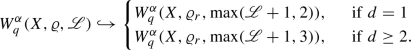  (4.2)

  Moreover, if $\Omega$ is bounded, or if $r=1$, or if ${\mathscr {L}}+1 \preceq {\mathscr {L}}$, then we further have

  

  (4.3)

• (2) If $\varrho \in {\mathtt {Spline}}^{r}({\mathbb {R}})$ is not a polynomial and $\Omega$ is bounded, then we have (with equivalent norms)

  

  (4.4)

• (3) For any $s \in {\mathbb {N}}$ we have

  

  (4.5)

The same results hold with instead of . $\blacktriangleleft$

Examples 3.15 and 3.16 provide important examples of depth growth functions ${\mathscr {L}}$ with ${\mathscr {L}}+1 \preceq {\mathscr {L}}$, so that (4.3) holds on any domain.

Remark 4.8

(Nestedness) For $1 \le r' \le r$, the function $\varrho := \varrho _{r'}$ is indeed a continuous piecewise polynomial with two pieces of degree at most r. Theorem 4.7 thus implies that if $\Omega$ is bounded or ${\mathscr {L}} + 1 \preceq {\mathscr {L}}$, then and .

We will see in Corollary 4.14 that if $2 {\mathscr {L}} \preceq {\mathscr {L}}$, then these embeddings are indeed equalities if $2 \le r' \le r$.$\blacklozenge$

The main idea behind the proof of Theorem 4.7 is to combine Lemma 2.19 and its consequences with the following results proved in Appendices C.1–C.2.

Lemma 4.9

Consider $\varrho :{\mathbb {R}}\rightarrow {\mathbb {R}}$ a continuous piecewise polynomial function with at most $n \in {\mathbb {N}}$ pieces of degree at most $r \in {\mathbb {N}}$. With³$w := 2 \cdot (4^{r}-1) / 3$ and $m := 2^{r} - 1$ we have

$$\begin{aligned} \varrho \in \overline{{\mathtt {NN}}^{\varrho _{r},1,1}_{4(r+1)+(n-1)w,2,2(r+1)+(n-1)m}}, \end{aligned}$$

where the closure is with respect to the topology of locally uniform convergence. For $r=1$ (that is, when $\varrho$ is continuous and piecewise affine with at most $n \in {\mathbb {N}}$ pieces and $\varrho _r = \varrho _1$), we even have ${\varrho \in {\mathtt {SNN}}^{\varrho _{r},1,1}_{2(n+1),2,n+1}}$.$\blacktriangleleft$

Lemma 4.10

Consider $r \in {\mathbb {N}}$ and $\varrho \in {\mathtt {Spline}}^{r} ({\mathbb {R}})$. If $\varrho$ is not a polynomial, then $\varrho _r \in \overline{{\mathtt {NN}}^{\varrho ,1,1}_{5^{r}r!,2,3^{r}r!}}$, where the closure is with respect to locally uniform convergence.$\blacktriangleleft$

For bounded $\Omega$, locally uniform convergence on ${\mathbb {R}}^{d}$ implies convergence in for all $p \in (0,\infty ]$. To similarly “upgrade” locally uniform convergence to convergence in X on unbounded domains, we use the following localization lemma which is proved in Appendix C.3.

Lemma 4.11

Consider $d,k \in {\mathbb {N}}$, $r \in {\mathbb {N}}_{\ge 2}$. There is $c = c(d,k,r) \in {\mathbb {N}}$ such that⁴ for any $W,L,N \in {\mathbb {N}}$, $g \in {\mathtt {NN}}^{\varrho _{r},d,k}_{W,L,N}$, $R \ge 1,\delta > 0$, there is $g_{R,\delta } \in {\mathtt {NN}}^{\varrho _{r},d,k}_{cW,\max \{ L+1, 3 \},cN}$, such that

$$\begin{aligned} |g_{R,\delta } ( x) - ({\mathbb {1}}_{[-R,R]^{d}} \cdot g)(x)| \le 2 \cdot |g(x)| \cdot {\mathbb {1}}_{[-R-\delta ,R+\delta ]^{d} {\setminus } [-R,R]^{d}} (x) \qquad \forall \, x \in {\mathbb {R}}^d .\nonumber \\ \end{aligned}$$

(4.6)

For $d=1$, the same holds with $\max \{ L+1,2 \}$ layers instead of $\max \{ L+1,3 \}$.$\blacktriangleleft$

The following proposition describes how one can “upgrade” the locally uniform convergence to convergence in , at the cost of slightly increasing the depth of the approximating networks.

Proposition 4.12

Consider $\Omega \subset {\mathbb {R}}^d$ an admissible domain and with $d,k \in {\mathbb {N}}$, $p \in (0,\infty ]$. Assume $\varrho \in \overline{{\mathtt {NN}}^{\varrho _{r},1,1}_{\infty ,2,m}}$ where the closure is with respect to locally uniform convergence and $r \in {\mathbb {N}}_{\ge 2}$, $m \in {\mathbb {N}}$. For any $W,N \in {\mathbb {N}}_{0} \cup \{\infty \}$, $L \in {\mathbb {N}}\cup \{\infty \}$, we have, with closure in X,

$$\begin{aligned} {\mathtt {NN}}_{W,L,N}^{\varrho ,d, k}(\Omega ) \cap X \subset \overline{ {\mathtt {NN}}^{\varrho _r, d, k}_{cWm^{2}, \max \{ L+1,3 \},cNm}(\Omega ) \cap X }^{X} , \end{aligned}$$

where $c = c(d,k, r) \in {\mathbb {N}}$ is as in Lemma 4.11. If $d=1$, the same holds with $\max \{ L+1,2 \}$ layers instead of $\max \{ L+1,3 \}$. If $\Omega$ is bounded, or if $\varrho \in {\mathtt {NN}}^{\varrho _{r},1,1}_{\infty ,2,m}$ with $r=1$, then the same holds with $c=1$ and L layers instead of $\max \{ L+1, 3 \}$ (resp. instead of $\max \{ L+1, 2 \}$ when $d=1$). $\blacktriangleleft$

The proof is in Appendix C.4. We are now equipped to prove Theorem 4.7.

Proof of Theorem 4.7

We give the proof for ; minor adaptations yield the results for .

For Claim (1), first note that Lemma 4.9 shows that there is some $m \in {\mathbb {N}}$ satisfying $\varrho \in \overline{{\mathtt {NN}}_{\infty ,2,m}^{\varrho _r,1,1}}$, where the closure is with respect to locally uniform convergence. Define $\ell := 3$ if $d \ge 2$ (resp. $\ell := 2$ if $d=1$) and $\widetilde{{\mathscr {L}}}:= \max \{ {\mathscr {L}}+1,\ell \}$ (resp. $\widetilde{{\mathscr {L}}}:= {\mathscr {L}}$ when $\Omega$ is bounded or $r=1$) and consider $c \in {\mathbb {N}}$ as in Proposition 4.12. Thus, since $\widetilde{{\mathscr {L}}}$ is non-decreasing, by Proposition 4.12 and Lemma 2.14, we have for all $n \in {\mathbb {N}}$

$$\begin{aligned} \mathtt {W}_n(X,\varrho ,{\mathscr {L}}) = {\mathtt {NN}}^{\varrho ,d,k}_{n,{\mathscr {L}}(n),\infty }(\Omega ) \cap X&\subset \overline{ {\mathtt {NN}}^{\varrho _r,d,k}_{cnm^{2},\widetilde{{\mathscr {L}}}(n),\infty }(\Omega ) \cap X }^{X} \\&\subset \overline{ {\mathtt {NN}}^{\varrho _r,d,k}_{cnm^{2},\widetilde{{\mathscr {L}}}(cnm^{2}),\infty }(\Omega ) \cap X }^{X}\\&= \overline{\mathtt {W}_{cm^{2}n}(X,\varrho _r, \widetilde{{\mathscr {L}}})}^{X}. \end{aligned}$$

Hence, for any $f \in X$ and $n \in {\mathbb {N}}$

$$\begin{aligned} E(f,\mathtt {W}_n(X,\varrho ,{\mathscr {L}}))_{X} \ge E\big ( f,\mathtt {W}_{cm^{2}n}(X,\varrho _r,\widetilde{{\mathscr {L}}})_{X} \big ) . \end{aligned}$$

Thus, Lemma 3.1 yields (4.2). When $\Omega$ is bounded or $r=1$, as $\widetilde{{\mathscr {L}}} = {\mathscr {L}}$, this yields (4.3). When ${\mathscr {L}}+1 \preceq {\mathscr {L}}$, as $\widetilde{{\mathscr {L}}} \le \max \{ {\mathscr {L}}+1,\ell \} \le {\mathscr {L}}+\ell +1$, we have $\widetilde{{\mathscr {L}}} \preceq {\mathscr {L}}+\ell +1 \preceq {\mathscr {L}}$ by Lemma 3.14, yielding again (4.3) by Lemma 3.12.

For Claim (2), if $\Omega$ is bounded and $\varrho \in {\mathtt {Spline}}^{r}({\mathbb {R}})$ is not a polynomial, combining Lemma 4.10 with Lemma 2.21, we similarly get the converse to  (4.3). This establishes (4.4).

We now prove Claim (3). Since $\varrho _{r^s} = \varrho _r \circ \cdots \circ \varrho _r$ (where $\varrho$ appears s times), Lemma 2.20 shows that ${\mathtt {NN}}^{\varrho _{r^{s}},d,k}_{W,L,N} \subset {\mathtt {NN}}^{\varrho _r,d,k}_{W+(s-1)N,1+s(L-1),sN}$ for all W, L, N. Combining this with Lemma 2.14, we obtain

$$\begin{aligned} {\mathtt {NN}}^{\varrho _{r^{s}},d,k}_{n,{\mathscr {L}}(n),\infty } \subset {\mathtt {NN}}^{\varrho _{r^{s}},d,k}_{n,{\mathscr {L}}(n),n} \subset {\mathtt {NN}}^{\varrho _r,d,k}_{sn,1+s({\mathscr {L}}(n)-1),sn} \subset {\mathtt {NN}}^{\varrho _r,d,k}_{sn,1+s({\mathscr {L}}(sn)-1),\infty } \quad \forall \, n \in {\mathbb {N}}. \end{aligned}$$

Therefore, we get for any $f \in X$ and $n \in {\mathbb {N}}$

$$\begin{aligned} E(f,\mathtt {W}_n(X,\varrho _{r^{s}},{\mathscr {L}}))_{X} \ge E\big ( f,\mathtt {W}_{sn}(X,\varrho _{r},1+s({\mathscr {L}}-1))_{X} \big ). \end{aligned}$$

Hence, we can finally apply Lemma 3.1 to obtain (4.5). $\square$

Remark 4.13

Inspecting the proofs, we see that if $\varrho \in {\mathtt {Spline}}^{r}$ has exactly one breakpoint, then $\varrho \in {\mathtt {NN}}^{\varrho _{r},1,1}_{w,2,m}$ and $\varrho _{r} \in {\mathtt {NN}}^{\varrho ,1,1}_{w,2,m}$ for some $w,m \in {\mathbb {N}}$. This is stronger than $\varrho \in \overline{{\mathtt {NN}}^{\varrho _{r},1,1}_{w,2,m}}$ (resp. than $\varrho _{r} \in \overline{{\mathtt {NN}}^{\varrho ,1,1}_{w,2,m}}$) and implies (4.4) with equivalent norms even on unbounded domains. Examples include the leaky ReLU [44], the parametric ReLU [33], and the absolute value which is used in scattering transforms [46].

Another spline of degree one is soft-thresholding, $\sigma (x) := x(1-\lambda /|x|)_{+}$, which appears in Iterative Shrinkage Thresholding Algorithms (ISTA) for $\ell ^{1}$ sparse recovery in the context of linear inverse problems [28, Chap. 3] and has been used in the Learned ISTA (LISTA) method [30]. As $\sigma \in {\mathtt {Spline}}^{1}$, using soft-thresholding as an activation function on bounded $\Omega$ is exactly as expressive as using the ReLU.$\blacklozenge$

4.2 Saturation Property of Approximation Spaces with Polynomial Depth Growth

For certain depth growth functions, the approximation spaces of $\varrho _{r}$-networks are independent of the choice of $r \ge 2$.

Corollary 4.14

With the notations of Theorem 4.7, if $2 {\mathscr {L}} \preceq {\mathscr {L}}$ then for every $r \in {\mathbb {N}}_{\ge 2}$ we have

(4.7)

(4.8)

where the equality is with equivalent quasi-norms.

Example 4.15

By Example 3.16, for polynomially growing depth we do have $2{\mathscr {L}} \preceq {\mathscr {L}}$. This includes the case ${\mathscr {L}}(n) = n+1$, which gives the same approximation spaces as ${\mathscr {L}} \equiv \infty$; see Remark 3.6.

In words, approximation spaces of $\varrho _{r}$-networks with appropriate depth growth have a saturation property: Increasing the degree r beyond $r=2$ does not pay off in terms of the considered function spaces. Note, however, that the constants in the norm equivalence may still play a qualitative role in practice.

Proof

We prove (4.7) the proof of (4.8) is similar. By Lemma 3.14, since $2{\mathscr {L}} \preceq {\mathscr {L}}$, we have $a {\mathscr {L}} + b \sim {\mathscr {L}}$ for all $a \ge 1$, $b \ge 1-a$. In particular, ${\mathscr {L}} + 1 \preceq {\mathscr {L}}$; hence, (4.3) holds with $\varrho = \varrho _{r'}$, $r' \in {\mathbb {N}}$, $1 \le r' \le r$. Combined with (4.5) and Lemma 3.12, since $r \le 2^r$ for $r \in {\mathbb {N}}$, we see

for all $r \in {\mathbb {N}}_{\ge 2}$. In the middle, we used that $1 + r ({\mathscr {L}} - 1) \preceq 1 + r {\mathscr {L}} \preceq (1 + r) {\mathscr {L}} \preceq {\mathscr {L}}$. $\square$

4.3 Piecewise Polynomial Activation Functions Yield Non-trivial Approximation Spaces

In light of the pathological example of Theorem 4.1, it is important to check that the approximation spaces and with $\varrho = \varrho _{r}$, $r \in {\mathbb {N}}$, are non-trivial: They are proper subspaces of . This is what we prove for any continuous and piecewise polynomial activation function $\varrho$.

Theorem 4.16

Let $\varrho : {\mathbb {R}}\rightarrow {\mathbb {R}}$ be continuous and piecewise polynomial (with finitely many pieces), let $\Omega \subset {\mathbb {R}}^d$ be measurable with non-empty interior, and let $s > 0$.

Let $p,q \in (0,\infty ]$, $k \in {\mathbb {N}}$, $\alpha \in (0,\infty )$, and . Finally, let ${\mathscr {L}}$ be a depth-growth function satisfying $\sup _{n\in {\mathbb {N}}} {\mathscr {L}}(n) \ge 2$. Then, and . $\blacktriangleleft$

The proof is given at the end of Appendix E.

4.4 ReLU Networks of Bounded Depth have Limited Expressiveness

In this subsection, we show that approximation spaces of ReLU networks of bounded depth and high approximation rate $\alpha$ are non-trivial in a very explicit sense: They fail to contain any nonzero function in $C_{c}^{3}({\mathbb {R}}^{d})$. This quite general obstruction to the expressiveness of shallow ReLU networks, and to the embedding of “classical” function spaces into the approximation spaces of shallow ReLU networks, is obtained by translating [55, Theorem 4.5] into the language of approximation spaces.

Theorem 4.17

Let $\Omega \subseteq {\mathbb {R}}^d$ be an open admissible domain, $p,q \in (0,\infty ]$, , $L \in {\mathbb {N}}$, and $\alpha > 0$.

• If , then $\lfloor L/2 \rfloor \ge \alpha / 2$;

• If , then $L - 1 \ge \alpha /2$. $\blacktriangleleft$

Before we give a proof, we immediately highlight a consequence.

Corollary 4.18

Let Y be a function space such that $C_c^3 (\Omega ) \cap Y \ne \{0\}$ where $\Omega \subseteq {\mathbb {R}}^d$ is an open admissible domain. For $p \in (0,\infty ]$, , $L \in {\mathbb {N}}$, $\alpha > 0$ and $q \in (0,\infty ]$, we have

• If , then $\lfloor L/2 \rfloor \ge \alpha /2$;

• If , then $L-1 \ge \alpha /2$. $\blacktriangleleft$

Remark

All “classical” function spaces (Sobolev, Besov, or modulation spaces, ...) include $C_c^\infty (\Omega )$; hence, this shows that none of these spaces embed into (resp. into ) for $\alpha > 2L$. In other words, to achieve embeddings into approximation spaces of ReLU networks with a good approximation rate, one needs depth! $\blacklozenge$

Proof of Theorem 4.17

The claimed estimates are trivially satisfied in case of $L = 1$; hence, we will assume $L \ge 2$ in what follows.

Let $f \in C_c^3 (\Omega )$ be not identically zero. We derive necessary criteria on L which have to be satisfied if or . By Eq. (3.2), we have and the same for ; thus, it suffices to consider the case $q = \infty$.

Extending f by zero outside $\Omega$, we can assume $f \in C_c^3({\mathbb {R}}^d)$ with ${{\text {supp}}}f \subset \Omega$. We claim that there is $x_0 \in {{\text {supp}}}(f) \subset \Omega$ with ${{\text {Hess}}}_f (x_0) \ne 0$, where ${{\text {Hess}}}_f$ denotes the Hessian of f. If this was false, we would have ${{\text {Hess}}}_f \equiv 0$ on all of ${\mathbb {R}}^d$, and hence, $\nabla f \equiv v$ for some $v \in {\mathbb {R}}^d$. This would imply $f (x) = \langle v, x \rangle + b$ for all $x \in {\mathbb {R}}^d$, with $b = f(0)$. However, since $f \equiv 0$ on the non-empty open set ${\mathbb {R}}^d {\setminus } {{\text {supp}}}(f)$, this would entail $v = 0$, and then, $f \equiv 0$, contradicting our choice of f.

Now, choose $r > 0$ such that $\Omega _0 := B_r (x_0) \subset \Omega$. Then, $f|_{\Omega _0}$ is not an affine-linear function, so that [55, Proposition C.5] yields a constant $C_1 = C_1(f,p) > 0$ satisfying

$$\begin{aligned} \Vert f - g \Vert _{L^p (\Omega _0)} \ge C_1 \cdot P^{-2} \quad \text {for each }P\text {-piecewise slice affine function }g : {\mathbb {R}}^d \rightarrow {\mathbb {R}}.\nonumber \\ \end{aligned}$$

(4.9)

Here, a function $g : {\mathbb {R}}^d \rightarrow {\mathbb {R}}$ is called P-piecewise slice affine if for arbitrary $x_0, v \in {\mathbb {R}}^d$ the function $g_{x_0, v} : {\mathbb {R}}\rightarrow {\mathbb {R}}, t \mapsto g(x_0 + t v)$ is piecewise affine-linear with at most P pieces; that is, $g_{x_0, v} \in {\mathtt {PPoly}}_{P}^1 ({\mathbb {R}})$.

Now, Lemma 5.19 (which will be proved independently) shows that there is a constant $K = K(L) \in {\mathbb {N}}$ such that

$$\begin{aligned} {\mathtt {NN}}_{W,L,\infty }^{\varrho _1, 1, 1} \subset {\mathtt {PPoly}}_{K \cdot W^{\lfloor L/2 \rfloor }}^1 ({\mathbb {R}}) \qquad \text {and} \qquad {\mathtt {NN}}_{\infty ,L,N}^{\varrho _1, 1, 1} \subset {\mathtt {PPoly}}_{K \cdot N^{L-1}}^1 ({\mathbb {R}}) \end{aligned}$$

for all $N \in {\mathbb {N}}$. Furthermore, if $g \in {\mathtt {NN}}_{W,L,N}^{\varrho _1,d,1}$, then Lemma 2.18 shows $g_{x_0, v} \in {\mathtt {NN}}_{W,L,N}^{\varrho _1,1,1}$; here, we used that the affine map $T : {\mathbb {R}}\rightarrow {\mathbb {R}}^d , t \mapsto x_0 + t v$ satisfies $\Vert T \Vert _{\ell ^{0,\infty }_*} \le 1$. In combination, we see that each $g \in {\mathtt {NN}}_{W,L,\infty }^{\varrho _1,d,1}$ is P-piecewise slice affine with $P = K \cdot W^{\lfloor L/2 \rfloor }$, and each $g \in {\mathtt {NN}}_{\infty ,L,N}^{\varrho _1,d,1}$ is P-piecewise slice affine with $P = K \cdot N^{L-1}$.

Now, if , then there is a constant $C_2 = C_2(f,\alpha ,p) > 0$ such that for each $n \in {\mathbb {N}}$, there is $g_n \in {\mathtt {NN}}_{n,L,\infty }^{\varrho _1,d,1}$ satisfying $\Vert f - g_n \Vert _{L^p(\Omega _0)} \le \Vert f - g_n \Vert _{X} \le C_2 \cdot n^{-\alpha }$. Furthermore, since $g_n$ is P-piecewise slice affine with $P = K \cdot n^{\lfloor L/2 \rfloor }$, Eq. (4.9) shows that $K^{-2} C_1 \cdot n^{-2 \lfloor L/2 \rfloor } \le \Vert f - g_n \Vert _{L^p(\Omega _0)} \le C_2 \cdot n^{-\alpha }$. Since this holds for all $n \in {\mathbb {N}}$, we get $\alpha - 2 \lfloor L/2 \rfloor \le 0$, as claimed.

The proof in case of is almost identical, and hence omitted. $\square$

Our next result shows that for networks of fixed depth, neural networks using the activation function $\varrho _r$ with $r \ge 2$ are strictly more expressive than ReLU networks—at least in the regime of very high approximation rates.

Corollary 4.19

Consider $\Omega \subseteq {\mathbb {R}}^d$ an open admissible domain, $p \in (0,\infty ]$, , $L \in {\mathbb {N}}$. In case of $d = 1$, assume that $r \ge 4$ and $L \ge 2$, or that $r \in \{2,3\}$ and $L \ge 3$. In case of $d > 1$, assume instead that $r \ge 4$ and $L \ge 3$, or that $r \in \{2,3\}$ and $L \ge 5$. Then, the following hold:

Proof

We use Lemma 4.20 to get and , and we conclude using Corollary 4.18. $\square$

Lemma 4.20

Consider $d,r,L \in {\mathbb {N}}$, $\Omega \subset {\mathbb {R}}^d$ an open admissible domain, $p \in (0,\infty ]$, . In case of $d = 1$, assume that $r \ge 4$ and $L \ge 2$, or that $r \in \{2,3\}$ and $L \ge 3$. In case of $d > 1$, assume instead that $r \ge 4$ and $L \ge 3$, or that $r \in \{2,3\}$ and $L \ge 5$.

Then, for each $\alpha > 0$ and $q \in (0,\infty ]$, we have $\blacktriangleleft$

Proof

Since $\Omega$ is an admissible domain, it is non-empty. Being open, $\Omega$ thus contains a hyper-rectangle $[a,b] := \prod _{i=1}^d [a_i,b_i] \subset \Omega$, where $a_i < b_i$.

For $r' \ge 2$, let $\sigma _{r'} \in {\mathtt {SNN}}^{\varrho _{r'},1,1}_{2(r'+1),2,r'+1}$ be the function constructed in Lemma 4.4. As $\sigma _{r'}$ satisfies (3.9), the function g built from $\sigma _{r'}$ in Lemma 3.26-(2) for small enough $\varepsilon$ is nonzero and satisfies ${{{\text {supp}}}(g) \subset [a,b] \subset \Omega }$ and $g \in {\mathtt {NN}}_{\infty ,3,\infty }^{\varrho _{r'},d,1}$ (resp. $g \in {\mathtt {NN}}_{\infty ,2,\infty }^{\varrho _{r'},d,1}$ when $d=1$). Note that if $r' \ge 4$, then $\varrho _{r'} \in C^{3}({\mathbb {R}})$; hence, $g \in C^{3}_{c}({\mathbb {R}}^{d}) {\setminus } \{0\}$.

When $r \ge 4$, set $r':=r$ so that $g \in {\mathtt {NN}}^{\varrho _{r},d,1}_{\infty ,3,\infty }$ ($g \in {\mathtt {NN}}^{\varrho _{r},d,1}_{\infty ,2,\infty }$ when $d=1$). When $r \in \{2,3\}$, set $r' := r^{2} \ge 4$. As $\varrho _{r'} = \varrho _{r} \circ \varrho _{r}$, Lemma 2.20 with $s=2$ yields $g \in {\mathtt {NN}}^{\varrho _{r},d,1}_{\infty ,5,\infty }$ ($g \in {\mathtt {NN}}^{\varrho _{r},d,1}_{\infty ,3,\infty }$ for $d=1$).

It is not hard to see that our assumptions regarding L imply in each case for n large enough that $g|_{\Omega } \in \mathtt {W}_{n}(X,\varrho _{r},L) \cap \mathtt {N}_{n}(X,\varrho _{r},L)$, and hence, . $\square$

5 Direct and Inverse Estimates with Besov Spaces

In this section, we characterize certain embeddings

• of Besov spaces into and ; these are called direct estimates;

• of and into Besov spaces; these are called inverse estimates.

Since the approximation classes for output dimension $k > 1$ are k-fold Cartesian products of the classes for $k=1$ (cf. Remark 3.17), we focus on scalar output dimension $k=1$. We will use so-called Jackson inequalities and Bernstein inequalities, as well as the notion of real interpolation spaces. These concepts are recalled in Sect. 5.1, while Besov spaces and some of their properties are briefly recalled in Sect. 5.2 before we proceed to our main results.

5.1 Reminders on Interpolation Theory

Given two quasi-normed vector spaces $(Y_J, \Vert \cdot \Vert _{Y_J})$ and $(Y_B, \Vert \cdot \Vert _{Y_B})$ with $Y_J \hookrightarrow X$ and $Y_B \hookrightarrow X$ for a given quasi-normed linear space $(X, \Vert \cdot \Vert _X)$, we say that $Y_J$ fulfills a Jackson inequality with exponent $\gamma > 0$ with respect to the family $\Sigma = (\Sigma _n)_{n \in {\mathbb {N}}_0}$, if there is a constant $C_J > 0$ such that

$$\begin{aligned} E(f,\Sigma _{n})_{X} \le C_J \cdot n^{-\gamma } \cdot \Vert f \Vert _{Y_J} \qquad \forall \, f \in Y_J \text { and } n \in {\mathbb {N}}. \end{aligned}$$

(J)

We say that $Y_B$ fulfills a Bernstein inequality with exponent $\gamma > 0$ with respect to $\Sigma = (\Sigma _n)_{n \in {\mathbb {N}}_0}$, if there is a constant $C_B > 0$ such that

$$\begin{aligned} \Vert \varphi \Vert _{Y_B} \le C_B \cdot n^\gamma \cdot \Vert \varphi \Vert _X \qquad \forall \, n \in {\mathbb {N}}\text { and } \varphi \in \Sigma _n . \end{aligned}$$

(B)

As shown in the proof of [21, Chapter 7, Theorem 9.1], we have the following:

Proposition 5.1

Denote by $(X,Y)_{\theta , q}$ the real interpolation space obtained from X, Y, as defined, e.g., in [21, Chapter 6, Section 7]. Then, the following hold:

• If $Y_J \hookrightarrow X$ fulfills the Jackson inequality with exponent $\gamma > 0$, then

  

• If $Y_B \hookrightarrow X$ fulfills the Bernstein inequality with exponent $\gamma >0$, then

  

In particular, if the single space $Y = Y_J = Y_B$ satisfies both inequalities with the same exponent $\gamma$, then for all $0< \alpha < \gamma$ and $0 < q \le \infty$.

By [21, Chapter 7, Theorem 9.3], if $\Sigma$ satisfies Properties (P1)–(P5), then for $0 < \tau \le \infty$, $0< \alpha < \infty$ the space $Y := A^{\alpha }_{\tau }(X,\Sigma )$ satisfies matching Jackson and Bernstein inequalities with exponent $\gamma :=\alpha$. The Bernstein inequality reads

$$\begin{aligned} \exists \, C = C (\alpha ,\tau ,X) > 0 \quad \forall \, n \in {\mathbb {N}}\text { and } \varphi \in \Sigma _n : \quad \Vert \varphi \Vert _{A^{\alpha }_{\tau }(X,\Sigma )} \le C \cdot n^\alpha \cdot \Vert \varphi \Vert _X .\nonumber \\ \end{aligned}$$

(5.1)

We will also use the following well-known property of (real) interpolation spaces (see [21, Chapter 6, Theorem 7.1]): For quasi-Banach spaces $X_1, X_2$ and $Y_1, Y_2$, assume that $T : X_1 + X_2 \rightarrow Y_1 + Y_2$ is linear and such that $T|_{X_i} : X_i \rightarrow Y_i$ is bounded for $i \in \{1,2\}$. Then, $T|_{(X_1, X_2)_{\theta ,q}} : (X_1, X_2)_{\theta ,q} \rightarrow (Y_1, Y_2)_{\theta ,q}$ is well defined and bounded for all $\theta \in (0,1)$ and $q \in (0,\infty ]$.

5.2 Reminders on Besov Spaces

We refer to [20, Section 2] for the definition of the Besov spaces $B^{s}_{\sigma ,\tau } (\Omega ) := B^s_{\tau }(X_\sigma (\Omega ;{\mathbb {R}}))$ with $\sigma , \tau \in (0,\infty ]$, $s \in (0,\infty )$ and with a Lipschitz domain⁵$\Omega \subset {\mathbb {R}}^{d}$ (see [1, Definition 4.9] for the precise definition of these domains).

As shown in [19, Theorem 7.1], we have for all $p, s \in (0,\infty )$ the embedding

$$\begin{aligned} B^{s}_{\sigma ,p}( (0,1)^d ) \hookrightarrow L_p( (0,1)^d ;{\mathbb {R}}), \quad \text {provided} \quad \sigma = (s/d + 1/p)^{-1}. \end{aligned}$$

Combined with the embedding $B^{s}_{p,q}(\Omega ) \hookrightarrow B^s_{p,q'}(\Omega )$ for $q \le q'$ (see [17, Displayed equation on Page 92]) and because of $\sigma = (s/d + 1/p)^{-1} \le p$, we see that

$$\begin{aligned} B^{s}_{\sigma ,\sigma } ( (0,1)^d ) \hookrightarrow B^{s}_{\sigma ,p}( (0,1)^d ) \hookrightarrow L_p( (0,1)^d ;{\mathbb {R}}), \quad \text {provided} \quad \sigma = (s/d + 1/p)^{-1}. \nonumber \\ \end{aligned}$$

(5.2)

For the special case $\Omega = (0,1) \subset {\mathbb {R}}$ and each fixed $p \in (0,\infty )$, the sub-family of Besov spaces $B^{s}_{\sigma ,\sigma }( (0,1) )$ with $\sigma = (s/d+1/p)^{-1}$ satisfies

$$\begin{aligned} \big ( L_p( (0,1);{\mathbb {R}}), B^s_{\sigma , \sigma }( (0,1) ) \big )_{\theta ,q} = B^{\theta s}_{q,q}( (0,1) ), \quad \text {for}\ 0< \theta < 1, \text {where}\ q= (\theta s + 1/p)^{-1}.\nonumber \\ \end{aligned}$$

(5.3)

This is shown in [21, Chapter 12, Corollary 8.5].

Finally, from the definition of Besov spaces given in [20, Equation (2.2)] it is clear that

$$\begin{aligned} B_{p,q}^\alpha (\Omega ) \hookrightarrow B_{p,q}^\beta (\Omega ) \quad \text {if} \quad p,q \in (0,\infty ] \text { and } 0< \beta < \alpha . \end{aligned}$$

(5.4)

5.3 Direct Estimates

In this subsection, we investigate embeddings of Besov spaces into the approximation spaces where $\Omega \subseteq {\mathbb {R}}^{d}$ is an admissible domain and with $p \in (0,\infty ]$. For technical reasons, we further assume $\Omega$ to be a bounded Lipschitz domain, such as $\Omega =(0,1)^d$, see [1, Definition 4.9]. The main idea is to exploit known direct estimates for Besov spaces on such domains which give error bounds for the n-term approximations with B-spline-based wavelet systems, see [19].

For $t \in {\mathbb {N}}_0$ and $d \in {\mathbb {N}}$, the tensor product B-spline is $\beta _d^{(t)} (x_1,\dots ,x_d) := \beta _{+}^{(t)}(x_1) \, \beta _{+}^{(t)}(x_2) \, \cdots \beta _{+}^{(t)}(x_d),$ where $\beta _+^{(t)}$ is as introduced in Definition 4.5. Notice that $\beta _d^{(0)} = {\mathbb {1}}_{[0,1)^{d}}$.

By Lemma 4.4, there is ${\sigma _{r}} \in {\mathtt {NN}}^{\varrho _{r},1,1}_{2(r+1),2,r+1}$ satisfying (3.9); hence, by Lemma 3.26 there is $L \le 3$ such that for $\varepsilon > 0$, we can approximate $\beta _d^{(0)}$ with $g_\varepsilon = {\mathtt {R}}(\Phi _\varepsilon )$ with precision $\Vert \beta _d^{(0)} - g_\varepsilon \Vert _{L_p({\mathbb {R}}^d)} < \varepsilon$, where $L(\Phi _\varepsilon ) = L$ and $\Phi _\varepsilon \in {\mathtt {NN}}^{\varrho _{r},d,1}_{w,3,m}$, for suitable $w = w(d,r), m = m(d,r) \in {\mathbb {N}}$. Furthermore, if $d = 1$, then Lemma 3.26 shows that the same holds for some $\Phi _\varepsilon \in {\mathtt {NN}}^{\varrho _r,d,1}_{w,2,m}$.

For approximating $\beta ^{(t)}_d$ (with $t \in {\mathbb {N}}$) instead of $\beta _d^{(0)}$, we can actually do better. In fact, we prove in Appendix D.1 that one can implement $\beta _d^{(t)}$ as a $\varrho _{t}$-network, provided that $t \ge \min \{ d,2 \}$.

Lemma 5.2

Let $d,t \in {\mathbb {N}}$ with $t \ge \min \{ d, 2 \}$. Then, the tensor product B-spline

$$\begin{aligned} \beta _d^{(t)} : {\mathbb {R}}^d \rightarrow {\mathbb {R}}, \quad \beta _d^{(t)} (x) := \beta _{+}^{(t)}(x_1) \beta _{+}^{(t)}(x_2) \cdots \beta _{+}^{(t)} (x_d) \end{aligned}$$

(5.5)

satisfies $\beta _d^{(t)} \in {\mathtt {NN}}^{\varrho _t,d,1}_{w,L,m}$ with $L = 2 + 2 \lceil \log _{2}d\rceil$ and

$$\begin{aligned} {\left\{ \begin{array}{ll} w = 28 d(t+1) \;{\mathrm{and}}\; m = 13d(t+1), &{}\quad {\mathrm{if}}\; d > 1, \\ w = 2 (t+2) \;{\mathrm{and}}\; m = t+2 , &{} \quad {\mathrm{if}}\; d = 1. \end{array}\right. } \blacktriangleleft \end{aligned}$$

In the following, we will consider n-term approximations with respect to the continuous wavelet-type system generated by $\beta _d^{(t)}$. Precisely, for $a > 0$ and $b \in {\mathbb {R}}^d$, define $\beta ^{(t)}_{a,b} := \beta _d^{(t)} (a \cdot + b)$. The continuous wavelet-type system generated by $\beta _d^{(t)}$ is then ${\mathcal {D}}_d^{t} := \{ \beta ^{(t)}_{a,b} :a \in (0,\infty ), b \in {\mathbb {R}}^d \}$. For any $t \in {\mathbb {N}}_{0}$, we define $\Sigma _{0}({\mathcal {D}}_d^t) := \{0\}$, and the reservoir of all n-term expansions from ${\mathcal {D}}_d^{t}$, $n \in {\mathbb {N}}$, is given by

$$\begin{aligned} \Sigma _n({\mathcal {D}}_d^{t}) := \bigg \{ g = \sum _{i=1}^n c_i g_i :c_i \in {\mathbb {R}}, g_i \in {\mathcal {D}}_d^t \bigg \}. \end{aligned}$$

The following lemma relates $\Sigma _n({\mathcal {D}}_d^{t})$ to ${\mathtt {NN}}^{\varrho _{r},d,1}_{cn,L,cn}$ for a suitably chosen constant $c=c(d,r,t) \in {\mathbb {N}}$.

Lemma 5.3

Consider $d \in {\mathbb {N}}$, $t \in {\mathbb {N}}_{0}$, $p \in (0,\infty ]$, .

• (1) If $t=0$ and $p<\infty$, then, with $L := \min \{ d+1,3 \}$ and $c = c(d,r) \in {\mathbb {N}}$, we have

  $$\begin{aligned} \Sigma _{n}({\mathcal {D}}_d^0) \subset \overline{{\mathtt {NN}}^{\varrho _{r},d,1}_{cn,L,cn} \cap X}^{X} \qquad \forall \, n,r \in {\mathbb {N}}. \end{aligned}$$

  (5.6)

• (2) If $t \ge \min \{ d,2 \}$, then, with $L := 2 + 2 \lceil \log _{2} d \rceil$, we have for any $p \in (0,\infty ]$ that

  $$\begin{aligned} \Sigma _n({\mathcal {D}}_d^t) \subset {\mathtt {NN}}^{\varrho _t,d,1}_{cn,L,cn} \cap X \qquad \forall \, n \in {\mathbb {N}}, \end{aligned}$$

  (5.7)

  where $c = c(d,t) \in {\mathbb {N}}$. $\blacktriangleleft$

Proof

Part (1): For $t = 0$, $r \in {\mathbb {N}}$, $0< p < \infty$, we have already noticed before Lemma 5.2 that there exist $w = w(d,r), m = m(d,r) \in {\mathbb {N}}$ such that $\beta _d^{(0)} \in \overline{{\mathtt {NN}}^{\varrho _r,d,1}_{w,L,m} \cap X}^{X}$, where $L = \min \{ d+1,3 \}$. Since $\beta _{a,b}^{(0)} = \beta _d^{(0)} \circ P_{a,b}$ for the affine map $P_{a,b} : {\mathbb {R}}^d \rightarrow {\mathbb {R}}^d, x \mapsto a x + b$ and since $\Vert P_{a,b}\Vert _{\ell ^{0,\infty }_*} = 1$, Lemmas 2.17-(1) and 2.18-(1) yield $\beta _{a,b}^{(0)} \in \overline{{\mathtt {NN}}^{\varrho _r,d,1}_{c,L,c} \cap X}^{X}$ with $c := \max \{ w,m \}$. Thus, the claim follows from Parts (1) and (3) of Lemma 2.17.

Part (2): For $t \ge \min \{ d,2 \}$, Lemma 5.2 shows that $\beta _{a,b}^{(t)} \in {\mathtt {NN}}^{\varrho _t,d,1}_{c,L,c} \cap X$ with $L = 2 + 2 \lceil \log _2 d \rceil$ and $c := \max \{ w,m \}$ where $w = w(d,t)$ and $m = m(d,t)$ are as in Lemma 5.2. As before, we conclude using Parts (1) and (3) of Lemma 2.17. $\square$

Corollary 5.4

Consider $d \in {\mathbb {N}}$, $\Omega \subset {\mathbb {R}}^{d}$ an admissible domain, $p \in (0, \infty ]$, , ${\mathscr {L}}$ a depth growth function, $L := \sup _{n} {\mathscr {L}}(n) \in {\mathbb {N}}\cup \{\infty \}$. For $t \in {\mathbb {N}}_{0}$, define $\Sigma ({\mathcal {D}}_d^{t}) := ( \Sigma _{n}({\mathcal {D}}_d^t))_{n \in {\mathbb {N}}_{0}}$.

• (1) If $L \ge \min \{ d+1, 3 \}$ and $p < \infty$, then for any $r \ge 1$

  

• (2) If $L \ge 2 + 2 \lceil \log _{2} d\rceil$ then for any $r \ge \min \{ d,2 \}$, we have

  

Proof

For the proof of Part (1) let $L_0 := \min \{d+1, 3\}$, while $L_0 := 2 + 2 \lceil \log _2 d \rceil$ for the proof of Part (2). Since $L \ge L_0$, there is $n_{0} \in {\mathbb {N}}$ such that ${\mathscr {L}}(n) \ge L_0$ for all $n \ge n_{0}$.

We first start with the proof of Part (2). By Lemma 5.3-(2), with $t = r \ge \min \{ d,2 \}$, Eq. (5.7) holds for some $c \in {\mathbb {N}}$. For $n \ge n_{0}/c$, we have $2 + 2 \lceil \log _2 d \rceil = L_0 \le {\mathscr {L}}(cn)$, whence

$$\begin{aligned} \Sigma _n({\mathcal {D}}_d^t) \subset \overline{\mathtt {W}_{cn}(X,\varrho _{r},{\mathscr {L}})}^{X}. \end{aligned}$$

Therefore, we see that

$$\begin{aligned} E(f,\Sigma _n({\mathcal {D}}_d^t))_{X} \ge E(f,\mathtt {W}_{cn}(X,\varrho _{r},{\mathscr {L}}))_{X} \quad \forall \, f \in X \text { and } n \ge \tfrac{n_0}{c}. \end{aligned}$$

(5.8)

For the proof of Part (1), the same reasoning with (5.6) instead of (5.7) yields (5.8) with $t=0$ and any $r \in {\mathbb {N}}$. For both parts, we conclude using Lemma 3.1 and the associated remark. $\square$

Theorem 5.5

Let $\Omega \subset {\mathbb {R}}^{d}$ be a bounded Lipschitz domain of positive measure. For $p \in (0,\infty ]$, define $X_p (\Omega )$ as in Eq. (1.3). Let ${\mathscr {L}}$ be a depth growth function.

• (1) Suppose that $d = 1$ and $L := \sup _{n \in {\mathbb {N}}} {\mathscr {L}}(n) \ge 2$. Then, the following holds for each $r \in {\mathbb {N}}$:

  

  (5.9)

• (2) Suppose that $d > 1$ and $L := \sup _{n \in {\mathbb {N}}} {\mathscr {L}}(n) \ge 3$, and let $r \in {\mathbb {N}}$.

  Define $r_0 := r$ if $r \ge 2$ and $L \ge 2 + 2 \lceil \log _2 d \rceil$, and $r_0 := 0$ otherwise.

  Then,

  

  (5.10)

Remark 5.6

If $\Omega$ is open, then each Besov space $B_{p,q}^{s d}(\Omega )$ contains $C_{c}^{3}(\Omega )$. Hence, by Corollary 4.18, the embeddings (5.9) or (5.10) with $r = 1$ imply that $\lfloor L/2 \rfloor \ge s / 2$. This is indeed the case, since these embeddings for $r = 1$ are only established when $L \ge 2$ and $0< d s < 1 + \min \{ p^{-1},1 \} \le 2$, which implies $s / 2 < 1/d \le 1 \le \lfloor L/2 \rfloor$.$\blacklozenge$

Proof of Theorem 5.5

See Appendix D.2. $\square$

5.4 Limits on Possible Inverse Estimates

For networks of finite depth ${\mathscr {L}} \equiv L < \infty$, there are limits on possible embeddings of (resp. of ) into Besov spaces.

Theorem 5.7

Consider $\Omega = (0,1)^{d}$, $p \in (0,\infty ]$, , ${\mathscr {L}}$ a depth growth function such that $L := \sup _{n} {\mathscr {L}}(n) \in {\mathbb {N}}_{\ge 2} \cup \{\infty \}$ and $r \in {\mathbb {N}}$. For $\sigma , \tau , q \in (0,\infty ]$ and $\alpha , s \in (0,\infty )$, the following claims hold⁶:

• (1) If , then $\alpha \ge \lfloor L/2\rfloor \cdot \min \{ s, 2 \}$.

• (2) If , then $\alpha \ge (L-1) \cdot \min \{ s, 2 \}$. $\blacktriangleleft$

A direct consequence is that for networks of unbounded depth ($L=\infty$), none of the spaces , embed into any Besov space of strictly positive smoothness $s>0$.

Remark 5.8

For $L=2$, as $\lfloor L/2\rfloor = L-1$, the two inequalities resulting from Theorem 5.7 match. This is natural as for $L=2$ we know from Lemma 3.9 that . For $L \ge 3$, the inequalities no longer match. Each inequality is in fact stronger than what would be achieved by simply combining the other one with Lemma 3.9. Note also that in contrast to the direct estimate (5.10) of Theorem 5.5 where the Besov spaces are of smoothness sd, here the dimension d does not appear. $\blacklozenge$

The proof of Theorem 5.7 employs a particular family of oscillating functions that have a long history [31] in the analysis of neural networks and of the benefits of depth [64].

Fig. 4

A plot of the function $\Delta _j$ (for $j = 3$)

Definition 5.9

(Sawtooth functions) Consider $\beta _{+}^{(1)}$ the B-spline of degree one, and $\Delta _{1} := \beta _{+}^{(1)}(2\cdot )$ the “hat” function supported on [0, 1]. For $j \ge 1$, the univariate “sawtooth” function of order j,

$$\begin{aligned} \Delta _{j} = \sum _{k=0}^{2^{j-1}-1} \Delta _{1}(2^{j-1}\cdot -k), \end{aligned}$$

(5.11)

has support in [0, 1] and is made of $2^{j-1}$ triangular “teeth” (see Fig. 4). The multivariate sawtooth function $\Delta _{j,d}$ is defined as $\Delta _{j,d}(x) := \Delta _{j}(x_{1})$ for $x = (x_{1},\ldots ,x_{d}) \in {\mathbb {R}}^{d}$, $j \in {\mathbb {N}}$. $\blacktriangleleft$

An important property of $\Delta _j$ is that it is a realization of a $\varrho _1$-network of specific complexity. The proof of this lemma is in Appendix D.3.

Lemma 5.10

Let $L \in {\mathbb {N}}_{\ge 2}$ and define $C_L := 4 \, L + 2^{L-1}$. Then,

$$\begin{aligned} \Delta _j \in {\mathtt {NN}}^{\varrho _1, 1, 1}_{\infty , L, C_L \cdot 2^{j / (L-1)}} \qquad \text {and} \qquad \Delta _j \in {\mathtt {NN}}^{\varrho _1, 1, 1}_{C_L \cdot 2^{j / \lfloor L/2 \rfloor }, L, \infty } \qquad \forall \, j \in {\mathbb {N}}. \blacktriangleleft \end{aligned}$$

Corollary 5.11

For $L \in {\mathbb {N}}_{\ge 2}$, let $C_L$ as in Lemma 5.10. Then,

$$\begin{aligned} \Delta _{j,d} \in {\mathtt {NN}}^{\varrho _1, d, 1}_{\infty , L, C_L \cdot 2^{j / (L-1)}} \qquad \text {and} \qquad \Delta _{j,d} \in {\mathtt {NN}}^{\varrho _1, d, 1}_{C_L \cdot 2^{j / \lfloor L/2 \rfloor }, L, \infty } \qquad \forall \, j \in {\mathbb {N}}. \blacktriangleleft \end{aligned}$$

Proof

We have $\Delta _{j,d} = \Delta _j \circ T$ for the affine map $T : {\mathbb {R}}^d \rightarrow {\mathbb {R}}, (x_1,\dots ,x_d) \mapsto x_1$, which satisfies $\Vert T\Vert _{\ell ^{0,\infty }_*} = 1$. Now, the claim is a direct consequence of Lemmas 5.10 and 2.18-(1). $\square$

We further prove in Appendix D.4 that the Besov norm of $\Delta _{j,d}$ grows exponentially with j:

Lemma 5.12

Let $d \in {\mathbb {N}}$ and $\Omega = (0,1)^d$. Let $p,q \in (0,\infty ]$ and $s \in (0, \infty )$ be arbitrary. Let ${s'} \in (0,2)$ with ${s'} \le s$. There is a constant $c = c(d,p,q,s,{s'}) > 0$ such that

$$\begin{aligned} \Vert \Delta _{j,d}\Vert _{B^s_{p,q} (\Omega )} \ge c \cdot 2^{{s'} j} \qquad \forall \, j \in {\mathbb {N}}. \blacktriangleleft \end{aligned}$$

Given this lower bound on the Besov space norm of the sawtooth function $\Delta _{j,d}$, we can now prove the limitations regarding possible inverse estimates that we announced above.

Proof of Theorem 5.7

We start with the proof for . Let us fix $\ell \in {\mathbb {N}}$ with $\ell \le \lfloor L/2 \rfloor$, and note that $2\ell \le L$, so that there is some $j_0 = j_0 (\ell , {\mathscr {L}}) \in {\mathbb {N}}$ such that ${\mathscr {L}}(2^j) \ge 2\ell$ for all ${j \ge j_0}$. Now, Corollary 5.11 (applied with $2\ell$ instead of L) shows that $\Delta _{\ell j, d} \in {\mathtt {NN}}^{\varrho _1, d, 1}_{C_{2\ell } 2^{(\ell j)/\ell }, 2\ell , \infty } \subset {\mathtt {NN}}^{\varrho _1, d, 1}_{C_{2\ell } 2^{j}, {\mathscr {L}}(C_{2\ell } 2^{j}), \infty }$ for all $j \ge j_0$ and a suitable constant $C_{2\ell } \in {\mathbb {N}}$. Therefore, the Bernstein inequality (5.1) yields a constant $C = C(d,\alpha , q, p) > 0$ such that

Let $s_0 := \min \{ 2, s \}$, let $0< s' < s_0$ be arbitrary, and note as a consequence of Eq. (4.3) that

Here, we used that $\Omega$ is bounded, so that Eq. (4.3) is applicable. Overall, as a consequence of this embedding and of Lemma 5.12, we obtain $c = c(d,s',s,\sigma ,\tau ) > 0$ and ${C' = C'(\sigma ,\tau ,s,p,q,\alpha ,{\mathscr {L}},\Omega ) > 0}$ satisfying

for all $j \ge j_0$. This implies $s' \cdot \ell \le \alpha$. Since this holds for all $s' \in (0,s_0)$ and all $\ell \in {\mathbb {N}}$ with $\ell \le \lfloor L/2 \rfloor$, we get $\lfloor L/2 \rfloor \cdot s_0 \le \alpha$, as claimed.

Now, we prove the claim for . In this case, fix $\ell \in {\mathbb {N}}$ with $\ell +1 \le L$, and note that there is some $j_0 \in {\mathbb {N}}$ satisfying ${\mathscr {L}}(2^j) \ge \ell + 1$ for all $j \ge j_0$. Now, Corollary 5.11 (applied with $\ell +1$ instead of L) yields a constant $C_{\ell +1} \in {\mathbb {N}}$ such that $\Delta _{\ell j, d} \in {\mathtt {NN}}^{\varrho _1, d, 1}_{\infty , \ell +1, C_{\ell +1} 2^{(\ell j)/((\ell +1) - 1)}} \subset {\mathtt {NN}}^{\varrho _1, d, 1}_{\infty , {\mathscr {L}}(C_{\ell +1} 2^{j}), C_{\ell +1} 2^{j}}$ for all $j \ge j_0$. As above, the Bernstein inequality (5.1) therefore shows for all $j \ge j_0$ and some constant $C = C(d,\alpha ,q,p) < \infty$. Reasoning as above, we get that

for all $j \ge j_0$ and $0< s' < s_0 = \min \{2,s\}$. Therefore, $s' \cdot \ell \le \alpha$. Since this holds for all $s' \in (0,s_0)$ and all $\ell \in {\mathbb {N}}$ with $\ell + 1 \le L$, we get $\alpha \ge s_0 \cdot (L-1)$, as claimed. $\square$

5.5 Univariate Inverse Estimates ($d=1$)

The “no-go theorem” (Theorem 5.7) holds for $\Omega = (0,1)^{d}$ in any dimension $d \ge 1$, for any $0 < p \le \infty$. In this subsection, we show in dimension $d = 1$ that Theorem 5.7 is quite sharp. Precisely, we prove the following:

Theorem 5.13

Let $X = L_p(\Omega )$ with $\Omega =(0,1)$ and $p \in (0,\infty )$, let $r \in {\mathbb {N}}$, and let ${\mathscr {L}}$ be a depth growth function. Assume that $L := \sup _{n} {\mathscr {L}}(n) < \infty$. Setting $\nu := \lfloor L/2\rfloor$, the following statements hold:

• (1) For $s \in (0,\infty )$, $\alpha \in (0, \nu s)$ and $q \in (0,\infty ]$, we have

  

• (2) For $\alpha \in (0,\infty )$, we have

  

The same holds for instead of if we set $\nu := L-1$. $\blacktriangleleft$

The proof involves a Bernstein inequality for piecewise polynomials by Petrushev [56], and new bounds on the number of pieces of piecewise polynomials implemented by $\varrho _{r}$-networks. Petrushev considers the (nonlinear) set $\tilde{\mathtt {S}}(k,n)$ of all piecewise polynomials on (0, 1) of degree at most $r=k-1$ ($k \in {\mathbb {N}}$) with at most $n-1$ breakpoints in [0, 1]. In the language of Definition 4.6, $\tilde{\mathtt {S}}(k,n) = {\mathtt {PPoly}}_n^r ( (0,1) )$ is the set of piecewise polynomials of degree at most $r=k-1 \in {\mathbb {N}}_{0}$ with at most n pieces on (0, 1).

By [21, Chapter 12, Theorem 8.2] (see [56, Theorem 2.2] for the original proof), the following Bernstein-type inequality holds for each family $\Sigma := (\tilde{\mathtt {S}}(k,n))_{n \in {\mathbb {N}}}$, $k \in {\mathbb {N}}$:

Theorem 5.14

([56, Theorem 2.2]) Let $\Omega = (0,1)$, $p \in (0,\infty )$, $r \in {\mathbb {N}}_{0}$, and $s \in (0,r+1)$ be arbitrary, and set $\sigma := (s + 1/p)^{-1}$. Then, there is a constant $C < \infty$ such that we have

$$\begin{aligned} \Vert f \Vert _{B_{\sigma , \sigma }^{s}(\Omega )} \le C \cdot n^s \cdot \Vert f\Vert _{L_p(\Omega )} \qquad \forall \, n \in {\mathbb {N}}\text { and } f \in {\mathtt {PPoly}}_{n}^{r}(\Omega ). \blacktriangleleft \end{aligned}$$

Remark 5.15

Theorem 5.14 even holds for discontinuous piecewise polynomial functions, see [56, Theorem 2.2]. Hence, the Besov spaces in Theorem 5.13 also contain discontinuous functions. This is natural, as $\varrho _{r}$-networks with bounded number of connections or neurons approximate indicator functions arbitrarily well (though with weight values going to infinity, see the proof of Lemma 3.26).$\blacklozenge$

When f is a realization of a $\varrho _{r}$-network of depth L, it is piecewise polynomial [64]. As there are $L-1$ hidden layers, the polynomial pieces are of degree $r^{L-1}$ at most; hence, $f|_{(0,1)} \in {\mathtt {PPoly}}^{r^{L-1}}_{n} ( (0,1) )$ for large enough n. This motivates the following definition.

Definition 5.16

(Number of pieces) Define $n_{r}(W,L,N)$ to be the optimal bound on the number of polynomial pieces for a $\varrho _{r}$-network with $W \in {\mathbb {N}}_{0}$ connections, depth $L \in {\mathbb {N}}$ and $N \in {\mathbb {N}}_{0}$ neurons; that is,

$$\begin{aligned} n_{r}(W,L,N) := \min \left\{ n \in {\mathbb {N}}\quad :\quad \forall \, g \in {\mathtt {NN}}^{\varrho _{r},1,1}_{W,L,N} \,:\, g|_{(0,1)} \in {\mathtt {PPoly}}_{n}^{r^{L-1}}( (0,1) ) \right\} . \end{aligned}$$

Furthermore, let $n_{r}(W,L,\infty ) := \sup _{N \in {\mathbb {N}}_{0}} n_{r}(W,L,N)$ and $n_{r}(\infty ,L,N) := \sup _{W \in {\mathbb {N}}_{0}} n_{r}(W,L,N)$. $\blacktriangleleft$

Remark 5.17

The definition of $n_r (W,L,N)$ is independent of the non-degenerate interval $I \subset {\mathbb {R}}$ used for its definition. To see this, write $n_r^{(I)} (W,L,N)$ for the analogue of $n_r (W,L,N)$, but with (0, 1) replaced by a general non-degenerate interval $I \subset {\mathbb {R}}$. First, note that $n_r^{(I)} (W,L,N) \le n_r^{(J)} (W,L,N)$ if $I \subset J$.

Next, note for $g \in {\mathtt {NN}}^{\varrho _r,1,1}_{W,L,N}$ and $a \in (0,\infty )$, $b \in {\mathbb {R}}$ that $g_{a,b} := g (a \cdot + b) \in {\mathtt {NN}}^{\varrho _r,1,1}_{W,L,N}$ as well (see Lemma 2.18) and that $g|_I \in {\mathtt {PPoly}}_n^{r^{L-1}} (I)$ if and only $g_{a,b} |_{a^{-1} (I - b)} \in {\mathtt {PPoly}}_n^{r^{L-1}} (a^{-1} (I-b))$. Therefore, $n_r^{(I)}(W,L,N) = n_r^{(a I + b)}(W,L,N)$ for all $a \in (0,\infty )$ and $b \in {\mathbb {R}}$.

Now, if $J \subset {\mathbb {R}}$ is any non-degenerate interval, and if $I \subset {\mathbb {R}}$ is a bounded interval, then $a I + b \subset J$ for suitable $a > 0$, $b \in {\mathbb {R}}$. Hence, $n_r^{(I)} = n_r^{(a I + b)} \le n_r^{(J)}$. In particular, this shows $n_r^{(I)} = n_r^{(J)}$ for all bounded non-degenerate intervals $I,J \subset {\mathbb {R}}$.

Finally, if $g \in {\mathtt {NN}}^{\varrho _r,1,1}_{W,L,N}$ is arbitrary, then $g \in {\mathtt {PPoly}}_n^{r^{L-1}}({\mathbb {R}})$ for some $n \in {\mathbb {N}}$. Thus, there are $a,b \in {\mathbb {R}}$, $a < b$ such that $g|_{(-\infty ,a+1)}$ and $g|_{(b-1, \infty )}$ are polynomials of degree at most $r^{L-1}$. Let $k := n_r^{((a,b))} (W,L,N) = n_r^{((0,1))} (W,L,N)$, so that $g|_{(a,b)} \in {\mathtt {PPoly}}_k^{r^{L-1}} ( (a,b) )$. Clearly, $g \in {\mathtt {PPoly}}_{k}^{r^{L-1}} ({\mathbb {R}})$. Hence, $n_r^{({\mathbb {R}})}(W,L,N) \le k = n_r^{((0,1))}(W,L,N)$.$\blacklozenge$

We now have the ingredients to establish the first main lemma behind the proof of Theorem 5.13.

Lemma 5.18

Let $X = L_{p}(\Omega )$ with $\Omega = (0,1)$ and $p \in (0,\infty )$. Let $r \in {\mathbb {N}}$ and $\nu \in (0,\infty )$, and let ${\mathscr {L}}$ be a depth growth function such that $L := \sup _{n} {\mathscr {L}}(n) < \infty$. Assume that

$$\begin{aligned} \sup _{W \in {\mathbb {N}}} W^{-\nu }\ n_{r}(W,L,\infty ) < \infty . \end{aligned}$$

(5.12)

• (1) For $s \in (0,r+1)$, $\alpha \in (0, \nu \cdot s)$, and $q \in (0,\infty ]$, we have

  

  (5.13)

• (2) For $\alpha \in (0, \nu (r+1))$, we have

  

  (5.14)

The same results hold with instead of if we assume instead that

$$\begin{aligned} \sup _{N \in {\mathbb {N}}} N^{-\nu }\ n_{r}(\infty ,L,N) < \infty . \blacktriangleleft \end{aligned}$$

(5.15)

Proof of Lemma 5.18

As ${\mathtt {NN}}^{\varrho _{r},1,1}_{n,{\mathscr {L}}(n),\infty } \subset {\mathtt {NN}}^{\varrho _{r},1,1}_{n,L,\infty }$ for each $n \in {\mathbb {N}}$, Theorem 5.14 and Eq. (5.12) yield a constant $C < \infty$ such that

$$\begin{aligned} \Vert f \Vert _{B_{\sigma , \sigma }^s(\Omega )} \le C \cdot n^{\nu s} \cdot \Vert f \Vert _{L_p(\Omega )}, \quad \text {for all }\ n \in {\mathbb {N}}\text { and } f \in \mathtt {W}_{n}(X,\varrho _r,{\mathscr {L}}),\nonumber \\ \end{aligned}$$

(5.16)

where $\sigma := (s+1/p)^{-1} = (s/d+1/p)^{-1}$ (recall $d=1$). By (5.2), we further get that $Y_{B} := B_{\sigma , \sigma }^s(\Omega ) \hookrightarrow L_p(\Omega )$, whence (5.16) is a valid Bernstein inequality for $Y_{B}$ with exponent $\gamma := s \cdot \nu > \alpha$. Proposition 5.1 with $\theta := \alpha /\gamma =\alpha /(s\nu )$ and $0 < q \le \infty$ yields (5.13).

When $0< \alpha < \nu (r+1)$, there is $s \in (0, r+1)$ such that $0< \alpha < \nu \cdot s$; hence, (5.13) holds for any $0 <q \le \infty$. By (5.3), we see for $\theta := \frac{\alpha }{s \nu } \in (0,1)$ and $q := (\theta s + 1/p)^{-1} = (\alpha /\nu + 1/p)^{-1}$ that the right-hand side of (5.13) is simply $B_{q, q}^{\theta s} (\Omega ) = B_{q,q}^{\alpha /\nu }(\Omega )$.

The proof for follows the same steps. $\square$

Theorem 5.13 is a corollary of Lemma 5.18 once we establish (5.12) [resp. (5.15)]. The smaller $\nu$ the better, as it yields a larger value for $\alpha /\nu$, hence a smoother (smaller) Besov space in (5.14).

Lemma 5.19

Consider $L\in {\mathbb {N}}_{\ge 2}$, $r \in {\mathbb {N}}$.

• Property (5.12) holds if and only if $\nu \ge \lfloor L/2\rfloor$;

• Property (5.15) holds if and only if $\nu \ge L-1$. $\blacktriangleleft$

Proof

If (5.12) holds with some exponent $\nu$, then Lemma 5.18-(2) with ${\mathscr {L}} \equiv L$, arbitrary $p \in (0,\infty )$, $\alpha :=\nu$ and $q:=(\alpha /\nu +1/p)^{-1}$ yields with $\Omega := (0,1)$. If we set $s := 1$, then $\min \{s,2\} = s = 1$. Hence, Theorem 5.7 implies $\nu = \alpha \ge \lfloor L/2\rfloor$. The same argument shows that if (5.15) holds with some exponent $\nu$, then $\nu \ge L-1$. For the converse results, it is clearly sufficient to establish (5.12) with $\nu = \lfloor L/2\rfloor$ and (5.15) with $\nu = L-1$. The proofs are in Appendix D.5. $\square$

Proof of Theorem 5.13

We only prove Part (1) for the spaces $W_q^{\alpha }$. The proof for the $N_q^{\alpha }$ spaces and that of Part (2) are similar.

Let $s \in (0,\infty )$ be arbitrary, and choose $r' \in {\mathbb {N}}$ such that $r \le r'$ and $s \in (0,r'+1)$. Combining Lemmas 5.18 and  5.19, we get . Since $\Omega$ is bounded, Theorem 4.7 shows that . By combining the two embeddings, we get the claim. $\square$

Appendices

Appendix A. Proofs for Section 2

For a matrix $A \in {\mathbb {R}}^{n \times d}$, we write $A^T \in {\mathbb {R}}^{d \times n}$ for the transpose of A. For $i \in \{1,\dots ,n\}$, we write $A_{i,-} \in {\mathbb {R}}^{1 \times d}$ for the i-th row of A, while $A_{{(i)}} \in {\mathbb {R}}^{(n-1) \times d}$ denotes the matrix obtained by deleting the i-th row of A. We use the same notation $b_{(i)}$ for vectors $b\in {\mathbb {R}}^{n}\cong {\mathbb {R}}^{n \times 1}$. Finally, for $j \in \{1,\dots ,d\}$, $A_{[j]} \in {\mathbb {R}}^{n \times (d-1)}$ denotes the matrix obtained by removing the j-th column of A.

1.1 Proof of Lemma 2.6

Write $N_0 (\Phi ) := {d_{\mathrm {in}}}(\Phi ) + {d_{\mathrm {out}}}(\Phi ) + N(\Phi )$ for the total number of neurons of the network $\Phi$, including the “non-hidden” neurons.

The proof is by contradiction. Assume that there is a network $\Phi$ for which the claim fails. Among all such networks, consider one with minimal value of $N_0(\Phi )$, i.e., such the claim holds for all networks $\Psi$ with $N_0(\Psi ) < N_0(\Phi )$. Let us write $\Phi = \big ( (T_1, \alpha _1), \dots , (T_L, \alpha _L) \big )$ with $T_\ell \, x = A^{(\ell )} x + b^{(\ell )}$, for certain $A^{(\ell )} \in {\mathbb {R}}^{N_\ell \times N_{\ell -1}}$ and $b^{(\ell )} \in {\mathbb {R}}^{N_\ell }$.

Let us first consider the case that

$$\begin{aligned} \forall \, \, \ell \in \{1,\dots ,L\} \,\, \forall \,\, i \in \{1,\dots ,N_\ell \} \, : \, A^{(\ell )}_{i, -} \ne 0. \end{aligned}$$

(A.1)

By (A.1), we get $\Vert A^{(\ell )}\Vert _{\ell ^0} \ge N_\ell \ge \Vert b^{(\ell )}\Vert _{\ell ^0}$, so that

$$\begin{aligned} W_0(\Phi ) = \sum _{\ell = 1}^L (\Vert A^{(\ell )}\Vert _{\ell ^0} + \Vert b^{(\ell )}\Vert _{\ell ^0}) \le 2 \cdot \sum _{\ell = 1}^L \Vert A^{(\ell )}\Vert _{\ell ^0} = 2 W(\Phi ) \le {d_{\mathrm {out}}}(\Phi ) + 2 W(\Phi ). \end{aligned}$$

Hence, with ${\widetilde{\Phi }} = \Phi$, $\Phi$ satisfies the claim of the lemma, in contradiction to our assumption.

Thus, there is some $\ell _0 \in \{1,\dots ,L\}$ and some $i \in \{1,\dots ,N_{\ell _0}\}$ satisfying $A^{(\ell _0)}_{i, -} = 0$. In other words, there is a neuron that is not connected to the previous layers. Intuitively, one can “remove it” without changing ${\mathtt {R}}(\Phi )$. This is what we now show formally.

Let us write $\alpha _\ell = \bigotimes _{j=1}^{N_\ell } \varrho _j^{(\ell )}$ for certain $\varrho _j^{(\ell )} \in \{\mathrm {id}_{{\mathbb {R}}}, \varrho \}$, and set $\theta _\ell := \alpha _\ell \circ T_\ell$, so that ${\mathtt {R}}(\Phi ) = \theta _L \circ \cdots \circ \theta _1$. By our choice of $\ell _0$ and i, note

$$\begin{aligned} \big ( \theta _{\ell _0} (x) \big )_i= & {} \varrho _i^{(\ell _0)} \left( (A^{(\ell _0)} x + b^{(\ell _0)})_i \right) \nonumber \\= & {} \varrho _i^{(\ell _0)} \left( \langle A^{(\ell _0)}_{i, -}, x \rangle + b_i^{(\ell _0)} \right) = \varrho _i^{(\ell _0)} (b_i^{(\ell _0)}) =: c \in {\mathbb {R}}, \end{aligned}$$

(A.2)

for arbitrary $x \in {\mathbb {R}}^{N_{\ell _0 - 1}}$. After these initial observations, we now distinguish four cases:

Case 1 (Neuron on the output layer of size ${d_{\mathrm {out}}}(\Phi ) = 1$): We have $\ell _0 = L$ and $N_L = 1$, so that necessarily $i = 1$. In view of Eq. (A.2), we then have ${\mathtt {R}}(\Phi ) \equiv c$. Thus, if we choose the affine-linear map $S_1 : {\mathbb {R}}^{N_0}\rightarrow {\mathbb {R}}^1, x\mapsto c$, and set $\gamma _1 := \mathrm {id}_{\mathbb {R}}$, then the strict $\varrho$-network ${\widetilde{\Phi }} := \big ( (S_1, \gamma _1) \big )$ satisfies ${\mathtt {R}}(\, {\widetilde{\Phi }} \,) \equiv c \equiv {\mathtt {R}}(\Phi )$, and $L(\, {\widetilde{\Phi }} \,) = 1 \le L(\Phi )$, as well as $W_0(\, {\widetilde{\Phi }} \,) =1={d_{\mathrm {out}}}(\Phi ) \le {d_{\mathrm {out}}}(\Phi ) +2 W(\Phi )$ and $N(\, {\widetilde{\Phi }} \,) = 0 \le N(\Phi )$. Thus, $\Phi$ satisfies the claim of the lemma, contradicting our assumption.

Case 2 (Neuron on the output layer of size ${d_{\mathrm {out}}}(\Phi )>1$): We have $\ell _0 = L$ and $N_L > 1$. Define

$$\begin{aligned} B^{(\ell )} := A^{(\ell )}, \quad c^{(\ell )} := b^{(\ell )}, \quad \text {and } \quad \beta _\ell := \alpha _\ell \quad \text {for} \quad \ell \in \{1,\dots ,L - 1\}. \end{aligned}$$

We then set $B^{(L)} := A^{(L)}_{(i)} \in {\mathbb {R}}^{(N_L - 1) \times N_{L-1}}$ and $c^{(L)} := b^{(L)}_{(i)} \in {\mathbb {R}}^{N_{L} - 1}$, as well as $\beta _L := \mathrm {id}_{{\mathbb {R}}^{N_L - 1}}$.

Setting $S_\ell \, x := B^{(\ell )} x+c^{(\ell )}$ for $x \in {\mathbb {R}}^{N_{\ell - 1}}$, the network $\Phi _0 := \big ( (S_1, \beta _1), \dots , (S_L,\beta _L) \big )$ then satisfies ${\mathtt {R}}(\Phi _0) (x) = \big ( {\mathtt {R}}(\Phi ) (x) \big )_{(i)}$ for all $x \in {\mathbb {R}}^{N_0}$, and $N_0 (\Phi _0) = N_0 (\Phi ) - 1 < N_0 (\Phi )$. Furthermore, if $\Phi$ is strict, then so is $\Phi _0$.

By the “minimality” assumption on $\Phi$, there is thus a network ${\widetilde{\Phi }}_0$ (which is strict if $\Phi$ is strict) with ${\mathtt {R}}(\, {\widetilde{\Phi }} \,_0) = {\mathtt {R}}(\Phi _0)$ and such that $L' := L(\, {\widetilde{\Phi }} \,_0) \le L(\Phi _0) = L(\Phi )$, as well as $N (\, {\widetilde{\Phi }} \,_0) \le N (\Phi _0) = N(\Phi )$, and

$$\begin{aligned} W (\, {\widetilde{\Phi }} \,_0) \le W_0 (\, {\widetilde{\Phi }} \,_0) \le {d_{\mathrm {out}}}(\Phi _0) + 2 \cdot W(\Phi _0) \le {d_{\mathrm {out}}}(\Phi ) - 1 + 2 \cdot W(\Phi ). \end{aligned}$$

Let us write ${\widetilde{\Phi }}_0 = \big ( (U_1, \gamma _1), \dots , (U_{L'}, \gamma _{L'}) \big )$, with affine-linear maps $U_\ell : {\mathbb {R}}^{M_{\ell - 1}} \rightarrow {\mathbb {R}}^{M_\ell }$, so that $U_\ell \, x = C^{(\ell )} x + d^{(\ell )}$ for $\ell \in \{1,\dots ,L'\}$ and $x \in {\mathbb {R}}^{M_{\ell - 1}}$. Note that $M_{L'} = N_L - 1$, and define

$$\begin{aligned} {\widetilde{C}}^{(L')} := \left( \begin{matrix} C^{(L')}_{1, -} \\ \vdots \\ C^{(L')}_{i-1, -} \\ 0 \\ C^{(L')}_{i, -} \\ \vdots \\ C^{(L')}_{M_{L'}, -} \end{matrix} \right) \in {\mathbb {R}}^{N_L \times M_{L'-1}} \quad \text {and} \quad {\widetilde{d}}^{(L')} := \left( \begin{matrix} d^{(L')}_1 \\ \vdots \\ d^{(L')}_{i-1} \\ c \\ d^{(L')}_{i} \\ \vdots \\ d^{(L')}_{M_{L'}} \end{matrix} \right) \in {\mathbb {R}}^{N_L} , \end{aligned}$$

as well as ${\widetilde{\gamma }}_{L'} := \mathrm {id}_{{\mathbb {R}}^{N_L}}$, and ${\widetilde{U}}_{L'} : {\mathbb {R}}^{M_{L' - 1}} \rightarrow {\mathbb {R}}^{N_L}, x \mapsto {\widetilde{C}}^{(L')} x + {\widetilde{d}}^{(L')}$, and finally,

$$\begin{aligned} {\widetilde{\Phi }} := \big ( (U_1, \gamma _1), \dots , (U_{L' - 1}, \gamma _{L' - 1}), ({\widetilde{U}}_{L'}, {\widetilde{\gamma }}_{L'}) \big ). \end{aligned}$$

By virtue of Eq. (A.2), we then have ${\mathtt {R}}(\, {\widetilde{\Phi }} \,) = {\mathtt {R}}(\Phi )$, and if $\Phi$ is strict, then so is $\Phi _0$ and thus also ${\widetilde{\Phi }}_0$ and ${\widetilde{\Phi }}$. Furthermore, we have $L (\, {\widetilde{\Phi }} \,) = L' \le L(\Phi )$, and $N(\, {\widetilde{\Phi }} \,) = N({\widetilde{\Phi }}_0) \le N(\Phi )$, as well as $W (\, {\widetilde{\Phi }} \,) \le W_0 (\, {\widetilde{\Phi }} \,) \le 1 + W_0 (\, {\widetilde{\Phi }} \,_0) \le {d_{\mathrm {out}}}(\Phi ) + 2 W(\Phi )$. Thus, $\Phi$ satisfies the claim of the lemma, contradicting our assumption.

Case 3 (Hidden neuron on layer $\ell _0$ with $N_{\ell _0} = 1$): We have $1 \le \ell _0 < L$ and $N_{\ell _0} = 1$. In this case, Eq. (A.2) implies $\theta _{\ell _0} \equiv c$, whence ${\mathtt {R}}(\Phi ) = \theta _L \circ \cdots \circ \theta _1 \equiv {\widetilde{c}}$ for some ${\widetilde{c}} \in {\mathbb {R}}^{N_L}$.

Thus, if we choose the affine map $S_1 : {\mathbb {R}}^{N_0} \rightarrow {\mathbb {R}}^{N_L}, x \mapsto {\widetilde{c}}$, then the strict $\varrho$-network ${\widetilde{\Phi }} = \big ( (S_1, \gamma _1) \big )$ satisfies ${\mathtt {R}}({\widetilde{\Phi }}) \equiv {\widetilde{c}} \equiv {\mathtt {R}}(\Phi )$ and $L({\widetilde{\Phi }}) = 1 \le L(\Phi )$, as well as $W_0 ({\widetilde{\Phi }}) \le d_{\mathrm {out}} (\Phi ) \le d_{\mathrm {out}} (\Phi ) + 2 \, W(\Phi )$ and $N({\widetilde{\Phi }}) = 0 \le N(\Phi )$. Thus, $\Phi$ satisfies the claim of the lemma, in contradiction to our choice of $\Phi$.

Case 4 (Hidden neuron on layer $\ell _0$ with $N_{\ell _0} > 1$): In this case, we have $1 \le \ell _0 < L$ and $N_{\ell _0} > 1$. Define $S_\ell := T_\ell$ and $\beta _\ell := \alpha _\ell$ for $\ell \in \{1,\dots ,L\} {\setminus } \{\ell _0, \ell _0 + 1\}$, and let us choose ${S_{\ell _0} : {\mathbb {R}}^{N_{\ell _0 - 1}} \rightarrow {\mathbb {R}}^{N_{\ell _0} - 1}, x \mapsto B^{(\ell _0)} x + c^{(\ell _0)}}$, where

$$\begin{aligned} B^{(\ell _0)} := A^{(\ell _0)}_{(i)}, \quad c^{(\ell _0)} := b^{(\ell _0)}_{(i)}, \quad \text {and} \quad \beta _{\ell _0} := \varrho _1^{(\ell _0)} \otimes \cdots \otimes \varrho _{i - 1}^{(\ell _0)} \otimes \varrho _{i+1}^{(\ell _0)} \otimes \cdots \otimes \varrho _{N_{\ell _0}}^{(\ell _0)} . \end{aligned}$$

Finally, for $x \in {\mathbb {R}}^{N_{\ell _0} - 1}$, let $\iota _c (x) := \left( x_1,\dots , x_{i-1}, c, x_i,\dots , x_{N_{\ell _0} - 1} \right) ^{\mathrm{T}} \in {\mathbb {R}}^{N_{\ell _0}} ,$ and set $\beta _{\ell _{0} + 1} := \alpha _{\ell _0 + 1}$, as well as

$$\begin{aligned}&S_{\ell _0 + 1} : {\mathbb {R}}^{N_{\ell _0} - 1} \rightarrow {\mathbb {R}}^{N_{\ell _0 + 1}}, x \mapsto A_{[i]}^{(\ell _0 + 1)} \, x+ c \cdot A^{(\ell _0 + 1)} e_{i} + b^{(\ell _0 + 1)} \\&\quad \quad = A^{(\ell _0 + 1)} (\iota _c (x) ) + b^{(\ell _0 + 1)}, \end{aligned}$$

where $e_i$ is the i-th element of the standard basis of ${\mathbb {R}}^{N_{\ell _0}}$.

Setting $\vartheta _{\ell } := \beta _\ell \circ S_\ell$ and recalling that $\theta _\ell = \alpha _\ell \circ T_\ell$ for $\ell \in \{1,\dots ,L\}$, we then have $\vartheta _{\ell _0} (x) = (\theta _{\ell _0} (x) )_{(i)}$ for all $x \in {\mathbb {R}}^{N_{\ell _0 - 1}}$. By virtue of Eq. (A.2), this implies $\theta _{\ell _0} (x) = \iota _c ( \vartheta _{\ell _0} (x) )$, so that

$$\begin{aligned} S_{\ell _0 + 1} (\vartheta _{\ell _0} (x) )= & {} A^{(\ell _0 + 1)} \big (\iota _c ( \vartheta _{\ell _0 } (x) )\big ) + b^{(\ell _0 + 1)} \\= & {} A^{(\ell _0 + 1)} (\theta _{\ell _0} (x) ) + b^{(\ell _0 + 1)} = T_{\ell _0 + 1} (\theta _{\ell _0} (x) ) . \end{aligned}$$

Recalling that $\beta _{\ell _0 + 1} = \alpha _{\ell _0 + 1}$, we thus see $\vartheta _{\ell _0 + 1} \circ \vartheta _{\ell _0} = \theta _{\ell _0 + 1} \circ \theta _{\ell _0}$, which then easily shows ${\mathtt {R}}(\Phi _0) = {\mathtt {R}}(\Phi )$ for $\Phi _0 := \big ( (S_1, \beta _1),\dots , (S_L, \beta _L) \big )$. Note that if $\Phi$ is strict, then so is $\Phi _0$. Furthermore, we have $N_{0}(\Phi _0) = N_{0}(\Phi ) - 1 < N_{0}(\Phi )$ so that by “minimality” of $\Phi$, there is a network ${\widetilde{\Phi }}_0$ (which is strict if $\Phi$ is strict) satisfying ${\mathtt {R}}(\, {\widetilde{\Phi }}_0\,)={\mathtt {R}}(\Phi _0)={\mathtt {R}}(\Phi )$ and furthermore $L(\, {\widetilde{\Phi }}_0 \,) \le L(\Phi _0) = L(\Phi )$, as well as $N(\, {\widetilde{\Phi }}_0\, ) \le N(\Phi _0) \le N(\Phi )$, and finally $W (\, {\widetilde{\Phi }}_0 \,) \le W_0 (\, {\widetilde{\Phi }}_0 \,) \le {d_{\mathrm {out}}}(\Phi _0) + 2 W(\Phi _0) \le {d_{\mathrm {out}}}(\Phi ) + 2 W(\Phi ).$ Thus, the claim holds for $\Phi$, contradicting our assumption. $\square$

1.2 Proof of Lemma 2.14

We begin by showing ${\mathtt {NN}}_{W, L,W}^{\varrho ,d,k} \subset {\mathtt {NN}}_{W,W,W}^{\varrho ,d,k}$. Let $f \in {\mathtt {NN}}_{W, L,W}^{\varrho ,d,k}$. By definition, there is $\Phi \in {\mathcal {NN}}_{W, L,W}^{\varrho ,d,k}$ such that $f = {\mathtt {R}}(\Phi )$. Note that $W(\Phi ) \le W$, and let us distinguish two cases: If $L(\Phi ) \le W(\Phi )$ then $L(\Phi ) \le W$, whence in fact $\Phi \in {\mathcal {NN}}_{W, W, W}^{\varrho ,d,k}$ and $f \in {\mathtt {NN}}_{W, W, W}^{\varrho ,d,k}$ as claimed. Otherwise, $W(\Phi ) < L(\Phi )$ and by Corollary 2.10 we have $f = {\mathtt {R}}(\Phi ) \equiv c$ for some $c \in {\mathbb {R}}^{k}$. Therefore, Lemma 2.13 shows that $f \in {\mathtt {NN}}_{0,1,0}^{\varrho ,d,k} \subset {\mathtt {NN}}_{W,W,W}^{\varrho ,d,k}$, where the inclusion holds by definition of these sets.

The inclusion ${\mathtt {NN}}_{W,L,W}^{\varrho ,d,k} \subset {\mathtt {NN}}_{W,L,\infty }^{\varrho ,d,k}$ is trivial. Similarly, if $L \ge W$, then trivially ${\mathtt {NN}}_{W, W, W}^{\varrho ,d,k} \subset {\mathtt {NN}}_{W,L,W}^{\varrho ,d,k}$.

Thus, it remains to show ${\mathtt {NN}}_{W,L,\infty }^{\varrho ,d,k} \subset {\mathtt {NN}}_{W,L,W}^{\varrho ,d,k}$. To prove this, we will show that for each network $\Phi = \big ( (T_{1}, \alpha _{1}), \dots , (T_{K}, \alpha _{K}) \big ) \in {\mathcal {NN}}_{W,L,\infty }^{\varrho ,d,k}$ (so that necessarily $K \le L$) with $N (\Phi ) > W$, one can find a neural network $\Phi ' \in {\mathcal {NN}}_{W,L, \infty }^{\varrho ,d,k}$ with ${\mathtt {R}}(\Phi ') = {\mathtt {R}}(\Phi )$, and such that $N(\Phi ') < N(\Phi )$. If $\Phi$ is strict, then we show that $\Phi '$ can also be chosen to be strict. The desired inclusion can then be obtained by repeating this “compression” step until one reaches the point where $N(\Phi ') \le W$.

For each $\ell \in \{1,\dots ,K\}$, let $b^{(\ell )} \in {\mathbb {R}}^{N_\ell }$ and $A^{(\ell )} \in {\mathbb {R}}^{N_{\ell } \times N_{\ell -1}}$ be such that $T_\ell = A^{(\ell )} \bullet + b^{(\ell )}$. Since $\Phi \in {\mathcal {NN}}_{W,L,\infty }^{\varrho ,d,k}$, we have $W(\Phi )\le W$. In combination with $N(\Phi ) > W$, this implies

$$\begin{aligned} \sum _{\ell = 1}^{K-1} N_\ell = N(\Phi ) > W \ge W(\Phi ) = \sum _{\ell = 1}^K \Vert A^{(\ell )} \Vert _{\ell _0} \ge \sum _{\ell = 1}^{K-1} \sum _{i = 1}^{N_\ell } \Vert A^{(\ell )}_{i, -} \Vert _{\ell ^0} . \end{aligned}$$

Therefore, $K > 1$, and there must be some $\ell _0 \in \{1,\dots ,K-1\}$ and $i \in \{1,\dots ,N_{\ell _0}\}$ with $A^{(\ell _0)}_{i, -} = 0$. We now distinguish two cases:

Case 1 (Single neuron on layer $\ell _{0}$): We have $N_{\ell _0} = 1$. In this case, $A^{(\ell _0)} = 0$ and hence $T_{\ell _0} \equiv b^{(\ell _0)}$. Therefore, ${\mathtt {R}}(\Phi )$ is constant; say ${\mathtt {R}}(\Phi ) \equiv c \in {\mathbb {R}}^k$. Choose $S_{1} : {\mathbb {R}}^d \rightarrow {\mathbb {R}}^k, x \mapsto c$, and $\beta _{1} := \mathrm {id}_{{\mathbb {R}}^k}$. Then, ${\mathtt {R}}(\Phi ) \equiv c \equiv {\mathtt {R}}(\Phi ')$ for the strict $\varrho$-network $\Phi ' := \big ( (S_{1},\beta _{1}) \big ) \in {\mathcal {NN}}_{0,1,0}^{\varrho ,d,k} \subset {\mathcal {NN}}_{W,L,\infty }^{\varrho ,d,k}$, which indeed satisfies $N(\Phi ') = 0 \le W < N(\Phi )$.

Case 2 (Multiple neurons on layer $\ell _{0}$): We have $N_{\ell _0} > 1$. Recall that $\ell _0 \in \{1,\dots ,K-1\}$, so that $\ell _0 + 1 \in \{1,\dots ,K\}$. Now, define $S_{\ell } := T_{\ell }$ and $\beta _{\ell } := \alpha _{\ell }$ for $\ell \in \{1,\dots ,K\} {\setminus } \{\ell _0, \ell _0 + 1\}$. Further, define

$$\begin{aligned}&S_{\ell _0} : {\mathbb {R}}^{N_{\ell _0 - 1}} \rightarrow {\mathbb {R}}^{N_{\ell _0}-1}, \quad \! \text {with} \! \\&\quad (S_{\ell _0} \, x)_{j} := \! {\left\{ \begin{array}{ll} (T_{\ell _0} \, x)_j , &{} \text {if } j < i, \\ (T_{\ell _0} \, x)_{j+1}, &{} \text {if } j \ge i \end{array}\right. } \quad \! \text {for } j \in \{1,\dots ,N_{\ell _0}-1\} . \end{aligned}$$

Using the notation $A_{(i)}, b_{(i)}$ from the beginning of Appendix A, this means $S_{\ell _0} \, x=A^{(\ell _0)}_{(i)} x + b^{(\ell _0)}_{(i)} = (T_{\ell _0} \, x)_{(i)}$.

Finally, writing $\alpha _{\ell } = \varrho _1^{(\ell )} \otimes \cdots \otimes \varrho _{N_\ell }^{(\ell )}$ for $\ell \in \{1,\dots ,K\}$, define $\beta _{\ell _0 + 1} := \alpha _{\ell _0 + 1}$, as well as

$$\begin{aligned} \beta _{\ell _0} := \varrho _1^{(\ell _0)} \otimes \cdots \otimes \varrho _{i-1}^{(\ell _0)} \otimes \varrho _{i+1}^{(\ell _0)} \otimes \cdots \otimes \varrho _{N_{\ell _0}}^{(\ell _0)} \quad : \quad {\mathbb {R}}^{N_{\ell _0}-1} \rightarrow {\mathbb {R}}^{N_{\ell _0}-1} , \end{aligned}$$

and

$$\begin{aligned} S_{\ell _0 + 1} : {\mathbb {R}}^{N_{\ell _0}-1} \rightarrow {\mathbb {R}}^{N_{\ell _0 + 1}}, y&\mapsto T_{\ell _0 + 1} \left( y_1, \dots , y_{i-1}, \varrho _i^{(\ell _0)}(b_i^{(\ell _0)}), y_i, \dots , y_{N_{\ell _0}-1} \right) \\&= A_{[i]}^{(\ell _0 + 1)} y + b^{(\ell _0 + 1)} + \varrho _i^{(\ell _0)} (b_i^{(\ell _0)}) \cdot A^{(\ell _0 + 1)} \, e_i, \end{aligned}$$

where $e_i \in {\mathbb {R}}^{N_{\ell _0}}$ denotes the i-th element of the standard basis, and where $A_{[i]}$ is the matrix obtained from a given matrix A by removing its i-th column.

Now, for arbitrary $x \in {\mathbb {R}}^{N_{\ell _0 - 1}}$, let $y := S_{\ell _0} \, x \in {\mathbb {R}}^{N_{\ell _0} - 1}$ and $z := T_{\ell _0} \, x \in {\mathbb {R}}^{N_{\ell _0}}$. Because of $A^{(\ell _0)}_{i, -} = 0$, we then have $z_i = b_i^{(\ell _0)}$. Further, by definition of $S_{\ell _0}$, we have $y_{j}=(T_{\ell _0} \, x)_j = z_j$ for $j<i$, and $y_j =(T_{\ell _0} \, x)_{j+1}=z_{j+1}$ for $j\ge i$. All in all, this shows

$$\begin{aligned} S_{\ell _0 + 1} \big ( \beta _{\ell _0} (S_{\ell _0} x) \big )&= S_{\ell _0 + 1} (\beta _{\ell _0} (y) ) \\&= T_{\ell _0 + 1} \left( \varrho _1^{(\ell _0)} (y_1), \dots , \varrho _{i-1}^{(\ell _0)} (y_{i-1}), \varrho _i^{(\ell _0)} (b_i^{(\ell _0)}), \right. \\&\quad \left. \varrho _{i+1}^{(\ell _0)} (y_i), \dots , \varrho _{N_{\ell _0}}^{(\ell _0)} (y_{N_{\ell _0} - 1}) \right) \\&= T_{\ell _0 + 1} \left( \varrho _1^{(\ell _0)} (z_1), \dots , \varrho _{i-1}^{(\ell _0)} (z_{i-1}), \varrho _i^{(\ell _0)} (z_i),\right. \\&\quad \left. \varrho _{i+1}^{(\ell _0)} (z_{i+1}), \dots , \varrho _{N_{\ell _0}}^{(\ell _0)} (z_{N_{\ell _0}}) \right) \\&= T_{\ell _0 + 1} \big ( \alpha _{\ell _0} (z) \big ) = T_{\ell _0 + 1} \big ( \alpha _{\ell _0} (T_{\ell _0} x) \big ) . \end{aligned}$$

Recall that this holds for all $x \in {\mathbb {R}}^{N_{\ell _0 - 1}}$. From this, it is not hard to see ${\mathtt {R}}(\Phi ) = {\mathtt {R}}(\Phi ')$ for the network $\Phi ' := \big ( (S_{1}, \beta _{1}), \dots , (S_{K}, \beta _{K}) \big ) \in {\mathcal {NN}}_{\infty , K,\infty }^{\varrho ,d,k} \subset {\mathcal {NN}}_{\infty , L,\infty }^{\varrho ,d,k}$. Note that $\Phi '$ is a strict network if $\Phi$ is strict. Finally, directly from the definition of $\Phi '$, we see $W(\Phi ') \le W(\Phi ) \le W$, so that $\Phi ' \in {\mathcal {NN}}_{W, L,\infty }^{\varrho ,d,k}$. Also, $N(\Phi ') = N(\Phi ) - 1 < N(\Phi )$, as desired. $\square$

1.3 Proof of Lemma 2.16

Write $\Phi = \big ( (T_1,\alpha _1),\dots ,(T_{L},\alpha _{L}) \big )$ with $L = L(\Phi )$. If $L_0 = 0$, we can simply choose $\Psi = \Phi$. Thus, let us assume $L_0 > 0$, and distinguish two cases:

Case 1: If $k \le d$, so that $c = k$, set

$$\begin{aligned} \Psi := \Big ( (T_1, \alpha _1), \dots , (T_{L}, \alpha _L), \underbrace{(\mathrm {id}_{{\mathbb {R}}^k}, \mathrm {id}_{{\mathbb {R}}^k}), \dots , (\mathrm {id}_{{\mathbb {R}}^k}, \mathrm {id}_{{\mathbb {R}}^k})}_{L_0 \text { terms}} \Big ) , \end{aligned}$$

and note that the affine map $T := \mathrm {id}_{{\mathbb {R}}^{k}}$ satisfies $\Vert T\Vert _{\ell ^{0}} = k=c$, and hence $W(\Psi ) = W(\Phi ) + c \, L_0$. Furthermore, ${\mathtt {R}}(\Psi ) = {\mathtt {R}}(\Phi )$, $L(\Psi ) = L(\Phi ) + L_0$, and $N(\Psi ) = N(\Phi ) + c L_0$. Here, we used crucially that the definition of generalized neural networks allows us to use the identity as the activation function for some neurons.

Case 2: If $d < k$, so that $c = d$, the proof proceeds as in the previous case, but with

$$\begin{aligned}&\Psi := \Big ( \underbrace{(\mathrm {id}_{{\mathbb {R}}^d}, \mathrm {id}_{{\mathbb {R}}^d}), \dots , (\mathrm {id}_{{\mathbb {R}}^d}, \mathrm {id}_{{\mathbb {R}}^d})}_{L_0 \text { terms}} \, , (T_1, \alpha _1), \dots , (T_{L}, \alpha _{L}) \Big ) .&\square \end{aligned}$$

1.4 Proof of Lemma 2.17

For the proof of the first part, denoting $\Phi = \big ( (T_{1}, \alpha _{1}), \dots , (T_L, \alpha _{L}) \big )$, we set $\Psi := \big ( (T_{1}, \alpha _{1}), \dots , (c \cdot T_L, \alpha _{L}) \big )$. By Definition 2.1, we have $\alpha _{L} = \mathrm {id}_{{\mathbb {R}}^{k}}$; hence, one easily sees ${\mathtt {R}}(\Psi ) = c \cdot {\mathtt {R}}(\Phi )$. If $\Phi$ is strict, then so is $\Psi$. By construction, $\Phi$ and $\Psi$ have the same number of layers and neurons, and $W(\Psi ) \le W(\Phi )$ with equality if $c \ne 0$.

For the second and third part, we proceed by induction, using two auxiliary claims.

Lemma A.1

Let $\Psi _1 \in {\mathcal {NN}}^{\varrho ,d,k_{1}}$ and $\Psi _2 \in {\mathcal {NN}}^{\varrho ,d,k_{2}}$. There is a network $\Psi \in {\mathcal {NN}}^{\varrho ,d,k_{1}+k_{2}}$ with ${L(\Psi ) = \max \{ L(\Psi _1), L(\Psi _2) \}}$ such that ${\mathtt {R}}(\Psi ) = g$, where $g : {\mathbb {R}}^{d} \rightarrow {\mathbb {R}}^{k_{1}+k_{2}}, x \mapsto \big ( {\mathtt {R}}(\Psi _{1})(x),{\mathtt {R}}(\Psi _{2})(x) \big )$. Furthermore, setting $c := \min \big \{ d,\max \{ k_{1},k_{2} \} \big \}$, $\Psi$ can be chosen to satisfy

$$\begin{aligned} W(\Psi )&\le W(\Psi _{1}) + W(\Psi _{2}) + c \cdot |L(\Psi _2) - L(\Psi _1)| \\ N(\Psi )&\le N(\Psi _1) + N(\Psi _2) + c \cdot |L(\Psi _2) - L(\Psi _1)| . \end{aligned}$$

$\blacktriangleleft$

Lemma A.2

Let $\Psi _{1}, \Psi _{2} \in {\mathcal {NN}}^{\varrho ,d,k}$. There is $\Psi \in {\mathcal {NN}}^{\varrho ,d,k}$ with $L(\Psi ) = \max \{ L(\Psi _1), L(\Psi _2) \}$ such that ${\mathtt {R}}(\Psi ) = {\mathtt {R}}(\Psi _{1}) + {\mathtt {R}}(\Psi _{2})$ and, with $c = \min \{d,k\}$,

$$\begin{aligned} W(\Psi )&\le W(\Psi _{1}) + W(\Psi _{2}) + c \cdot |L(\Psi _{2})-L(\Psi _{1})| \\ N(\Psi )&\le N(\Psi _1) + N(\Psi _2) + c \cdot |L(\Psi _2) - L(\Psi _1)| . \end{aligned}$$

$\blacktriangleleft$

Proof of Lemmas A.1 and A.2

Set $L := \max \{ L(\Psi _1), L(\Psi _2) \}$ and $L_i := L(\Psi _i)$ for $i \in \{1,2\}$. By Lemma 2.16 applied to $\Psi _i$ and $L_0 = L - L_i \in {\mathbb {N}}_0$, we get for each $i \in \{1,2\}$ a network ${\Psi _i ' \in {\mathcal {NN}}^{\varrho ,d,k_{i}}}$ with ${\mathtt {R}}(\Psi _i ') = {\mathtt {R}}(\Psi _i)$ and such that $L(\Psi _i ') = L$, as well as $W(\Psi _i ') \le W(\Psi _i) + c (L - L_i)$ and furthermore $N(\Psi _i') \le N(\Psi _i) + c (L - L_i)$. By choice of L, we have $(L - L_1) + (L - L_2) = |L_1 - L_2|$, whence $W(\Psi _1 ') + W(\Psi _2 ') \le W(\Psi _1) + W(\Psi _2) + c \, |L_1 - L_2|$, and $N(\Psi _1 ') + N(\Psi _2 ') \le N(\Psi _1) + N(\Psi _2) + c \, |L_1 - L_2|$.

First, we deal with the pathological case $L = 1$. In this case, each $\Psi '_i$ is of the form $\Psi '_i = \big ( ( T_i, \mathrm {id}_{{\mathbb {R}}^k}) \big )$, with $T_i : {\mathbb {R}}^d \rightarrow {\mathbb {R}}^k$ an affine-linear map. For proving Lemma A.1, we set $\Psi := \big ( (T,\mathrm {id}_{{\mathbb {R}}^{k_1+k_2}}) \big )$ with the affine-linear map $T:{\mathbb {R}}^{d} \rightarrow {\mathbb {R}}^{k_1+k_2},\ x \mapsto \big ( T_1(x),T_2(x) \big )$, so that ${\mathtt {R}}(\Psi ) = g$. For proving Lemma A.2, we set $\Psi := \big ( (T, \mathrm {id}_{{\mathbb {R}}^k}) \big )$ with $T = T_1+T_2$, so that ${\mathtt {R}}(\Psi ) = T_1 + T_2 = {\mathtt {R}}(\Psi '_1) + {\mathtt {R}}(\Psi '_2) = {\mathtt {R}}(\Psi _1) + {\mathtt {R}}(\Psi _2)$. Finally, we see for both cases that $N(\Psi ) = 0 = N(\Psi '_1) + N(\Psi '_2)$ and

$$\begin{aligned} W(\Psi ) = \left\| T \right\| _{\ell ^0} \le \left\| T_1 \right\| _{\ell ^0} + \left\| T_2 \right\| _{\ell ^0} = W(\Psi '_1) + W(\Psi '_2) . \end{aligned}$$

This establishes the result for the case $L=1$.

For $L > 1$, write $\Psi _1 ' = \big ( (T_1, \alpha _1), \dots , (T_L, \alpha _L) \big )$ and $\Psi _2 ' = \big ( (S_1, \beta _1), \dots , (S_L, \beta _L) \big )$ with affine-linear maps $T_\ell : {\mathbb {R}}^{N_{\ell - 1}} \rightarrow {\mathbb {R}}^{N_\ell }$ and $S_\ell : {\mathbb {R}}^{M_{\ell -1}} \rightarrow {\mathbb {R}}^{M_\ell }$ for $\ell \in \{1,\dots ,L\}$. Let us define $\theta _\ell := \alpha _\ell \otimes \beta _\ell$ for $\ell \in \{1,\dots ,L\}$—except for $\ell = L$ when proving Lemma A.2, in which case we set $\theta _L := \mathrm {id}_{{\mathbb {R}}^k}$. Next, set

$$\begin{aligned}&R_1 : {\mathbb {R}}^d \rightarrow {\mathbb {R}}^{N_1 + M_1}, x \mapsto (T_1 x , S_1 x) \quad \text {and}\\&\quad R_\ell : {\mathbb {R}}^{N_{\ell -1} + M_{\ell -1}} \rightarrow {\mathbb {R}}^{N_\ell + M_\ell }, (x,y) \mapsto (T_\ell \, x , S_\ell \, y) \end{aligned}$$

for $2 \le \ell \le L$—except if $\ell = L$ when proving Lemma A.2. In this latter case, we instead define $R_L$ as ${R_L : {\mathbb {R}}^{N_{L-1} + M_{L-1}} \rightarrow {\mathbb {R}}^{k}, (x,y) \mapsto T_L \, x + S_L \, y}$. Finally, set $\Psi := \big ( (R_1, \theta _1), \dots , (R_L, \theta _L) \big )$.

When proving Lemma A.1, it is straightforward to verify that $\Psi$ satisfies

$$\begin{aligned} {\mathtt {R}}(\Psi ) (x) = \big ( {\mathtt {R}}(\Psi _1') (x), {\mathtt {R}}(\Psi _2')(x) \big ) = \big ( {\mathtt {R}}(\Psi _1) (x), {\mathtt {R}}(\Psi _2)(x) \big ) = g(x) \qquad \forall \, x \in {\mathbb {R}}^d \, . \end{aligned}$$

Similarly, when proving Lemma A.2, one can easily check that ${\mathtt {R}}(\Psi ) = {\mathtt {R}}(\Psi '_1) + {\mathtt {R}}(\Psi '_2) = {\mathtt {R}}(\Psi _1) + {\mathtt {R}}(\Psi _2)$.

Further, for arbitrary $\ell \in \{1,\dots ,L\}$, we have $\Vert R_\ell \Vert _{\ell ^0} \le \Vert T_\ell \Vert _{\ell ^0}+ \Vert S_\ell \Vert _{\ell ^0}$ so that

$$\begin{aligned} W(\Psi ) = \sum _{\ell =1}^{L} \Vert R_\ell \Vert _{\ell ^0} \le \sum _{\ell =1}^{L} (\Vert T_\ell \Vert _{\ell ^0}+ \Vert S_\ell \Vert _{\ell ^0}) = W(\Psi _1 ')+W(\Psi '_2) . \end{aligned}$$

Finally, $N(\Psi ) = \sum _{\ell =1}^{L-1} (N_{\ell }+M_{\ell }) = N(\Psi '_1)+N(\Psi '_2)$. Given the estimates for $W(\Psi _1') + W(\Psi _2')$ and $N(\Psi _1') + N(\Psi _2')$ stated at the beginning of the proof, this yields the claim. $\square$

Let us now return to the proof of Parts 2 and 3 of Lemma 2.17. Set $f_{i} := {\mathtt {R}}(\Phi _{i})$ and $L_i := L(\Phi _i)$. We first show that we can without loss of generality assume $L_1 \le \dots \le L_n$. To see this, note that there is a permutation $\sigma \in S_n$ such that if we set $\Gamma _j := \Phi _{\sigma (j)}$, then $L(\Gamma _1) \le \dots \le L(\Gamma _n)$. Furthermore, $\sum _{j=1}^n {\mathtt {R}}(\Gamma _j) = \sum _{j=1}^n {\mathtt {R}}(\Phi _j)$. Finally, there is a permutation matrix $P \in \mathrm {GL}({\mathbb {R}}^d)$ such that

$$\begin{aligned} P \circ \big ( {\mathtt {R}}(\Gamma _1), \dots , {\mathtt {R}}(\Gamma _n) \big ) = \big ( {\mathtt {R}}(\Phi _1), \dots , {\mathtt {R}}(\Phi _n) \big ) = (f_1, \dots , f_n) = g . \end{aligned}$$

Since the permutation matrix P has exactly one nonzero entry per row and column, we have $\Vert P\Vert _{\ell ^{0,\infty }} = 1$ in the notation of Eq. (2.4). Therefore, the first part of Lemma 2.18 (which will be proven independently) shows that $g \in {\mathtt {NN}}^{\varrho ,d,K}_{W,L,N}$, provided that $\big ( {\mathtt {R}}(\Gamma _1), \dots , {\mathtt {R}}(\Gamma _n) \big ) \in {\mathtt {NN}}^{\varrho ,d,K}_{W,L,N}$. These considerations show that we can assume $L(\Phi _1) \le \dots \le L(\Phi _n)$ without loss of generality.

We now prove the following claim by induction on $j \in \{1,\dots ,n\}$: There is $\Theta _{j} \in {\mathcal {NN}}^{\varrho ,d,K_{j}}$ satisfying $W(\Theta _{j}) \le \sum _{i=1}^{j} W(\Phi _{i}) + c \, (L_j - L_1)$, and $N(\Theta _{j}) = \sum _{i=1}^{j} N(\Phi _{i}) + c \, (L_j - L_1)$, as well as ${L(\Theta _{j}) = L_j}$, and such that ${\mathtt {R}}(\Theta _j) = g_{j} := \sum _{i=1}^{j} f_{i}$ and $K_{j} := k$ for the summation, respectively such that ${{\mathtt {R}}(\Theta _{j}) = g_{j} := (f_1, \dots , f_j)}$ and $K_{j} := \sum _{i=1}^{j} k_{i}$ for the Cartesian product. Here, c is as in the corresponding claim of Lemma 2.17.

Specializing to $j=n$ then yields the conclusion of Lemma 2.17.

We now proceed to the induction. The claim trivially holds for $j=1$—just take $\Theta _1 = \Phi _1$. Assuming that the claim holds for some $j \in \{1,\dots ,n-1\}$, we define $\Psi _{1} := \Theta _{j}$ and $\Psi _{2} := \Phi _{j+1}$. Note that $L(\Psi _1) = L(\Theta _j) = L_j \le L_{j+1} = L(\Psi _2)$. For the summation, by Lemma A.2 there is a network $\Psi \in {\mathcal {NN}}^{\varrho ,d,k}$ with $L(\Psi ) = L_{j+1}$ and ${\mathtt {R}}(\Psi ) = {\mathtt {R}}(\Psi _{1}) + {\mathtt {R}}(\Psi _{2}) = {\mathtt {R}}(\Theta _{j}) + {\mathtt {R}}(\Phi _{j+1}) = g_{j}+ f_{j+1} = g_{j+1}$, and such that

$$\begin{aligned} W(\Psi )\le & {} W(\Psi _{1}) + W(\Psi _{2}) + c' \cdot |L(\Psi _2) - L(\Psi _1)| \\\le & {} W(\Theta _{j}) + W(\Phi _{j+1}) + c' \cdot (L_{j+1} - L_j) \end{aligned}$$

and likewise $N(\Psi ) \le N(\Theta _j) + N(\Phi _{j+1}) + c' \cdot (L_{j+1} - L_j)$, where $c' = \min \{d,k\} = c$. For the Cartesian product, Lemma A.1 yields a network $\Psi \in {\mathcal {NN}}^{\varrho ,d,K_{j}+k_{j+1}} = {\mathcal {NN}}^{\varrho ,d,K_{j+1}}$ satisfying

$$\begin{aligned} {\mathtt {R}}(\Psi ) = \big ( {\mathtt {R}}(\Psi _{1}),{\mathtt {R}}(\Psi _{2}) \big ) = \big ( {\mathtt {R}}(\Theta _{j}), {\mathtt {R}}(\Phi _{j+1}) \big ) = g_{j+1} \end{aligned}$$

and such that, setting $c' := \min \big \{ d, \max \{ K_{j}, k_{j+1} \} \big \} \le \min \{d,K-1\} = c$, we have

$$\begin{aligned} W(\Psi )\le & {} W(\Psi _{1})+W(\Psi _{2}) + c' \cdot | L(\Psi _{2}) - L(\Psi _{1}) | \\= & {} W(\Theta _{j}) + W(\Phi _{j+1}) + c' \cdot (L_{j+1} - L_j) \end{aligned}$$

and $N(\Psi ) \le N(\Theta _j) + N(\Phi _{j+1}) + c' \cdot (L_{j+1} - L_j)$.

With $\Theta _{j+1} := \Psi$, we get ${\mathtt {R}}(\Theta _{j+1}) = g_{j+1}$, $L(\Theta _{j+1}) = L_{j+1}$ and, by the induction hypothesis,

$$\begin{aligned} W(\Theta _{j+1})\le & {} \sum _{i=1}^{j} W(\Phi _{i}) + c \, (L_j - L_1) + W(\Phi _{j+1}) + c \, (L_{j+1} - L_j) \\= & {} \sum _{i=1}^{j+1} W(\Phi _{i}) + c \, (L_{j+1} - L_1) . \end{aligned}$$

Similarly, $N(\Theta _{j+1}) \le \sum _{i=1}^{j+1} N(\Phi _{i}) + c \cdot (L_{j+1} - L_1)$. This completes the induction and the proof. $\square$

1.5 Proof of Lemma 2.18

We prove each part of the lemma individually.

Part (2): Let $\Phi _1 = \big ( (T_1, \alpha _1), \dots , (T_{L_1}, \alpha _{L_1}) \big ) \in {\mathcal {NN}}^{\varrho , d, d_1}$ and $\Phi _2 = \big ( (S_1, \beta _1), \dots , (S_{L_2}, \beta _{L_2}) \big ) \in {\mathcal {NN}}^{\varrho , d_1, d_2}$ Define

$$\begin{aligned} \Psi := \big ( (T_1, \alpha _1), \dots , (T_{L_1}, \alpha _{L_1}), (S_1, \beta _1), \dots , (S_{L_2}, \beta _{L_2}) \big ) . \end{aligned}$$

We emphasize that $\Psi$ is indeed a generalized $\varrho$-network, since all $T_\ell$ and all $S_\ell$ are affine-linear (with “fitting” dimensions), and since all $\alpha _\ell$ and all $\beta _\ell$ are $\otimes$-products of $\varrho$ and $\mathrm {id}_{{\mathbb {R}}}$, with $\beta _{L_2} = \mathrm {id}_{{\mathbb {R}}^{d_2}}$. Furthermore, we clearly have $L(\Psi ) = L_1 + L_2 = L(\Phi _1) + L(\Phi _2)$, and

$$\begin{aligned} W(\Psi ) = \sum _{\ell =1}^{L_1} \Vert T_\ell \Vert _{\ell ^0} + \sum _{\ell '=1}^{L_2} \Vert S_{\ell '}\Vert _{\ell ^0} = W(\Phi _1) + W(\Phi _2). \end{aligned}$$

Clearly, $N(\Psi ) = N(\Phi _1) + d_1 + N(\Phi _2)$. Finally, the property ${\mathtt {R}}(\Psi ) = {\mathtt {R}}(\Phi _2) \circ {\mathtt {R}}(\Phi _1)$ is a direct consequence of the definition of the realization of neural networks.

Part (1): Let $\Phi = \big ( (T_{1},\alpha _{1}), \dots , (T_L,\alpha _{L}) \big ) \in {\mathcal {NN}}^{\varrho ,d,k}$. We give the proof for $Q \circ {\mathtt {R}}(\Phi )$, since the proof for ${\mathtt {R}}(\Phi ) \circ P$ is similar but simpler; the general statement in the lemma then follows from the identity $Q \circ {\mathtt {R}}(\Phi ) \circ P = (Q \circ {\mathtt {R}}(\Phi )) \circ P = {\mathtt {R}}(\Psi _1) \circ P$.

We first treat the special case $\Vert Q\Vert _{\ell ^{0,\infty }}=0$ which implies $\Vert Q\Vert _{\ell ^{0}} = 0$, and hence, $Q \circ {\mathtt {R}}(\Phi ) \equiv c$ for some $c \in {\mathbb {R}}^{k_1}$. Choose $N_0,\dots ,N_L$ such that $T_\ell : {\mathbb {R}}^{N_{\ell - 1}} \rightarrow {\mathbb {R}}^{N_\ell }$ for $\ell \in \{1,\dots ,L\}$, and define $S_\ell : {\mathbb {R}}^{N_{\ell - 1}} \rightarrow {\mathbb {R}}^{N_\ell }, x \mapsto 0$ for $\ell \in \{1,\dots ,L-1\}$ and $S_L : {\mathbb {R}}^{N_{L-1}} \rightarrow {\mathbb {R}}^{k_1}, x \mapsto c$. It is then not hard to see that the network $\Psi := \big ( (S_1,\alpha _1),\dots ,(S_L,\alpha _L) \big )$ satisfies $L(\Psi ) = L(\Phi )$ and $N(\Psi ) = N(\Phi )$, as well as $W(\Psi ) = 0$ and ${\mathtt {R}}(\Psi ) \equiv c = Q \circ {\mathtt {R}}(\Phi )$.

We now consider the case $\Vert Q\Vert _{\ell ^{0,\infty }} \ge 1$. Define $U_{\ell } := T_{\ell }$ for $\ell \in \{1,\dots ,L-1\}$ and ${U_{L} := Q \circ T_{L}}$. By Definition 2.1, we have $\alpha _{L} = \mathrm {id}_{{\mathbb {R}}^{k}}$, whence ${ \Psi := \big ( (U_{1},\alpha _{1}), \dots , (U_{L-1}, \alpha _{L-1}), (U_L, \mathrm {id}_{{\mathbb {R}}^{k_{1}}}) \big ) \in {\mathcal {NN}}_{\infty ,L,N(\Phi )}^{\varrho ,d,k_1} }$ satisfies ${\mathtt {R}}(\Psi ) = Q \circ {\mathtt {R}}(\Phi )$. To control $W(\Psi )$, we use the following lemma. The proof is slightly deferred.

Lemma A.3

Let $p,q,r \in {\mathbb {N}}$ be arbitrary.

• (1) For arbitrary affine-linear maps $T : {\mathbb {R}}^p \rightarrow {\mathbb {R}}^q$ and $S : {\mathbb {R}}^q \rightarrow {\mathbb {R}}^r$, we have

  $$\begin{aligned} \Vert S \circ T \Vert _{\ell ^0} \le \Vert S \Vert _{\ell ^{0,\infty }} \cdot \Vert T \Vert _{\ell ^0} \quad \text {and} \quad \Vert S \circ T \Vert _{\ell ^0} \le \Vert S \Vert _{\ell ^0} \cdot \Vert T \Vert _{\ell ^{0,\infty }_{*}} . \end{aligned}$$

• (2) For affine-linear maps $T_1, \dots , T_n$, we have $\Vert T_1 \otimes \cdots \otimes T_n\Vert _{\ell ^0} \le \sum _{i=1}^n \Vert T_i\Vert _{\ell ^0}$, as well as

  $$\begin{aligned} \Vert T_1 \otimes \cdots \otimes T_n \Vert _{\ell ^{0,\infty }}\le & {} \max _{i \in \{1,\dots ,n\}} \Vert T_i \Vert _{\ell ^{0,\infty }} \quad \text {and} \\ \Vert T_1 \otimes \cdots \otimes T_n \Vert _{\ell ^{0,\infty }_{*}}\le & {} \max _{i \in \{1,\dots ,n\}} \Vert T_i \Vert _{\ell ^{0,\infty }_{*}} . \blacktriangleleft \end{aligned}$$

Let us continue with the proof from above. By definition, $\Vert U_{\ell }\Vert _{\ell ^{0}} = \Vert T_{\ell }\Vert _{\ell ^{0}} \le \Vert Q \Vert _{\ell ^{0,\infty }} \cdot \Vert T_{\ell }\Vert _{\ell ^{0}}$ for $\ell \in \{1,\dots ,L-1\}$. By Lemma A.3, we also have $\Vert U_{L}\Vert _{\ell ^{0}} \le \Vert Q \Vert _{\ell ^{0,\infty }} \cdot \Vert T_{L}\Vert _{\ell ^{0}}$, and hence,

$$\begin{aligned} W(\Psi ) = \sum _{\ell =1}^L \Vert U_\ell \Vert _{\ell ^0} \le \Vert Q \Vert _{\ell ^{0,\infty }} \, \sum _{\ell =1}^L \Vert T_\ell \Vert _{\ell ^0} = \Vert Q \Vert _{\ell ^{0,\infty }} \cdot W(\Phi ). \end{aligned}$$

Finally, if $\Phi$ is strict, then $\Psi$ is strict as well; thus, the claim also holds with ${\mathtt {SNN}}$ instead of ${\mathtt {NN}}$.

Part (3): Let $\Phi _1 = \big ( (T_1, \alpha _1), \dots , (T_L, \alpha _L) \big ) \in {\mathcal {NN}}^{\varrho , d, d_1}$ and $\Phi _2 = \big ( (S_1, \beta _1), \dots , (S_K, \beta _K) \big ) \in {\mathcal {NN}}^{\varrho , d_1, d_2}$.

We distinguish two cases: First, if $L = 1$, then ${\mathtt {R}}(\Phi _1) = T_1$. Since $T_1 : {\mathbb {R}}^d \rightarrow {\mathbb {R}}^{d_1}$, this implies $\Vert T_1\Vert _{\ell ^{0,\infty }_*} \le d$. Thus, Part (1) shows that

$$\begin{aligned} {\mathtt {R}}(\Phi _2) \circ {\mathtt {R}}(\Phi _1) = {\mathtt {R}}(\Phi _2) \circ T_1\in & {} {\mathtt {NN}}_{d \cdot W(\Phi _2), K, N(\Phi _2)}^{\varrho ,d,d_2} \\\subset & {} {\mathtt {NN}}_{W(\Phi _1) + N \cdot W(\Phi _2), L + K - 1, N(\Phi _1) + N(\Phi _2)}^{\varrho ,d,d_2}, \end{aligned}$$

where $N := \max \{ N(\Phi _1), d\}$.

Let us now assume that $L > 1$. In this case, define

$$\begin{aligned} \Psi := \big ( (T_1, \alpha _1), \dots , (T_{L-1},\alpha _{L-1}), (S_1 \circ T_L, \beta _1), (S_2, \beta _2) \dots , (S_K,\beta _K) \big ) . \end{aligned}$$

It is not hard to see that $N(\Psi ) \le N(\Phi _1) + N(\Phi _2)$ and—because of $\alpha _L = \mathrm {id}_{{\mathbb {R}}^{d_1}}$—that

$$\begin{aligned} {\mathtt {R}}(\Psi ) = (\beta _K \circ S_K) \circ \cdots \circ (\beta _1 \circ S_1) \circ (\alpha _L \circ T_L) \circ \cdots \circ (\alpha _1 \circ T_1) = {\mathtt {R}}(\Phi _2) \circ {\mathtt {R}}(\Phi _1). \end{aligned}$$

Note $T_\ell : {\mathbb {R}}^{M_{\ell - 1}} \rightarrow {\mathbb {R}}^{M_\ell }$ for certain $M_0,\dots ,M_L \in {\mathbb {N}}$. Since $L > 1$, we have $M_{L - 1} \le N(\Phi _1) \le N$. Furthermore, since $T_L : {\mathbb {R}}^{M_{L-1}} \rightarrow {\mathbb {R}}^{M_L}$, we get $\Vert T_L\Vert _{\ell ^{0,\infty }_*} \le M_{L-1} \le N$ directly from the definition. Thus, Lemma A.3 shows $\Vert S_1 \circ T_L\Vert _{\ell ^0} \le \Vert S_1\Vert _{\ell ^0} \cdot \Vert T_L\Vert _{\ell ^{0,\infty }_*} \le N \cdot \Vert S_1\Vert _{\ell ^0}$. Therefore, and since $N \ge 1$, we see that

$$\begin{aligned} W(\Psi )= & {} \sum _{\ell =1}^{L-1} \Vert T_\ell \Vert _{\ell ^0} + \Vert S_1 \circ T_L\Vert _{\ell ^0} + \sum _{\ell =2}^{K} \Vert S_\ell \Vert _{\ell ^0} \\\le & {} W(\Phi _1) + N \cdot \Vert S_1\Vert _{\ell ^0} + N \cdot \sum _{\ell =2}^{K} \Vert S_\ell \Vert _{\ell ^0} = W(\Phi _1) + N \cdot W(\Phi _2). \end{aligned}$$

Finally, note that if $\Phi _1,\Phi _2$ are strict networks, then so is $\Psi$. $\square$

Proof of Lemma A.3

The stated estimates follow directly from the definitions by direct computations and are thus left to the reader. For instance, the main observation for proving that $\Vert B A \Vert _{\ell ^0} \le \Vert B \Vert _{\ell ^{0,\infty }} \cdot \Vert A \Vert _{\ell ^0}$ is that

$\square$

1.6 Proof of Lemma 2.19

We start with an auxiliary lemma.

Lemma A.4

Consider two activation functions $\varrho ,\sigma$ such that $\sigma = {\mathtt {R}}(\Psi _{\sigma })$ for some $\Psi _{\sigma } \in {\mathcal {NN}}^{\varrho ,1,1}_{w,\ell ,m}$ with $L(\Psi _{\sigma }) = \ell \in {\mathbb {N}}$, $w \in {\mathbb {N}}_{0}$, $m \in {\mathbb {N}}$. Furthermore, assume that $\sigma \not \equiv \mathrm {const}$.

Then, for any $d \in {\mathbb {N}}$ and $\alpha _{i} \in \{\mathrm {id}_{{\mathbb {R}}},\sigma \}$, $1 \le i \le d$ we have $\alpha _{1} \otimes \cdots \otimes \alpha _{d} = {\mathtt {R}}(\Phi )$ for some network

$$\begin{aligned} \Phi = \big ( (U_1, \gamma _1), \ldots , (U_{\ell }, \gamma _{\ell }) \big ) \in {\mathcal {NN}}^{\varrho ,d,d}_{dw,\ell ,dm} \end{aligned}$$

satisfying $\Vert U_1\Vert _{\ell ^{0,\infty }} \le m$, $\Vert U_1\Vert _{\ell ^{0,\infty }_{*}} \le 1$, $\Vert U_{\ell }\Vert _{\ell ^{0,\infty }} \le 1$, and $\Vert U_{\ell }\Vert _{\ell ^{0,\infty }_{*}} \le m$.

If $\Psi _\sigma$ is a strict network and $\alpha _i = \sigma$ for all i, then $\Phi$ can be chosen to be a strict network.$\blacktriangleleft$

Proof of Lemma A.4

First, we show that any $\alpha \in \{\mathrm {id}_{{\mathbb {R}}},\sigma \}$ satisfies $\alpha = {\mathtt {R}}(\Psi _{\alpha })$ for some network

$$\begin{aligned} \Psi _{\alpha } = \big ( (U_{1}^{\alpha }, \gamma _{1}^{\alpha }), \ldots , (U_{\ell }^{\alpha }, \gamma _{\ell }^{\alpha }) \big ) \in {\mathcal {NN}}^{\varrho ,1,1}_{w,\ell ,m} \end{aligned}$$

with $\Vert U_1^{\alpha }\Vert _{\ell ^{0,\infty }} \le m$, $\Vert U_1^{\alpha }\Vert _{\ell ^{0,\infty }_{*}} \le 1$, $\Vert U_{\ell }^{\alpha }\Vert _{\ell ^{0,\infty }} \le 1$ and $\Vert U_{\ell }^{\alpha }\Vert _{\ell ^{0,\infty }_{*}} \le m$.

For $\alpha = \sigma$, we have $\alpha = {\mathtt {R}}(\Psi _{\sigma })$ where $\Psi _\sigma$ is of the form $\Psi _{\sigma } = \big ( (T_{1}, \beta _{1}), \ldots , (T_{\ell }, \beta _{\ell }) \big ) \in {\mathcal {NN}}^{\varrho ,1,1}_{w,\ell ,m}$. For $\alpha = \mathrm {id}_{{\mathbb {R}}}$, observe that $\alpha = {\mathtt {R}}(\Psi _{\mathrm {id}_{{\mathbb {R}}}})$ with

$$\begin{aligned} \Psi _{\mathrm {id}_{{\mathbb {R}}}} := \big ( (T_1', \mathrm {id}_{{\mathbb {R}}}), \ldots , (T_\ell ', \mathrm {id}_{{\mathbb {R}}}) \big ) := \big ( (\mathrm {id}_{{\mathbb {R}}}, \mathrm {id}_{{\mathbb {R}}}), \ldots , (\mathrm {id}_{{\mathbb {R}}}, \mathrm {id}_{{\mathbb {R}}}) \big ), \end{aligned}$$

where it is easy to see that $N(\Psi _{\mathrm {id}_{{\mathbb {R}}}}) = \ell - 1 \le m$ and $W(\Psi _{\mathrm {id}_{{\mathbb {R}}}}) = \ell \le w$. Indeed, Eq. (2.1) shows that $\ell = L(\Psi _\sigma ) \le 1 + N(\Psi _\sigma ) \le 1 + m$. On the other hand, since $\sigma \not \equiv \mathrm {const}$, Corollary 2.10 shows that $\ell = L(\Psi _\sigma ) \le W(\Psi _\sigma ) \le w$.

Denoting by $N_{i}$ the number of neurons in the i-th layer of $\Psi _{\sigma }$ (where layer 0 is the input layer, and layer $\ell$ the output layer), we get because of $\Psi _{\sigma } \in {\mathcal {NN}}^{\varrho ,1,1}_{w,\ell ,m}$ that $N_{i} \le m$ for $1 \le i \le L-1$. Furthermore, since $T_{1}: {\mathbb {R}}\rightarrow {\mathbb {R}}^{N_{1}}$, we have $\Vert T_{1}\Vert _{\ell ^{0,\infty }} \le N_{1} \le m$ and $\Vert T_{1}\Vert _{\ell ^{0,\infty }_{*}} \le 1$. Similarly, as $T_{\ell }: {\mathbb {R}}^{N_{\ell -1}} \rightarrow {\mathbb {R}}$ we have $\Vert T_{\ell }\Vert _{\ell ^{0,\infty }} \le 1$ and $\Vert T_{\ell }\Vert _{\ell ^{0,\infty }_{*}} \le m$. The same bounds trivially hold for $T'_{1}$ and $T'_{\ell }$.

We now prove the claim of the lemma by induction on d. The result is trivial for $d=1$ using $\Phi = \Psi _{\alpha _{1}}$. Assuming it is true for $d \in {\mathbb {N}}$, we prove it for $d+1$.

Define $\alpha = \alpha _{1} \otimes \cdots \otimes \alpha _{d}$ and ${\overline{\alpha }} = \alpha _{1} \otimes \cdots \otimes \alpha _{d+1} = \alpha \otimes \alpha _{d+1}$. By induction, there are networks $\Psi _{1} = \big ( (V_{1},\lambda _{1}),\ldots ,(V_{\ell },\lambda _{\ell }) \big ) \in {\mathcal {NN}}^{\varrho ,d,d}_{dw,\ell ,dm}$ and $\Psi _{2} = \big ( (W_{1},\mu _{1}),\ldots ,(W_{\ell },\mu _{\ell }) \big ) \in {\mathcal {NN}}^{\varrho ,1,1}_{w,\ell ,m}$ such that ${\mathtt {R}}(\Psi _1)=\alpha$ and ${\mathtt {R}}(\Psi _2)=\alpha _{d+1}$ and such that $\Vert V_1\Vert _{\ell ^{0,\infty }} \le m$, $\Vert V_1\Vert _{\ell ^{0,\infty }_*} \le 1$, $\Vert V_\ell \Vert _{\ell ^{0,\infty }} \le 1$, and $\Vert V_\ell \Vert _{\ell ^{0,\infty }_*} \le m$, and likewise for $W_1$ instead of $V_1$ and $W_\ell$ instead of $V_\ell$.

Define $U_{i} := V_{i} \otimes W_{i}$ and $\gamma _{i}:= \lambda _{i} \otimes \mu _{i}$ for $1 \le i \le \ell$, and $\Phi := \big ( (U_{1},\gamma _{1}),\ldots ,(U_{\ell },\gamma _{\ell }) \big )$. One can check that ${\mathtt {R}}(\Phi ) = {\overline{\alpha }}$. Moreover, Lemma A.3 shows that $\Vert U_{i}\Vert _{\ell ^0} = \Vert V_{i}\Vert _{\ell ^0}+\Vert W_{i}\Vert _{\ell ^0}$ for $1 \le i \le \ell$, whence $W(\Phi ) = W(\Psi _1) + W(\Psi _2) \le dw+d = (d+1)w$ and similarly $N(\Phi ) = N(\Psi _{1}) + N(\Psi _{2}) \le (d+1)m$. Finally, Lemma A.3 shows that

$$\begin{aligned} \Vert U_{1}\Vert _{\ell ^{0,\infty }}&\le \max \big \{ \Vert V_{1}\Vert _{\ell ^{0,\infty }}, \Vert W_{1}\Vert _{\ell ^{0,\infty }} \big \} \le m, \quad \\ \Vert U_{1}\Vert _{\ell ^{0,\infty }_{*}}&\le \max \big \{ \Vert V_{1}\Vert _{\ell ^{0,\infty }_{*}}, \Vert W_{1}\Vert _{\ell ^{0,\infty }_{*}} \big \} \le 1, \\ \Vert U_{\ell }\Vert _{\ell ^{0,\infty }}&\le \max \big \{ \Vert V_{\ell }\Vert _{\ell ^{0,\infty }}, \Vert W_{\ell }\Vert _{\ell ^{0,\infty }} \big \} \le 1, \quad \\ \Vert U_{\ell }\Vert _{\ell ^{0,\infty }_{*}}&\le \max \big \{ \Vert V_{\ell }\Vert _{\ell ^{0,\infty }_{*}}, \Vert W_{\ell }\Vert _{\ell ^{0,\infty }_{*}} \big \} \le m . \end{aligned}$$

Clearly, if $\Psi _\sigma$ is strict, and if $\alpha _i = \sigma$ for all i, then the same induction shows that $\Phi$ can be chosen to be a strict network. $\square$

Proof of Lemma 2.19

For the first statement with $\ell =2$, consider $f = {\mathtt {R}}(\Psi )$ for some

$$\begin{aligned} \Psi = \big ( (S_{1}, \alpha _{1}), \ldots , (S_{K-1}, \alpha _{K-1}), (S_K, \mathrm {id}_{{\mathbb {R}}^{k}}) \big ) \in {\mathcal {NN}}^{\sigma ,d,k}_{W,L,N}. \end{aligned}$$

In case of $K = 1$, we trivially have $\Psi \in {\mathcal {NN}}_{W,L,N}^{\varrho ,d,k}$, so that we can assume $K \ge 2$ in the following.

Denoting by $N_{i}$ the number of neurons at the i-th layer of $\Psi$, Lemma A.4 yields for each ${i \in \{1,\dots ,K-1\}}$ a network $\Phi _{i} = \big ( (U_{1}^{i}, \gamma _{i}), (U_{2}^{i}, \mathrm {id}_{{\mathbb {R}}^{N_{i}}}) \big ) \in {\mathcal {NN}}^{\varrho ,N_{i},N_{i}}_{N_{i}w,2,N_{i}m}$ satisfying $\alpha _i = {\mathtt {R}}(\Phi _{i})$ and $\gamma _{i}: {\mathbb {R}}^{N(\Phi _{i})} \rightarrow {\mathbb {R}}^{N(\Phi _{i})}$ with $N(\Phi _{i}) \le N_{i}m$ and finally $\Vert U_{1}^{i}\Vert _{\ell ^{0,\infty }} \le m$ and $\Vert U_{2}^{i}\Vert _{\ell ^{0,\infty }_{*}} \le m$. With $T_{1} := U_{1}^{1} \circ S_{1}$, $T_{K} := S_{K} \circ U_{2}^{K-1}$, $T_{i} := U_{1}^{i} \circ S_{i} \circ U_{2}^{i-1}$ for $2 \le i \le K-1$ and

$$\begin{aligned} \Phi := \big ( (T_1, \gamma _1), \ldots , (T_{K-1},\gamma _{K-1}), (T_K, \mathrm {id}_{{\mathbb {R}}^k}) \big ) , \end{aligned}$$

one can check that $f = {\mathtt {R}}(\Phi )$.

By Lemma A.3, $\Vert T_{i}\Vert _{\ell ^{0}} \le \Vert U_{1}^{i}\Vert _{\ell ^{0,\infty }} \Vert S_{i}\Vert _{\ell ^{0}} \Vert U_{2}^{i-1}\Vert _{\ell ^{0,\infty }_{*}} \le m^{2}\Vert S_{i}\Vert _{\ell ^{0}}$ for $2 \le i \le K-1$, and the same overall bound also holds for $i \in \{1,K\}$. As a result, we get $L(\Phi ) = K \le L$ as well as

$$\begin{aligned} \frac{W(\Phi )}{m^2}&= \sum _{i=1}^{K} \frac{\Vert T_{i}\Vert _{\ell ^{0}}}{m^2} \le \sum _{i=1}^{K} \Vert S_{i}\Vert _{\ell ^{0}} = W(\Psi ) \le W \quad \text {and} \quad \\ \frac{N(\Phi )}{m}&= \sum _{i=1}^{K-1} \frac{N(\Phi _i)}{m} \le \sum _{i=1}^{K-1} N_{i} = N(\Psi ) \le N . \end{aligned}$$

For the second statement, we prove by induction on $L \in {\mathbb {N}}$ that ${\mathtt {NN}}_{W,L,N}^{\sigma ,d,k} \subset {\mathtt {NN}}^{\varrho ,d,k}_{mW + Nw , 1 + (L-1)\ell , N(1+m)}$.

For $L = 1$, it is easy to see ${\mathtt {NN}}_{W,1,N}^{\sigma ,d,k} = {\mathtt {NN}}^{\varrho ,d,k}_{W,1,N}$, simply because on the last (and for $L=1$ only) layer, the activation function is always given by $\mathrm {id}_{{\mathbb {R}}^k}$. Thus, the claim follows from the trivial inclusion ${\mathtt {NN}}_{W,1,N}^{\varrho ,d,k} \subset {\mathtt {NN}}^{\varrho ,d,k}_{mW + Nw , 1, N(1+m)}$, since $m \ge 1$.

Now, assuming the claim holds true for L, we prove it for $L+1$. Consider $f \in {\mathtt {NN}}^{\sigma ,d,k}_{W,L+1,N}$. In case of ${f \in {\mathtt {NN}}^{\sigma ,d,k}_{W,L,N}}$, we get $f \in {\mathtt {NN}}^{\varrho ,d,k}_{mW + Nw , 1 + (L-1)\ell , N(1+m)} \subset {\mathtt {NN}}^{\varrho ,d,k}_{mW + Nw , 1 + ( (L+1)-1)\ell , N(1+m)}$ by the induction hypothesis. In the remaining case where $f \notin {\mathtt {NN}}^{\sigma ,d,k}_{W,L,N}$, there is a network $\Psi \in {\mathcal {NN}}^{\sigma ,d,k}_{W,L+1,N}$ of the form $\Psi = \big ( (S_{1},\alpha _{1}),\ldots ,(S_L,\alpha _L),(S_{L+1},\mathrm {id}_{{\mathbb {R}}^{k}}) \big )$ such that $f = {\mathtt {R}}(\Psi )$. Observe that $S_{L+1}: {\mathbb {R}}^{{\overline{k}}} \rightarrow {\mathbb {R}}^{k}$ with ${\overline{k}} := N_L$ the number of neurons of the last hidden layer. Defining $\Psi _{1} := \big ( (S_{1}, \alpha _1), \ldots , (S_{L-1}, \alpha _{L-1}), (S_L, \mathrm {id}_{{\mathbb {R}}^{{\overline{k}}}}) \big ),$ we have $\Psi _{1} \in {\mathcal {NN}}^{\sigma ,d,{\overline{k}}}_{{\overline{W}},L,{\overline{N}}}$ where ${\overline{W}} := W(\Psi _{1})$ and ${\overline{N}} := N(\Psi _{1})$ satisfy

$$\begin{aligned} {\overline{W}} + \Vert S_{L+1}\Vert _{\ell ^{0}} \le W(\Psi ) \le W \quad \text {and} \quad {\overline{N}} + {\overline{k}} \le N(\Psi ) \le N . \end{aligned}$$

Define $g := {\mathtt {R}}(\Psi _1)$, so that $f = S_{L+1} \circ \alpha _L \circ g$. We now exhibit a $\varrho$-network $\Phi$ (instead of the $\sigma$-network $\Psi$) of controlled complexity such that $f = {\mathtt {R}}(\Phi )$. As $g := {\mathtt {R}}(\Psi _{1}) \in {\mathtt {NN}}^{\sigma ,d,{\overline{k}}}_{{\overline{W}},L,{\overline{N}}}$, the induction hypothesis shows that $g = {\mathtt {R}}(\Phi _{1})$ for some network

$$\begin{aligned} \Phi _{1} = \big ( (T_{1}, \beta _{1}), \ldots , (T_{K-1}, \beta _{K-1}) (T_{K}, \mathrm {id}_{{\mathbb {R}}^{{\overline{k}}}}) \big ) \in {\mathcal {NN}}^{\varrho ,d,{\overline{k}}}_{m {\overline{W}} + {\overline{N}} w, 1 + (L-1)\ell , {\overline{N}}(1+m)} . \end{aligned}$$

Moreover, Lemma A.4 shows that $\alpha _L = {\mathtt {R}}(\Phi _{2})$ for a network

$$\begin{aligned} \Phi _{2} = \big ( (U_{1}, \gamma _{1}), \ldots , (U_{\ell -1}, \gamma _{\ell -1}), (U_{\ell }, \mathrm {id}_{{\mathbb {R}}^{{\overline{k}}}}) \big ) \in {\mathcal {NN}}^{\varrho ,{\overline{k}},{\overline{k}}}_{{\overline{k}}w, \ell ,{\overline{k}}m} \end{aligned}$$

with $\Vert U_\ell \Vert _{\ell ^{0,\infty }_*} \le m$. By construction, we have $f = S_{L+1} \circ \alpha _{L} \circ g = {\mathtt {R}}(\Phi )$ for the network

$$\begin{aligned}&\Phi := \big ( (T_1, \beta _1), \dots , (T_{K-1}, \beta _{K-1}), (T_K, \mathrm {id}_{{\mathbb {R}}^{{\overline{k}}}}), \\&\quad (U_1, \gamma _1), \dots , (U_{\ell -1}, \gamma _{\ell -1}), (S_{L+1} \circ U_\ell , \mathrm {id}_{{\mathbb {R}}^k}) \big ). \end{aligned}$$

To conclude, we observe that $L(\Phi ) = K + \ell \le 1 + (L-1)\ell + \ell = 1 + \big ( (L+1) - 1 \big ) \ell$, as well as

$$\begin{aligned} W(\Phi )&= W(\Phi _1) + \big ( W(\Phi _2) - \Vert U_\ell \Vert _{\ell ^0} \big ) + \Vert S_{L+1} \circ U_\ell \Vert _{\ell ^0} \\ ({\scriptstyle {\text {Lemma}~A.3}})&\le m {\overline{W}} + {\overline{N}} w + W(\Phi _2) + \Vert S_{L+1}\Vert _{\ell ^0} \cdot \Vert U_\ell \Vert _{\ell ^{0,\infty }_*} \\&\le m {\overline{W}} + {\overline{N}} w + {\overline{k}} w + m \cdot \Vert S_{L+1}\Vert _{\ell ^0} \le m W + N w. \end{aligned}$$

Finally, we also have $N(\Phi ) = N(\Phi _1) + {\overline{k}} + N(\Phi _2) \le {\overline{N}} (1 + m) + {\overline{k}} + {\overline{k}} \cdot m = ({\overline{N}} + {\overline{k}}) (1 + m) \le N (1+m)$. $\square$

1.7 Proof of Lemma 2.20

Let $\Psi = \big ( (S_{1},\alpha _{1}),\ldots , (S_{K-1}, \alpha _{K-1}), (S_K,\mathrm {id}_{{\mathbb {R}}^{k}}) \big ) \in {\mathcal {NN}}^{\sigma ,d,k}_{W,L,N}$ be arbitrary and ${g = {\mathtt {R}}(\Psi )}$. We prove that there is some $\Phi \in {\mathcal {NN}}^{\varrho ,d,k}_{W+(s-1)N,1+s(L-1),sN}$ such that $g = {\mathtt {R}}(\Phi )$. This is easy to see if $s=1$ or $K=1$; hence, we now assume $K \ge 2$ and $s \ge 2$. Denoting by $N_{\ell }$ the number of neurons at the $\ell$-th layer of $\Psi$, for $1 \le \ell \le K-1$, we have $\alpha _{\ell } = \alpha _{\ell }^{(1)} \otimes \ldots \otimes \alpha _{\ell }^{(N_{\ell })}$ where $\alpha _{\ell }^{(i)} \in \{\mathrm {id}_{{\mathbb {R}}},\sigma \}$. For $1 \le \ell \le L-1$, $1 \le j \le K_{\ell }$, $1 \le i \le s$, define

$$\begin{aligned} \beta _{s(\ell -1)+i}^{(j)} := {\left\{ \begin{array}{ll} \varrho , &{} \text {if } \alpha _{\ell }^{(j)} = \sigma , \\ \mathrm {id}_{{\mathbb {R}}}, &{} \text {otherwise} \end{array}\right. } \end{aligned}$$

and let $\beta _{s(\ell -1)+i} := \beta _{s(\ell -1)+i}^{(1)} \otimes \ldots \otimes \beta _{s(\ell -1)+i}^{(N_{\ell })}$. Define also $T_{s(\ell -1)+1} := S_{\ell }: {\mathbb {R}}^{N_{\ell -1}} \rightarrow {\mathbb {R}}^{N_{\ell }}$ and $T_{s(\ell -1)+i} := \mathrm {id}_{{\mathbb {R}}^{N_{\ell }}}$ for $2 \le i \le s$. It is painless to check that

$$\begin{aligned} \alpha _{\ell } \circ S_{\ell }&= \beta _{s(\ell -1)+s} \circ T_{s(\ell -1)+s} \circ \cdots \circ \beta _{s(\ell -1)+2} \circ T_{s(\ell -1)+2} \circ \beta _{s(\ell -1)+1} \circ T_{s(\ell -1)+1} \\&= \beta _{s\ell } \circ T_{s\ell } \circ \cdots \circ \beta _{s(\ell -1)+1} \circ T_{s(\ell -1)+1} , \end{aligned}$$

and hence,

$$\begin{aligned} g = S_{K} \circ \alpha _{K-1} \circ S_{K-1} \circ \cdots \circ \alpha _{1} \circ S_{1} = S_{K} \circ \beta _{s(K-1)} \circ T_{s(K-1)} \circ \cdots \circ \beta _{1} \circ T_{1} . \end{aligned}$$

That is to say, $g = {\mathtt {R}}(\Phi )$ with

$$\begin{aligned} \Phi := \big ( (T_{1},\beta _{1}),\ldots ,(T_{s(K-1)},\beta _{s(K-1)}),(S_{K},\mathrm {id}_{{\mathbb {R}}^{k}}) \big )\in & {} {\mathcal {NN}}^{\varrho ,d,k}_{W',1+s(K-1),sN} \\\subset & {} {\mathcal {NN}}^{\varrho ,d,k}_{W', 1 + s(L-1), sN} , \end{aligned}$$

where we compute

$$\begin{aligned} W'&:= \Vert S_{K} \Vert _{\ell ^{0}} + \sum _{j =1}^{s(K-1)} \Vert T_{j} \Vert _{\ell ^{0}} = \Vert S_{K}\Vert _{\ell ^{0}} + \sum _{\ell =1}^{K-1} \sum _{i=1}^{s} \Vert T_{s(\ell -1)+i} \Vert _{\ell ^{0}} \\&= \Vert S_{K} \Vert _{\ell ^{0}} + \sum _{\ell =1}^{K-1} \Big ( \Vert T_{s(\ell -1)+1} \Vert _{\ell ^{0}} + \sum _{i=2}^{s} \Vert T_{s(\ell -1)+i} \Vert _{\ell ^{0}} \Big ) \\&= \Vert S_{K} \Vert _{\ell ^{0}} + \sum _{\ell =1}^{K-1} \left( \Vert S_\ell \Vert _{\ell ^{0}} + (s-1) N_{\ell } \right) = \sum _{\ell =1}^{K} \Vert S_\ell \Vert _{\ell ^{0}} + (s-1) \sum _{\ell =1}^{K-1} N_{\ell } \\&= W(\Psi ) + (s-1) N(\Psi ) \le W+(s-1)N . \end{aligned}$$

We conclude as claimed that $\Phi \in {\mathcal {NN}}^{\varrho ,d,k}_{W+(s-1)N,1+s(L-1),sN}$. Finally, if $\Psi$ is strict, then so is $\Phi$. $\square$

1.8 Proof of Lemma 2.21

For $f \in {\mathtt {NN}}^{\sigma ,d,k}_{W,L,N}$, there is $\Phi = \big ( (S_{1},\alpha _{1}),\ldots ,(S_{L'},\alpha _{L'}) \big ) \in {\mathcal {NN}}^{\sigma ,d,k}_{W,L',N}$ with $L(\Phi ) = L' \le L$ and such that $f = {\mathtt {R}}(\Phi )$. Replace each occurrence of the activation function $\sigma$ by $\sigma _{h}$ in the nonlinearities $\alpha _{j}$ to define a $\sigma _{h}$-network $\Phi _{h} := \big ( (S_{1},\alpha _{1}^{(h)}),\ldots ,(S_{L'},\alpha _{L'}^{(h)}) \big ) \in {\mathcal {NN}}^{\sigma _{h},d,k}_{W,L',N}$ and its realization $f_{h} := {\mathtt {R}}(\Phi _{h})\in {\mathtt {NN}}^{\sigma _{h},d,k}_{W,L',N}$. Since $\sigma$ is continuous and $\sigma _{h} \rightarrow \sigma$ locally uniformly on ${\mathbb {R}}$ as $h \rightarrow 0$, we get by Lemma A.7 (which is proved independently below) that $f_{h} \rightarrow f$ locally uniformly on ${\mathbb {R}}^{d}$. To conclude for $\ell =2$, observe that $\sigma _{h} = {\mathtt {R}}(\Psi _{h})$ with $\Psi _{h} \in {\mathcal {NN}}^{\varrho ,1,1}_{w,\ell ,m}$ and $L(\Psi _{h}) = \ell$, whence Lemma 2.19 yields

$$\begin{aligned} f_{h} \in {\mathtt {NN}}^{\sigma _{h},d,k}_{W,L',N} \subset {\mathtt {NN}}^{\varrho ,d,k}_{Wm^{2},L',Nm} \subset {\mathtt {NN}}^{\varrho ,d,k}_{Wm^{2},L,Nm} . \end{aligned}$$

For arbitrary $\ell$, we similarly conclude that

$$\begin{aligned}&f_{h} \in {\mathtt {NN}}^{\sigma _{h},d,k}_{W,L',N} \subset {\mathtt {NN}}^{\varrho ,d,k}_{W+Nw,1+(L'-1)(\ell +1),N(2+m)} \subset {\mathtt {NN}}^{\varrho ,d,k}_{W+Nw,1+(L-1)(\ell +1),N(2+m)} . \quad \square \end{aligned}$$

1.9 Proof of Lemmas 2.22 and 2.25

In this section, we provide a unified proof for Lemmas 2.22 and 2.25. To be able to handle both claims simultaneously, the following concept will be important.

Definition A.5

For each $d,k \in {\mathbb {N}}$, let us fix a subset ${\mathcal {G}}_{d,k} \subset \{ f : {\mathbb {R}}^d \rightarrow {\mathbb {R}}^k \}$ and a topology ${\mathcal {T}}_{d,k}$ on the space of all functions $f : {\mathbb {R}}^d \rightarrow {\mathbb {R}}^k$. Let ${\mathcal {G}}:= ({\mathcal {G}}_{d,k})_{d,k \in {\mathbb {N}}}$ and ${\mathcal {T}}:= ({\mathcal {T}}_{d,k})_{d,k \in {\mathbb {N}}}$. The tuple $({\mathcal {G}},{\mathcal {T}})$ is called a network compatible topology family if it satisfies the following:

• (1) We have $\{ T : {\mathbb {R}}^d \rightarrow {\mathbb {R}}^k \,\mid \, T \text { affine-linear} \} \subset {\mathcal {G}}_{d,k}$ for all $d,k \in {\mathbb {N}}$.

• (2) If $p \in {\mathbb {N}}$ and for each $i \in \{1,\dots ,p\}$, we are given a sequence $(f_i^{(n)})_{n \in {\mathbb {N}}_0}$ of functions $f_i^{(n)} : {\mathbb {R}}\rightarrow {\mathbb {R}}$ satisfying $f_i^{(0)} \in {\mathcal {G}}_{1,1}$ and $f_i^{(n)} \xrightarrow [n\rightarrow \infty ]{{\mathcal {T}}_{1,1}} f_i^{(0)}$, then $f_1^{(n)} \otimes \cdots \otimes f_p^{(n)} \xrightarrow [n\rightarrow \infty ]{{\mathcal {T}}_{p,p}} f_1^{(0)} \otimes \cdots \otimes f_p^{(0)}$ and $f_1^{(0)} \otimes \cdots \otimes f_p^{(0)} \in {\mathcal {G}}_{p,p}$.

• (3) If $f_n : {\mathbb {R}}^d \rightarrow {\mathbb {R}}^k$ and $g_n : {\mathbb {R}}^k \rightarrow {\mathbb {R}}^\ell$ for all $n \in {\mathbb {N}}_0$ and if $f_0 \in {\mathcal {G}}_{d,k}$ and $g_0 \in {\mathcal {G}}_{k,\ell }$ as well as $f_n \xrightarrow [n\rightarrow \infty ]{{\mathcal {T}}_{d,k}} f_0$ and $g_n \xrightarrow [n\rightarrow \infty ]{{\mathcal {T}}_{k,\ell }} g_0$, then $g_0 \circ f_0 \in {\mathcal {G}}_{d,\ell }$ and $g_n \circ f_n \xrightarrow [n\rightarrow \infty ]{{\mathcal {T}}_{d,\ell }} g_0 \circ f_0$. $\blacktriangleleft$

Remark

Roughly speaking, the above definition introduces certain topologies ${\mathcal {T}}_{d,k}$ and certain sets of “good functions” ${\mathcal {G}}_{d,k}$ such that—for limit functions that are “good”—convergence in the topology is compatible with taking $\otimes$-products and with composition.

By induction, it is easy to see that if $p \in {\mathbb {N}}$ and if for each $i \in \{1,\dots ,p\}$, we are given a sequence $(f_i^{(n)})_{n \in {\mathbb {N}}}$ with $f_i^{(n)} : {\mathbb {R}}^{d_{i-1}} \rightarrow {\mathbb {R}}^{d_i}$ and $f_i^{(0)} \in {\mathcal {G}}_{d_{i-1}, d_i}$ as well as $f_i^{(n)} \xrightarrow [n\rightarrow \infty ]{{\mathcal {T}}_{d_{i-1},d_i}} f_i^{(0)}$, then also $f_p^{(0)} \circ \cdots \circ f_1^{(0)} \in {\mathcal {G}}_{d_0, d_p}$, as well as $f_p^{(n)} \circ \cdots \circ f_1^{(0)} \xrightarrow [n\rightarrow \infty ]{{\mathcal {T}}_{d_0,d_p}} f_p^{(0)} \circ \cdots \circ f_1^{(0)}$. Indeed, the base case of the induction is contained in Definition A.5. Now, assuming that the claim holds for $p \in {\mathbb {N}}$, we prove it for $p+1$. To this end, let $F_1^{(n)} := f_p^{(n)} \circ \cdots \circ f_1^{(n)}$ and $F_2^{(n)} := f_{p+1}^{(n)}$. By induction, we know $F_1^{(0)} \in {\mathcal {G}}_{d_0, d_p}$ and $F_1^{(n)} \xrightarrow [n\rightarrow \infty ]{{\mathcal {T}}_{d_0,d_p}} F_1^{(0)}$. Since also $F_2^{(0)} = f_{p+1}^{(0)} \in {\mathcal {G}}_{d_p, d_{p+1}}$, Definition A.5 implies $F_2^{(0)} \circ F_1^{(0)} \in {\mathcal {G}}_{d_0, d_{p+1}}$ and $F_2^{(n)} \circ F_1^{(n)} \xrightarrow [n\rightarrow \infty ]{{\mathcal {T}}_{d_0, d_{p+1}}} F_2^{(0)} \circ F_1^{(0)}$, which is precisely the claim for $p+1$ instead of p. $\blacklozenge$

We now have the following important result:

Proposition A.6

Let $\varrho : {\mathbb {R}}\rightarrow {\mathbb {R}}$, and let $({\mathcal {G}}, {\mathcal {T}})$ be a network compatible topology family satisfying the following

• $\varrho \in {\mathcal {G}}_{1,1}$;

• There is some $n \in {\mathbb {N}}$ such that for each $m \in {\mathbb {N}}$, there are affine-linear maps $E_m : {\mathbb {R}}\rightarrow {\mathbb {R}}^n$ and $D_m : {\mathbb {R}}^n \rightarrow {\mathbb {R}}$ such that $F_m := D_m \circ (\varrho \otimes \cdots \otimes \varrho ) \circ E_m : {\mathbb {R}}\rightarrow {\mathbb {R}}$ satisfies $F_m \xrightarrow [m\rightarrow \infty ]{{\mathcal {T}}_{1,1}} \mathrm {id}_{{\mathbb {R}}}$.

Then, we have for arbitrary $d,k \in {\mathbb {N}}$, $W,N \in {\mathbb {N}}_0 \cup \{\infty \}$ and $L \in {\mathbb {N}}\cup \{\infty \}$ the inclusion

$$\begin{aligned} {\mathtt {NN}}^{\varrho ,d,k}_{W,L,N} \subset \overline{{\mathtt {SNN}}^{\varrho ,d,k}_{n^2 W, L, n N}} , \end{aligned}$$

where the closure is a sequential closure which is taken with respect to the topology ${\mathcal {T}}_{d,k}$. $\blacktriangleleft$

Remark

Before we give the proof of Proposition A.6, we explain a convention that will be used in the proof. Precisely, in the definition of $W(\Phi )$, we always assume that the affine-linear maps $T_\ell$ are of the form $T_\ell : {\mathbb {R}}^{N_{\ell - 1}} \rightarrow {\mathbb {R}}^{N_\ell }$. Clearly, the expressivity of networks will not change if instead of the spaces ${\mathbb {R}}^{N_1},\dots , {\mathbb {R}}^{N_{L - 1}}$, one uses finite-dimensional vector spaces $V_1, \dots , V_{L-1}$ with $\dim V_i = N_i$. The only non-trivial question is the interpretation of $\Vert T_\ell \Vert _{\ell ^0}$ for an affine-linear map $T_\ell : V_{\ell - 1} \rightarrow V_\ell$, since for the case of ${\mathbb {R}}^{N_{\ell }}$, we chose the standard basis for obtaining the matrix representation of $T_\ell$, while for general vector spaces $V_\ell$, there is no such canonical choice of basis. Yet, in the proof below, we will consider the case $V_\ell = {\mathbb {R}}^{n_1} \times \cdots \times {\mathbb {R}}^{n_{m}}$. In this case, there is a canonical way of identifying $V_\ell$ with ${\mathbb {R}}^{N_\ell }$ for $N_\ell = \sum _{j=1}^m n_j$, and there is also a canonical choice of “standard basis” in the space $V_\ell$. We will use this convention in the proof below to simplify the notation. $\blacklozenge$

Proof of Proposition A.6

Let $\Phi \in {\mathcal {NN}}_{W,L,N}^{\varrho ,d,k}$. We will construct a sequence $(\Phi _m)_{m \in {\mathbb {N}}} \subset {\mathcal {SNN}}_{n^2 W, L, nN}^{\varrho ,d,k}$ satisfying ${\mathtt {R}}(\Phi _m) \xrightarrow [m\rightarrow \infty ]{{\mathcal {T}}_{d,k}} {\mathtt {R}}(\Phi )$. To this end, note that $\Phi = \big ( (T_1, \alpha _1), \dots , (T_K, \alpha _K) \big )$ for some $K \le L$ and that there are $N_0, \dots , N_K \in {\mathbb {N}}$ (with $N_0 = d$ and $N_K = k$) such that $T_\ell : {\mathbb {R}}^{N_{\ell - 1}} \rightarrow {\mathbb {R}}^{N_\ell }$ is affine-linear for each $\ell \in \{1,\dots ,K\}$.

Let us first consider the special case $K = 1$. By definition of a neural network, we have $\alpha _K = \mathrm {id}_{{\mathbb {R}}^k}$, so that $\Phi$ is already a strict $\varrho$-network. Therefore, we can choose $\Phi _m := \Phi \in {\mathcal {SNN}}_{W,L,N}^{\varrho ,d,k} \subset {\mathcal {SNN}}_{n^2 W, L, nN}^{\varrho ,d,k}$ for all $m \in {\mathbb {N}}$.

From now on, we assume $K \ge 2$. For brevity, set $\varrho _1 := \varrho$ and $\varrho _2 := \mathrm {id}_{{\mathbb {R}}}$, as well as $D(1) := 1$ and $D(2) := n$, and furthermore,

$$\begin{aligned}&E_1^{(m)} \! := \! \mathrm {id}_{{\mathbb {R}}} : {\mathbb {R}}\rightarrow {\mathbb {R}}^{D(1)} \quad \text {and} \quad&E_2^{(m)} \! := \! E_m : {\mathbb {R}}\rightarrow {\mathbb {R}}^{D(2)} , \\ \text {as well as} \quad&D_1^{(m)} \! := \! \mathrm {id}_{{\mathbb {R}}} : {\mathbb {R}}^{D(1)} \rightarrow {\mathbb {R}}\quad \text {and} \quad&D_2^{(m)} \! := \! D_m : {\mathbb {R}}^{D(2)} \rightarrow {\mathbb {R}}. \end{aligned}$$

By definition of a generalized $\varrho$-network, for each $\ell \in \{1,\dots ,K\}$ there are $\iota _1^{(\ell )}, \dots , \iota _{N_\ell }^{(\ell )} \in \{1,2\}$ with $\alpha _\ell = \varrho _{\iota _1^{(\ell )}} \otimes \cdots \otimes \varrho _{\iota _{N_\ell }^{(\ell )}}$, and with $\iota _j^{(K)} = 2$ for all $j \in \{1,\dots ,N_K\}$. Now, define $V_0 := {\mathbb {R}}^d ={\mathbb {R}}^{N_{0}}$, $V_K := {\mathbb {R}}^k = {\mathbb {R}}^{N_K}$, and

$$\begin{aligned} V_\ell := {\mathbb {R}}^{D(\iota _1^{(\ell )})} \times \cdots \times {\mathbb {R}}^{D(\iota _{N_\ell }^{(\ell )})} \cong {\mathbb {R}}^{\sum _{i=1}^{N_{\ell }} D(\iota _{i}^{(\ell )})} \quad \text {for} \quad 1 \le \ell \le K-1. \end{aligned}$$

Since we eventually want to obtain strict networks $\Phi _m$, furthermore set

$$\begin{aligned} \beta ^{(1)} := \varrho : {\mathbb {R}}^{D(1)} \rightarrow {\mathbb {R}}^{D(1)} \qquad \text {and} \qquad \beta ^{(2)} := \varrho \otimes \cdots \otimes \varrho : {\mathbb {R}}^{D(2)} \rightarrow {\mathbb {R}}^{D(2)} . \end{aligned}$$

Using these maps, finally define $\beta _K := \mathrm {id}_{{\mathbb {R}}^k}$, as well as

$$\begin{aligned} \beta _\ell := \beta ^{(\iota _1^{(\ell )})} \otimes \cdots \otimes \beta ^{(\iota _{N_\ell }^{(\ell )})} : V_{\ell } \rightarrow V_{\ell } \quad \text {for} \quad 1 \le \ell \le K-1 . \end{aligned}$$

Finally, for $\ell \in \{1,\dots ,K\}$ and $m \in {\mathbb {N}}$, define affine-linear maps

$$\begin{aligned} P_\ell ^{(m)}&:= E_{\iota _1^{(\ell )}}^{(m)} \otimes \cdots \otimes E_{\iota _{N_\ell }^{(\ell )}}^{(m)} : {\mathbb {R}}^{N_{\ell }} \rightarrow V_\ell \qquad \text {and} \qquad \\ Q_\ell ^{(m)}&:= D_{\iota _1^{(\ell )}}^{(m)} \otimes \cdots \otimes D_{\iota _{N_\ell }^{(\ell )}}^{(m)} : V_\ell \rightarrow {\mathbb {R}}^{N_\ell } . \end{aligned}$$

The crucial observation is that by assumption regarding the maps $D_m, E_m$, we have

$$\begin{aligned} \begin{aligned}&D_2^{(m)} \circ \beta ^{(2)} \circ E_2^{(m)} = F_m \xrightarrow [m \rightarrow \infty ]{{\mathcal {T}}_{1,1}} \mathrm {id}_{{\mathbb {R}}} = \varrho _2 , \\ \text {and} \quad&D_1^{(m)} \circ \beta ^{(1)} \circ E_1^{(m)} = \mathrm {id}_{{\mathbb {R}}} \circ \varrho \circ \mathrm {id}_{{\mathbb {R}}} = \varrho = \varrho _1 . \end{aligned} \end{aligned}$$

(A.3)

Finally, for the construction of the strict networks $\Phi _m$, we define for $m \in {\mathbb {N}}$

and then set $\Phi _m := \big ( (S_1^{(m)}, \beta _1), \dots , (S_K^{(m)}, \beta _K) \big )$. Because of $D(\iota _{i^{(\ell )}}) \in \{1,n\}$, we obtain

$$\begin{aligned} N(\Phi _m) = \sum _{\ell = 1}^{K-1} \dim V_\ell = \sum _{\ell =1}^{K-1} \sum _{i=1}^{N_\ell } D(\iota _i^{(\ell )}) \le \sum _{\ell =1}^{K-1} n N_\ell = n N(\Phi ) \le n N . \end{aligned}$$

Furthermore, by the second part of Lemma A.3 and in view of the product structure of $P_\ell ^{(m)}$, we have

$$\begin{aligned} \Vert P_\ell ^{(m)} \Vert _{\ell ^{0,\infty }} \le \max \big \{ \Vert E^{(m)}_1\Vert _{\ell ^{0,\infty }}, \Vert E^{(m)}_2\Vert _{\ell ^{0,\infty }} \big \} \le \max \{ D(1), D(2) \} \le n , \end{aligned}$$

for arbitrary $\ell \in \{1,\dots ,K\}$, simply because $E^{(m)}_j : {\mathbb {R}}\rightarrow {\mathbb {R}}^{D(j)}$ for $j \in \{1,2\}$. Likewise,

$$\begin{aligned} \Vert Q_{\ell }^{(m)} \Vert _{\ell ^{0,\infty }_*} \le \max \big \{ \Vert D^{(m)}_1 \Vert _{\ell ^{0,\infty }_{*}}, \Vert D^{(m)}_2 \Vert _{\ell ^{0,\infty }_{*}} \big \} \le \max \{ D(1), D(2) \} \le n , \end{aligned}$$

because $D_j^{(m)} : {\mathbb {R}}^{D(j)} \rightarrow {\mathbb {R}}$ for $j \in \{1,2\}$. By the first part of Lemma A.3, we thus see for $2 \le \ell \le K - 1$ that

$$\begin{aligned} \Vert S_\ell ^{(m)} \Vert _{\ell ^0} \le \Vert P_\ell ^{(m)}\Vert _{\ell ^{0,\infty }} \cdot \Vert T_\ell \Vert _{\ell ^0} \cdot \Vert Q_{\ell - 1}^{(m)} \Vert _{\ell ^{0,\infty }_*} \le n^2 \cdot \Vert T_\ell \Vert _{\ell ^0} . \end{aligned}$$

Similar arguments yield $\Vert S_1^{(m)}\Vert _{\ell ^0} \le n \cdot \Vert T_1\Vert _{\ell ^0} \le n^2 \cdot \Vert T_1\Vert _{\ell ^0}$ and $\Vert S_K^{(m)}\Vert _{\ell ^0} \le n \cdot \Vert T_K\Vert _{\ell ^0} \le n^2 \cdot \Vert T_K\Vert _{\ell ^0}$. All in all, this implies $W(\Phi _m) \le n^2 \cdot W(\Phi ) \le n^2 W$, as desired.

Now, since $\varrho _1 = \varrho \in {\mathcal {G}}_{1,1}$ by the assumptions of the current proposition, since $\varrho _2 = \mathrm {id}_{{\mathbb {R}}} \in {\mathcal {G}}_{1,1}$ as an affine-linear map, and since $({\mathcal {G}},{\mathcal {T}})$ is a network compatible topology family, we see for all $1 \le \ell \le K - 1$ that $\alpha _\ell = \varrho _{\iota _1^{(\ell )}} \otimes \cdots \otimes \varrho _{\iota _{N_\ell }^{(\ell )}} \in {\mathcal {G}}_{N_\ell ,N_\ell }$ and furthermore that

$$\begin{aligned} \begin{aligned}&Q_\ell ^{(m)} \circ \beta _\ell \circ P_\ell ^{(m)} = \left( D_{\iota _1^{(\ell )}}^{(m)} \circ \beta ^{(\iota _1^{(\ell )})} \circ E_{\iota _1^{(\ell )}}^{(m)} \right) \otimes \cdots \otimes \left( D_{\iota _{N_\ell }^{(\ell )}}^{(m)} \circ \beta ^{(\iota _{N_\ell }^{(\ell )})} \circ E_{\iota _{N_\ell }^{(\ell )}}^{(m)} \right) \\&\quad ({\scriptstyle {\text {Eq.}~(\mathrm{A.3}) \text { and compatibility of } ({\mathcal {G}},{\mathcal {T}}) \text { with }\otimes }}) \xrightarrow [m\rightarrow \infty ]{{\mathcal {T}}_{N_\ell , N_\ell }} \varrho _{\iota _1^{(\ell )}} \otimes \cdots \otimes \varrho _{\iota _{N_\ell }^{(\ell )}} = \alpha _\ell . \end{aligned} \end{aligned}$$

(A.4)

Finally, since $\beta _K = \mathrm {id}_{{\mathbb {R}}^k} = \alpha _K \in {\mathcal {G}}_{k, k}$, and since $({\mathcal {G}},{\mathcal {T}})$ is a network compatible topology family and thus compatible with compositions (as long as the “factors” of the limit are “good,” which is satisfied here, since $\alpha _\ell \in {\mathcal {G}}_{N_\ell , N_\ell }$ as we just saw and since $T_\ell \in {\mathcal {G}}_{N_{\ell - 1}, N_\ell }$ as an affine-linear map), we see that

$$\begin{aligned} {\mathtt {R}}(\Phi _m)&= \beta _K \circ S_K^{(m)} \circ \cdots \circ \beta _1 \circ S_1^{(m)} \\&= \alpha _K \circ T_K \circ (Q_{K-1}^{(m)} \circ \beta _{K-1} \circ P_{K-1}^{(m)}) \circ T_{K-1} \circ \cdots \circ (Q_1^{(m)} \circ \beta _1 \circ P_1^{(m)}) \circ T_1 \\ ({\scriptstyle {\text {Eq.}~(\mathrm{A.4})}})&\xrightarrow [m\rightarrow \infty ]{{\mathcal {T}}_{d,k}} \alpha _K \circ T_K \circ \alpha _{K-1} \circ T_{K-1} \circ \cdots \circ \alpha _1 \circ T_1 = {\mathtt {R}}(\Phi ) , \end{aligned}$$

and hence ${\mathtt {R}}(\Phi ) \in \overline{{\mathtt {SNN}}^{\varrho ,d,k}_{n^2 W, L, n N}}$. $\square$

Now, we use Proposition A.6 to prove Lemma 2.25.

Proof of Lemma 2.25

For $d,k \in {\mathbb {N}}$, let ${\mathcal {G}}_{d,k} := \{ f : {\mathbb {R}}^d \rightarrow {\mathbb {R}}^k \}$, and let ${\mathcal {T}}_{d,k} = 2^{{\mathcal {G}}_{d,k}}$ be the discrete topology on the set $\{ f : {\mathbb {R}}^d \rightarrow {\mathbb {R}}^k \}$. This means that every set is open, so that the only convergent sequences are those that are eventually constant. It is easy to see that $({\mathcal {G}},{\mathcal {T}})$ is a network compatible topology family and $\varrho \in {\mathcal {G}}_{1,1}$.

Finally, by assumption of Lemma 2.25, there are $a_i, b_i, c_i \in {\mathbb {R}}$ for $i \in \{1,\dots ,n\}$ and some $c \in {\mathbb {R}}$ such that $x = c + \sum _{i=1}^n a_i \, \varrho (b_i \, x + c_i)$ for all $x \in {\mathbb {R}}$. If we define $E_m : {\mathbb {R}}\rightarrow {\mathbb {R}}^n, x \mapsto (b_1 \, x + c_1, \dots , b_n \, x + c_n)$ and $D_m : {\mathbb {R}}^n \rightarrow {\mathbb {R}}, y \mapsto c + \sum _{i=1}^n a_i \, y_i$, then $E_m, D_m$ are affine-linear, and $\mathrm {id}_{{\mathbb {R}}} = D_m \circ (\varrho \otimes \cdots \otimes \varrho ) \circ E_m$ for all $m \in {\mathbb {N}}$. Thus, all assumptions of Proposition A.6 are satisfied, so that this proposition implies ${\mathtt {NN}}^{\varrho ,d,k}_{W,L,N} \subset \overline{{\mathtt {SNN}}_{n^2 W, L, nN}^{\varrho ,d,k}} = {\mathtt {SNN}}_{n^2 W, L, nN}^{\varrho ,d,k}$ for all $d,k \in {\mathbb {N}}$, $W,N \in {\mathbb {N}}_0 \cup \{\infty \}$ and $L \in {\mathbb {N}}\cup \{\infty \}$. Here, we used that the (sequential) closure of a set M with respect to the discrete topology is simply the set M itself. $\square$

Finally, we will use Proposition A.6 to provide a proof of Lemma 2.22. To this end, the following lemma is essential.

Lemma A.7

Let $(f_n)_{n \in {\mathbb {N}}_0}$ and $(g_n)_{n \in {\mathbb {N}}_0}$ be sequences of functions $f_n : {\mathbb {R}}^d \rightarrow {\mathbb {R}}^k$ and $g_n : {\mathbb {R}}^k \rightarrow {\mathbb {R}}^\ell$. Assume that $f_0, g_0$ are continuous and that $f_n \xrightarrow [n\rightarrow \infty ]{} f_0$ and $g_n \xrightarrow [n\rightarrow \infty ]{} g_0$ with locally uniform convergence. Then, $g_0 \circ f_0$ is continuous, and $g_n \circ f_n \xrightarrow [n\rightarrow \infty ]{} g_0 \circ f_0$ with locally uniform convergence.$\blacktriangleleft$

Proof

Locally uniform convergence on ${\mathbb {R}}^d$ is equivalent to uniform convergence on bounded sets. Furthermore, the continuous function $f_0$ is bounded on each bounded set $K \subset {\mathbb {R}}^d$; by uniform convergence, this implies that $K' := \{ f(x) :x \in K \} \cup \{ f_n (x) :n \in {\mathbb {N}}\text { and } x \in K \} \subset {\mathbb {R}}^k$ is bounded as well. Hence, the continuous function $g_0$ is uniformly continuous on $K'$. From these observations, the claim follows easily; the details are left to the reader. $\square$

Given this auxiliary result, we can now prove Lemma 2.22.

Proof of Lemma 2.22

For $d,k \in {\mathbb {N}}$, define ${\mathcal {G}}_{d,k} := \{ f : {\mathbb {R}}^d \rightarrow {\mathbb {R}}^k \,\mid \, f \text { continuous} \}$, and let ${\mathcal {T}}_{d,k}$ denote the topology of locally uniform convergence on $\{ f : {\mathbb {R}}^d \rightarrow {\mathbb {R}}^k \}$. We claim that $({\mathcal {G}},{\mathcal {T}})$ is a network compatible topology family. Indeed, the first condition in Definition A.5 is trivial, and the third condition holds thanks to Lemma A.7. Finally, it is not hard to see that if $f_i^{(n)} : {\mathbb {R}}\rightarrow {\mathbb {R}}$ satisfy $f_i^{(n)} \rightarrow f_i^{(0)}$ locally uniformly for all $i \in \{1,\dots ,p\}$, then $f_1^{(n)} \otimes \cdots \otimes f_p^{(n)} \xrightarrow [n\rightarrow \infty ]{} f_1^{(0)} \otimes \cdots \otimes f_p^{(0)}$ locally uniformly. This proves the second condition in Definition A.5.

We want to apply Proposition A.6 with $n = 2$. We have $\varrho \in {\mathcal {G}}_{1,1}$, since $\varrho$ is continuous by the assumptions of Lemma 2.22. Thus, it remains to construct sequences $(E_m)_{m \in {\mathbb {N}}}, (D_m)_{m \in {\mathbb {N}}}$ of affine-linear maps $E_m : {\mathbb {R}}\rightarrow {\mathbb {R}}^2$ and $D_m : {\mathbb {R}}^2 \rightarrow {\mathbb {R}}$ such that $D_m \circ (\varrho \otimes \varrho ) \circ E_m \rightarrow \mathrm {id}_{{\mathbb {R}}}$ with locally uniform convergence. Once these are constructed, Proposition A.6 shows that ${\mathtt {NN}}^{\varrho ,d,k}_{W,L,N} \subset \overline{{\mathtt {SNN}}^{\varrho ,d,k}_{4W, L, 2N}}$, where the closure is with respect to locally uniform convergence. This is precisely what is claimed in Lemma 2.22.

To construct $E_m, D_m$, let us set $a := \varrho ' (x_0) \ne 0$. By definition of the derivative, for arbitrary $m \in {\mathbb {N}}$ and $\varepsilon _m := |a|/m$, there is some $\delta _m > 0$ satisfying

$$\begin{aligned} \left| \big ( \varrho (x_0 + h) - \varrho (x_0) \big ) / h - a \right| \le \varepsilon _m = |a| / m \qquad \forall \, \, h \in {\mathbb {R}}\text { with } 0 < |h| \le \delta _m . \nonumber \\ \end{aligned}$$

(A.5)

Now, define affine-linear maps

$$\begin{aligned}&E_m : {\mathbb {R}}\rightarrow {\mathbb {R}}^2, x \mapsto \left( x_0 + m^{-1/2} \cdot \delta _m \cdot x , \, x_0 \right) ^T \\&\quad \text {and} \quad D_m : {\mathbb {R}}^2\rightarrow {\mathbb {R}}, (y_1, y_2) \mapsto \sqrt{m} \cdot (y_1 - y_2) / (a \cdot \delta _m) , \end{aligned}$$

and set $F_m := D_m \circ (\varrho \otimes \varrho ) \circ E_m$.

Finally, let $x \in {\mathbb {R}}$ be arbitrary with $0 < |x| \le \sqrt{m}$, and set $h := \delta _m \cdot x / \sqrt{m}$, so that $0 < |h| \le \delta _m$. By multiplying Eq. (A.5) with |h|/|a|, we then get

$$\begin{aligned}&\left| a^{-1} \cdot \big ( \varrho (x_0 + h) - \varrho (x_0) \big ) - h \right| \le \frac{|h|}{m} \\&\quad ({\scriptstyle {\text {multiply by } \sqrt{m} / \delta _m}}) \Longrightarrow \left| \frac{\sqrt{m}}{a \cdot \delta _m} \left( \varrho \left( x_0 + \frac{\delta _m \cdot x}{\sqrt{m}} \right) - \varrho (x_0) \right) - x \right| \\&\quad \le \frac{|h|}{\delta _m \cdot \sqrt{m}} = \frac{|x|}{m} \le \frac{1}{\sqrt{m}} , \end{aligned}$$

where the last step used that $|x| \le \sqrt{m}$. This estimate is trivially valid for $x = 0$. Put differently, we have thus shown $|F_m (x) - x|\le 1/\sqrt{m}$ for all $x \in {\mathbb {R}}$ with $|x| \le \sqrt{m}$. That is, $F_m \xrightarrow [m\rightarrow \infty ]{} \mathrm {id}_{{\mathbb {R}}}$ with locally uniform convergence. $\square$

1.10 Proof of Lemma 2.24

We will need the following lemma that will also be used elsewhere.

Lemma A.8

For $f : {\mathbb {R}}\rightarrow {\mathbb {R}}$ and $a \in {\mathbb {R}}$, let $T_a f : {\mathbb {R}}\rightarrow {\mathbb {R}}, x \mapsto T_a f (x) = f(x-a)$. Furthermore, for $n \in {\mathbb {N}}_0$, let $X^n : {\mathbb {R}}\rightarrow {\mathbb {R}}, x \mapsto x^n$ and $V_n := \mathrm {span} \{T_a X^n \, :\, a \in {\mathbb {R}}\}$, with the convention $X^0 \equiv 1$.

We have $V_n = {\mathbb {R}}_{\deg \le n}[x]$; that is, $V_n$ is the space of all polynomials of degree at most n.$\blacktriangleleft$

Proof

Clearly, $V_n \subset {\mathbb {R}}_{\deg \le n} [x] =: V$, where $\dim V = n+1$. Therefore, it suffices to show that $V_n$ contains $n+1$ linearly independent elements. In fact, we show that whenever $a_1,\dots ,a_{n+1} \in {\mathbb {R}}$ are pairwise distinct, then the family $(T_{a_i} X^n)_{i=1,\dots ,n+1} \subset V_n$ is linearly independent.

To see this, suppose that $\theta _1,\dots ,\theta _{n+1} \in {\mathbb {R}}$ are such that $0 \equiv \sum _{i=1}^{n+1} \theta _i \, T_{a_i} X^n$. A direct computation using the binomial theorem shows that this implies $0 \equiv \sum _{\ell =0}^n \big [ \left( {\begin{array}{c}n\\ \ell \end{array}}\right) (-1)^\ell X^{n-\ell } \sum _{i=1}^{n+1} \theta _i a_i^\ell \big ]$.

By comparing the coefficients of $X^t$, this leads to $0 = \big ( \sum _{i=1}^{n+1} a_i^\ell \, \theta _i \big )_{\ell =0,\dots ,n} = A^T \theta$, where $\theta = (\theta _1,\dots ,\theta _{n+1}) \in {\mathbb {R}}^n$, and where the Vandermonde matrix $A := (a_i^j)_{i=1,\dots ,n+1, j=0,\dots ,n} \in {\mathbb {R}}^{(n+1) \times (n+1)}$ is invertible; see [34, Equation (4-15)]. Hence, $\theta = 0$, showing that $(T_{a_i} X^n)_{i=1,\dots ,n+1}$ is a linearly independent family. $\square$

Proof of Lemma 2.24

First, note

$$\begin{aligned}&\varrho _r (x) + (-1)^r \, \varrho _r (-x) \nonumber \\&\quad = {\left\{ \begin{array}{ll} \varrho _r (x) = (x_+)^r = x^r , &{} \text {if } x \ge 0 \, \\ (-1)^r \varrho _r (-x) = (-1)^r [(-x)_+]^r = (-1)^r (-x)^r = x^r, &{} \text {if } x < 0 . \end{array}\right. } \end{aligned}$$

(A.6)

Next, Lemma A.8 shows that $V_r = {\mathbb {R}}_{\deg \le r}[x]$ has dimension $r+1$. Thus, given any polynomial ${f \in {\mathbb {R}}_{\deg \le r}[x]}$, there are $a_1, \dots , a_{r+1} \in {\mathbb {R}}$ and $b_1, \dots , b_{r+1} \in {\mathbb {R}}$ such that for all $x \in {\mathbb {R}}$

$$\begin{aligned} f(x) = \sum _{\ell = 1}^{r+1} a_\ell \cdot (T_{b_\ell } X^r)(x) {\mathop {=}\limits ^{ (\mathrm{A.6})}} \sum _{\ell = 1}^{r+1} a_\ell \cdot [\varrho _r (x - b_\ell ) + (-1)^r \varrho _r \big ( - ({x - b_\ell }) \big )]. \end{aligned}$$

$\square$

1.11 Proof of Lemma 2.26

For Part (1), define $w_{j} := 6n(2^{j}-1)$ and $m_{j} := (2n+1)(2^j-1)-1$. We will prove below by induction on $j \in {\mathbb {N}}$ that $M_{2^{j}} \in {\mathtt {NN}}^{\varrho ,2^{j},1}_{w_j,2j,m_j}$. Let us see first that this implies the result. For arbitrary $d \in {\mathbb {N}}_{\ge 2}$ and $j = \lceil \log _{2} d \rceil$, it is not hard to see that

$$\begin{aligned} P: {\mathbb {R}}^{d} \rightarrow {\mathbb {R}}^{2^{j}}, x \mapsto (x,1_{2^{j}-d}) = (x,0_{2^{j}-d}) + (0_{d},1_{2^{j}-d}) \end{aligned}$$

is affine-linear with $\Vert P\Vert _{\ell ^{0,\infty }_*}=1$ [cf. Eq. (2.4)] and that $M_{d} = M_{2^{j}} \circ P$. Using Lemma 2.18-(1) we get $M_{d} \in {\mathtt {NN}}^{\varrho ,2^{j},1}_{w_j,2j,m_j}$ as claimed.

We now proceed to the induction. As a preliminary, note that by assumption there are $a \in {\mathbb {R}}$, $\alpha _1, \dots , \alpha _n \in {\mathbb {R}}$ and $\beta _1, \dots , \beta _n \in {\mathbb {R}}$ such that for all $x \in {\mathbb {R}}$

$$\begin{aligned} x^2 = a + \sum _{\ell = 1}^{n} \beta _\ell \, \varrho (x - \alpha _\ell ). \end{aligned}$$

Put differently, the affine-linear maps $T_1 : {\mathbb {R}}\rightarrow {\mathbb {R}}^{n}, x \mapsto (x-\alpha _{\ell })_{\ell =1}^{n}$ and ${T_2 : {\mathbb {R}}^{n} \rightarrow {\mathbb {R}}, y \mapsto a + \sum _{\ell =1}^{n} \beta _{\ell } \, y_{\ell }}$ satisfy $x^2 = T_2 \circ (\varrho \otimes \cdots \otimes \varrho ) \circ T_1 (x)$ for all $x \in {\mathbb {R}}$, where the $\otimes$-product has n factors. Since ${x \cdot y = \tfrac{1}{4} \big ( (x+y)^2 - (x-y)^2 \big )}$ for all $x,y \in {\mathbb {R}}$, if we define the maps ${T_0 : {\mathbb {R}}^2 \rightarrow {\mathbb {R}}^2, (x,y) \mapsto (x + y, x-y)}$ and $T_3 : {\mathbb {R}}^2 \rightarrow {\mathbb {R}}, (u,v) \mapsto \frac{1}{4} (u - v)$, then for all $x,y \in {\mathbb {R}}$

where ${S_1 := (T_1 \otimes T_1) \circ T_0 : {\mathbb {R}}^2 \rightarrow {\mathbb {R}}^{2n}}$ and $S_2 := T_3 \circ (T_2 \otimes T_2) : {\mathbb {R}}^{2n} \rightarrow {\mathbb {R}}$. As $\Vert S_1\Vert _{\ell ^{0}} \le 4n$ and $\Vert S_2\Vert _{\ell ^{0}} \le 2n$, we obtain $M_{2} = {\mathtt {R}}(\Phi _{1})$ where $\Phi _{1} = \big ( (S_{1}, \varrho \otimes \cdots \otimes \varrho ),(S_{2},\mathrm {id}) \big ) \in {\mathcal {NN}}_{6n, 2, 2n}^{\varrho , 2, 1}.$ This establishes our induction hypothesis for $j=1$: $M_{2} \in {\mathtt {SNN}}_{6n, 2, 2n}^{\varrho , 2, 1} \subset {\mathtt {NN}}_{w_j, 2^j, m_j}^{\varrho , 2, 1}$ for $j = 1$.

We proceed to the actual induction step. Define the affine maps $U_1, U_2 : {\mathbb {R}}^{2^{j+1}} \rightarrow {\mathbb {R}}^{2^{j}}$ by

$$\begin{aligned} U_1(x) := (x_{1}, \ldots , x_{2^{j}}) =: {\overline{x}} \quad \text {and} \quad U_2(x) := (x_{2^{j}+1}, \ldots , x_{2^{j+1}}) =: x' \quad \text {for} \quad x \in {\mathbb {R}}^{2^{j+1}}. \end{aligned}$$

With these definitions, observe that $M_{2^{j+1}}(x) = M_{2^{j}}({\overline{x}}) M_{2^{j}}(x') = M_{2} \big ( M_{2^{j}}(U_{1}(x)),M_{2^{j}}(U_{2}(x)) \big )$.

By the induction hypothesis, there is a network $\Phi _{j} = \big ( (V_{1},\alpha _{1}), \ldots , (V_{L},\mathrm {id}) \big ) \in {\mathcal {NN}}_{w_{j}, 2j, m_{j}}^{\varrho , 2^{j}, 1}$ with $L(\Phi _{j}) = L \le 2j$ such that $M_{2^{j}} = {\mathtt {R}}(\Phi _{j})$. Since $\Vert U_{i}\Vert _{\ell ^{0,\infty }_*}=1$, the second part of Lemma A.3 shows $\Vert V_1 \circ U_i\Vert _{\ell ^0} \le \Vert V_{1}\Vert _{\ell ^{0}}$, whence $M_{2^{j}} \circ U_i = {\mathtt {R}}(\Psi _{i})$, where $\Psi _{i} = \big ( (V_{1} \circ U_{i}, \alpha _{1}), (V_{2}, \alpha _{2}), \ldots , (V_{L},\mathrm {id}) \big )$ satisfies $W(\Psi _{i}) \le W(\Phi _{j})$, $N(\Psi _{i}) \le N(\Phi _{j})$, $L(\Psi _{i}) = L$, and $\Psi _{i} \in {\mathcal {NN}}^{\varrho ,2^{j},1}_{w_{j},2j,m_{j}}$. Thus, Lemma A.1 shows that $f := (M_{2^{j}} \circ U_1, M_{2^{j}} \circ U_2) \in {\mathtt {NN}}_{2w_{j},2j,2m_{j}}^{\varrho ,2^{j+1},2}$. Since $M_{2} \in {\mathtt {NN}}^{\varrho ,2,1}_{6n,2,2n}$, Lemma 2.18-(2) shows that $M_{2^{j+1}} = M_{2} \circ f \in {\mathtt {NN}}^{\varrho ,2^{j+1},1}_{2w_{j}+6n,2j+2,2m_{j}+2n+2}$.

To conclude the proof of Part (1), note that $2w_{j}+6n = 12 n(2^{j}-1) + 6n = 6 n(2^{j+1}-1) = w_{j+1}$ and $2m_{j}+2n+2 = 2(2n+1)(2^{j}-1)+2n = (2n+1) (2^{j+1}-2)+2n+1-1 = m_{j+1}$.

To prove Part (2), we recall from Part (1) that $M_{2} : {\mathbb {R}}^2 \rightarrow {\mathbb {R}}, (x,y) \mapsto x \cdot y$ satisfies $M_{2} = {\mathtt {R}}(\Psi )$ with $\Psi \in {\mathcal {SNN}}_{6n, 2, 2n}^{\varrho , 2, 1}$ and $L(\Psi ) = 2$. Next, let $P^{(i)} : {\mathbb {R}}\times {\mathbb {R}}^k \rightarrow {\mathbb {R}}\times {\mathbb {R}}, (x, y) \mapsto (x, y_i)$ for each $i \in \{1,\dots ,k\}$, and note that $P^{(i)}$ is linear with $\Vert P^{(i)}\Vert _{\ell ^{0,\infty }} = 1 = \Vert P^{(i)}\Vert _{\ell ^{0,\infty }_*}$. Lemma 2.18-(1) shows that $M_{2} \circ P^{(i)} = {\mathtt {R}}(\Psi _{i})$ where $\Psi _{i} \in {\mathcal {SNN}}^{\varrho ,1+k,1}_{6n,2,2n}$ and $L(\Psi _{i}) = L(\Psi )=2$. To conclude, observe ${(M_{2} \circ P^{(i)}) (x,y) = x \cdot y_i = [m(x,y)]_i}$ for ${m : {\mathbb {R}}\times {\mathbb {R}}^k \rightarrow {\mathbb {R}}^k, (x,y) \mapsto x \cdot y}$. Therefore, Lemma 2.17-(2) shows that $m = (M_{2} \circ P^{(1)}, \dots , M_{2} \circ P^{(k)}) \in {\mathtt {NN}}^{\varrho , 1+k, k}_{6kn, 2,2kn}$, as desired. $\square$

Appendix B. Proofs for Sect. 3

1.1 Proof of Lemma 3.1

Let . For the sake of brevity, set $\varepsilon _n := E(f, \Sigma _n)_X$ and $\delta _n := E(f, \Sigma _n')_{X}$ for $n \in {\mathbb {N}}_0$. First, observe that $\varepsilon _n \le \Vert f\Vert _X = \delta _0$ for all $n \in {\mathbb {N}}_0$. Furthermore, we have by assumption that $\varepsilon _{cm} \le \delta _m$ for all $m \in {\mathbb {N}}$. Now, setting $m_n := \lfloor \frac{n - 1}{c} \rfloor \in {\mathbb {N}}$ for $n \in {\mathbb {N}}_{\ge c + 1}$, note that $n - 1 \ge c \, m_n$, and hence $\varepsilon _{n-1} \le \varepsilon _{c \, m_n} \le C \cdot \delta _{m_n}$. Therefore, we see

$$\begin{aligned} \varepsilon _{n-1} \le \delta _0 \text { if } 1 \le n \le c \qquad \text {and} \qquad \varepsilon _{n-1} \le C \cdot \delta _{m_n} \text { if } n \ge c+1. \end{aligned}$$

Next, note for $n \in {\mathbb {N}}_{\ge c + 1}$ that $m_n \ge 1$ and $m_n \ge \frac{n - 1}{c} - 1$, whence $n \le c \, m_n + c + 1 \le (2 c + 1) m_n$. Therefore, $n^\alpha \le (2c + 1)^\alpha m_n^\alpha$. Likewise, since $m_n \le n$, we have $n^{-1} \le m_n^{-1}$ for all $n \in {\mathbb {N}}_{\ge c + 1}$.

There are now two cases. First, if $q < \infty$, and if we set $K := K(\alpha ,q,c) := \sum _{n=1}^c n^{\alpha q - 1}$, then

Further, for $n \in {\mathbb {N}}_{\ge c + 1}$ satisfying $m_n = m$ for some $m \in {\mathbb {N}}$, we have $m \le \frac{n-1}{c} < m+1$, which easily implies $|\{ n \in {\mathbb {N}}_{\ge c + 1} :m_n = m\}| \le |\{ n \in {\mathbb {N}}:c m + 1 \le n < c m + c + 1 \}| = c$. Thus,

Overall, we thus see for $q < \infty$ that

where the constant $K + C^q (2c+1)^{\alpha q} c$ only depends on $\alpha ,q,c,C$.

The adaptations for the (easier) case $q = \infty$ are left to the reader. $\square$

1.2 Proof of Lemma 3.20

For $p \in (0,\infty )$, the claim is clear, since it is well known that $L_{p}(\Omega ;{\mathbb {R}}^{k})$ is complete, and since one can extend each by zero to a function $f \in L^p(\Omega ;{\mathbb {R}}^k)$ satisfying $g = f|_{\Omega }$.

Now, we consider the case $p = \infty$. We first prove completeness of . Let be a Cauchy sequence. It is well known that there is a continuous function $f : \Omega \rightarrow {\mathbb {R}}^k$ such that $f_n \rightarrow f$ uniformly. In fact (see, for instance, [63, Theorem 12.8]), f is uniformly continuous. It remains to show that f vanishes at infinity. Let $\varepsilon > 0$ be arbitrary, and choose $n \in {\mathbb {N}}$ such that $\Vert f - f_n\Vert _{\sup } \le \frac{\varepsilon }{2}$. Since $f_n$ vanishes at $\infty$, there is $R > 0$ such that $|f_n(x)| \le \frac{\varepsilon }{2}$ for $x \in \Omega$ with $|x| \ge R$. Therefore, $|f(x)| \le \varepsilon$ for such x, proving that , while follows from the uniform convergence $f_n \rightarrow f$.

Finally, we prove that . By considering components it is enough to prove that . To see that , simply note that⁷ if $f \in C_0 ({\mathbb {R}}^d)$, then f is not only continuous, but in fact uniformly continuous. Therefore, $f|_{\Omega }$ is also uniformly continuous (and vanishes at infinity), whence .

For proving , we will use the notion of the one-point compactification $Z_\infty := \{\infty \} \cup Z$ of a locally compact Hausdorff space Z (where we assume that $\infty \notin Z$); see [26, Proposition 4.36]. The topology on $Z_\infty$ is given by ${\mathcal {T}}_Z := \{ U :U \subset Z \text { open} \} \cup \{ Z_\infty {\setminus } K :K \subset Z \text { compact} \}$. Then, $(Z_\infty ,{\mathcal {T}}_Z)$ is a compact Hausdorff space and the topology induced on Z as a subspace of $Z_\infty$ coincides with the original topology on Z; see [26, Proposition 4.36]. Furthermore, if $A \subset Z$ is closed, then a direct verification shows that the relative topology on $A_\infty$ as a subset of $Z_\infty$ coincides with the topology ${\mathcal {T}}_A$.

Now, let . Since g is uniformly continuous, it follows (see [3, Lemma 3.11]) that there is a uniformly continuous function ${\widetilde{g}} : A \rightarrow {\mathbb {R}}$ satisfying $g = {\widetilde{g}}|_{\Omega }$, with $A := {\overline{\Omega }} \subset {\mathbb {R}}^{d}$ the closure of $\Omega$ in ${\mathbb {R}}^d$.

Since $g \in C_0(\Omega )$, it is not hard to see that ${\widetilde{g}} \in C_0(A)$. Hence, [26, Proposition 4.36] shows that the function $G : A_\infty \rightarrow {\mathbb {R}}$ defined by $G(x) = {\widetilde{g}}(x)$ for $x \in A$ and $G(\infty ) = 0$ is continuous. Since $A_\infty \subset ({\mathbb {R}}^d)_\infty$ is compact, the Tietze extension theorem (see [26, Theorem 4.34]) shows that there is a continuous extension $H : ({\mathbb {R}}^d)_\infty \rightarrow {\mathbb {R}}$ of G. Again by [26, Proposition 4.36], this implies that $f := H|_{{\mathbb {R}}^d} \in C_0({\mathbb {R}}^d)$. By construction, we have $g = f|_{\Omega }$. $\square$

1.3 Proof of Theorem 3.23

1.3.1 Proof of Claims 1a-1b

We use the following lemma.

Lemma B.1

Let ${\mathcal {C}}$ be one of the following classes of functions:

• locally bounded functions;

• Borel-measurable functions;

• continuous functions;

• Lipschitz continuous functions;

• locally Lipschitz continuous functions.

If the activation function $\varrho$ belongs to ${\mathcal {C}}$, then any $f \in {\mathtt {NN}}^{\varrho ,d,k}$ also belongs to ${\mathcal {C}}$.$\blacktriangleleft$

Proof

First, note that each affine-linear map $T : {\mathbb {R}}^d \rightarrow {\mathbb {R}}^k$ belongs to all of the mentioned classes. Furthermore, note that since ${\mathbb {R}}^d$ is locally compact, a function $f : {\mathbb {R}}^d \rightarrow {\mathbb {R}}^k$ is locally bounded [locally Lipschitz] if and only if f is bounded [Lipschitz continuous] on each bounded set. From this, it easily follows that each class ${\mathcal {C}}$ is closed under composition.

Finally, it is not hard to see that if $f_1, \dots , f_n : {\mathbb {R}}\rightarrow {\mathbb {R}}$ all belong to the class ${\mathcal {C}}$, then so does $f_1 \otimes \cdots \otimes f_n : {\mathbb {R}}^n \rightarrow {\mathbb {R}}^n$.

Combining these facts with the definition of the realization of a neural network, we get the claim. $\square$

As $\varrho$ is locally bounded and Borel measurable, by Lemma B.1 each $g \in {\mathtt {NN}}^{\varrho ,d,k}$ is locally bounded and measurable. As $\Omega$ is bounded, we get $g|_{\Omega } \in L_{p}(\Omega ;{\mathbb {R}}^{k})$ for all $p \in (0,\infty ]$, and hence if $p < \infty$. This establishes claim 1a. Finally, if $p = \infty$, then by our additional assumption that $\varrho$ is continuous, g is continuous by Lemma B.1. On the compact set ${\overline{\Omega }}$, g is thus uniformly continuous and bounded, so that $g|_{\Omega }$ is uniformly continuous and bounded as well, that is, . This establishes claim 1b. $\square$

1.3.2 Proof of claims 1c-1d

We first consider the case $p < \infty$. Let and $\varepsilon > 0$. For each $i \in \{1,\dots ,k\}$, extend the i-th component function $f_i$ by zero to a function $g_i \in L_p({\mathbb {R}}^d)$. As is well known (see, for instance, [25, Chapter VI, Theorem 2.31]), $C_c^\infty ({\mathbb {R}}^d)$ is dense in $L_p({\mathbb {R}}^d)$, so that we find $h_i \in C_c^\infty ({\mathbb {R}}^d)$ satisfying $\Vert g_i - h_i \Vert _{L_p} < \varepsilon$. Choose $R > 0$ satisfying ${{\text {supp}}}(h_i) \subset [-R,R]^d$ and ${\Omega \subset [-R,R]^d}$. By the universal approximation theorem (Theorem 3.22), we can find $\gamma _i \in {\mathtt {NN}}^{\varrho ,d,1}_{\infty ,2,\infty } \subset {\mathtt {NN}}^{\varrho ,d,1}_{\infty ,L,\infty }$ satisfying $\Vert h_i - \gamma _i \Vert _{L_\infty ([-R,R]^d)} \le \varepsilon / (4R)^{d/p}$. Note that the inclusion ${\mathtt {NN}}^{\varrho ,d,1}_{\infty ,2,\infty } \subset {\mathtt {NN}}^{\varrho ,d,1}_{\infty ,L,\infty }$ used above is (only) true since we are considering generalized neural networks, and since $L \ge 2$.

Using the elementary estimate $(a + b)^p \le (2 \max \{a, b \})^p \le 2^p (a^p + b^p)$, we see

$$\begin{aligned} |\gamma _i (x) - g_i (x)|^p\le & {} \big ( |\gamma _i(x) - h_i(x)| + |h_i(x) - g_i(x)| \big )^p \\\le & {} 2^p \Big ( \frac{\varepsilon ^p}{(4R)^{d}} + |h_i(x) - g_i(x)|^p \Big ) \quad \forall \, x \in [-R,R]^d , \end{aligned}$$

which easily implies $\Vert \gamma _i - g_i\Vert _{L_p ([-R,R]^d)}^p \le 2^p (\varepsilon ^p + \Vert h_i - g_i\Vert _{L_p([-R,R]^d)}^p) \le 2^{1 + p} \varepsilon ^p$.

Lemma 2.17 shows that $\gamma := (\gamma _1, \dots , \gamma _k) \in {\mathtt {NN}}^{\varrho ,d,k}_{\infty ,L,\infty }$, whence by claims 1a-1b of Theorem 3.23. Finally, since $g_i|_{\Omega } = f_i$, we have

$$\begin{aligned} \Vert f - \gamma |_{\Omega } \Vert _{L_p (\Omega )}^p \le \sum _{i=1}^k \Vert g_i - \gamma _i \Vert _{L_p ([-R,R]^d)}^p \le 2^{1 + p} k \cdot \varepsilon ^p . \end{aligned}$$

Since $\varepsilon > 0$ was arbitrary, this proves the desired density.

Now, we consider the case $p = \infty$. Let . Lemma 3.20 shows that there is a continuous function $g : {\mathbb {R}}^d \rightarrow {\mathbb {R}}^k$ such that $f = g|_{\Omega }$. Since $L \ge 2$, we can apply the universal approximation theorem (Theorem 3.22) to each of the component functions $g_i$ of $g = (g_1,\dots ,g_k)$ to obtain functions $\gamma _i \in {\mathtt {NN}}^{\varrho ,d,1}_{\infty ,2,\infty } \subset {\mathtt {NN}}^{\varrho ,d,1}_{\infty ,L,\infty }$ satisfying $\Vert g_i - \gamma _i \Vert _{L_\infty ([-R,R]^d)} \le \varepsilon$, where we chose $R > 0$ so large that $\Omega \subset [-R,R]^d$. Lemma 2.17 shows that $\gamma := (\gamma _1, \dots , \gamma _k) \in {\mathtt {NN}}^{\varrho ,d,k}_{\infty ,L,\infty }$, whence by claims 1a-1b of Theorem 3.23, since $\varrho$ is continuous. Finally, since $g_i |_{\Omega } = f_i$, we have

$$\begin{aligned} \sup _{x \in \Omega } \Vert f(x) - \gamma (x) \Vert _{\ell ^\infty } \le \sup _{x \in [-R,R]^d} \,\, \max _{i \in \{1,\dots ,k\}} | g_i(x) - \gamma _i(x)| \le \varepsilon . \end{aligned}$$

Since $\varepsilon > 0$ was arbitrary, this proves the desired density. $\square$

1.3.3 Proof of Claim (2)

Set . Lemma 2.17 easily shows that ${\mathcal {V}}$ is a vector space. Furthermore, Lemma 2.18 shows that if $f \in {\mathcal {V}}$, $A \in \mathrm {GL}({\mathbb {R}}^d)$, and $b \in {\mathbb {R}}^d$, then $f (A \bullet + b) \in {\mathcal {V}}$ as well. Clearly, all these properties also hold for $\overline{{\mathcal {V}}}$ instead of ${\mathcal {V}}$, where the closure is taken in $X_p({\mathbb {R}}^d)$.

It suffices to show that ${\mathcal {V}}$ is dense in . Indeed, suppose for the moment that this is true. Let be arbitrary. By applying Lemma 3.20 to each of the component functions $f_i$ of f, we see for each $i \in \{1,\dots ,k\}$ that there is a function such that $f_i = F_i |_{\Omega }$. Now, let $\varepsilon > 0$ be arbitrary, and set $p_0 := \min \{1,p\}$. Since ${\mathcal {V}}$ is dense in , there is for each $i \in \{1,\dots ,k\}$ a function $G_i \in {\mathcal {V}}$ such that $\Vert G_i - F_i\Vert _{L_p}^{p_0} \le \varepsilon ^{p_0} / k$. Lemma 2.17 shows , and it is not hard to see that , and hence, . As $\varepsilon > 0$ and were arbitrary, this proves that is dense in , as desired.

It remains to show that is dense. To prove this, we distinguish three cases:

Case 1 ($p \in [1,\infty )$): First, the existence of the “radially decreasing $L_1$-majorant” $\mu$ for g, [11, Lemma A.2] shows that $P|g| \in L_\infty ({\mathbb {R}}^d) \subset L_p^{\mathrm {loc}}({\mathbb {R}}^d)$, where P|g| is a certain periodization of |g| whose precise definition is immaterial for us. Since $g \in L_p ({\mathbb {R}}^d)$ and $P|g| \in L_p^{\mathrm {loc}}({\mathbb {R}}^d)$, and $\int _{{\mathbb {R}}^d} g(x) \, dx \ne 0$, [11, Corollary 1] implies that ${\mathcal {V}}_0 := \mathrm {span}\{ g_{j,k} :j \in {\mathbb {N}}, k \in {\mathbb {Z}}^d \}$ is dense in $L_p({\mathbb {R}}^d)$, where $g_{j,k}(x) = 2^{jd/p} \cdot g(2^j x - k)$. As a consequence of the properties of the space ${\mathcal {V}}$ that we mentioned above, and since $g \in \overline{{\mathcal {V}}}$, we have ${\mathcal {V}}_0 \subset \overline{{\mathcal {V}}}$. Hence, ${\mathcal {V}} \subset L_p ({\mathbb {R}}^d)$ is dense, and we have since $p < \infty$.

Case 2 ($p \in (0,1)$): Since $g \in L_1({\mathbb {R}}^d) \cap L_p({\mathbb {R}}^d)$ with $\int _{{\mathbb {R}}^d} g(x) \, d x \ne 0$, [39, Theorem 4 and Proposition 5(a)] show that ${\mathcal {V}}_0 \subset L_p({\mathbb {R}}^d)$ is dense, where the space ${\mathcal {V}}_0$ is defined precisely as for $p \in [1,\infty )$. The rest of the proof is as for $p \in [1,\infty )$.

Case 3 ($p = \infty$): Note . Let us assume toward a contradiction that ${\mathcal {V}}$ is not dense in $C_0({\mathbb {R}}^d)$. By the Hahn–Banach theorem (see, for instance, [26, Theorem 5.8]), there is a bounded linear functional $\varphi \in (C_0({\mathbb {R}}^d))^*$ such that $\varphi \not \equiv 0$, but $\varphi \equiv 0$ on $\overline{{\mathcal {V}}}$.

By the Riesz representation theorem for $C_0$ (see [26, Theorem 7.17]), there is a finite real-valued Borel-measure $\mu$ on ${\mathbb {R}}^d$ such that $\varphi (f) = \int _{{\mathbb {R}}^d} f(x) \, d \mu (x)$ for all $f \in C_0({\mathbb {R}}^d)$. Thanks to the Jordan decomposition theorem (see [26, Theorem 3.4]), there are finite positive Borel measures $\mu _+$ and $\mu _-$ such that $\mu = \mu _+ - \mu _-$.

Let $f \in C_0 ({\mathbb {R}}^d)$ be arbitrary. For $a > 0$, define $g_a : {\mathbb {R}}^d \rightarrow {\mathbb {R}}, x \mapsto a^d \, g(a x)$, and note $T_x g_a \in \overline{{\mathcal {V}}}$ (and hence $\varphi (T_x g_a) = 0$) for all $x \in {\mathbb {R}}^d$, where $T_x g_a (y) = g_a (y-x)$. By Fubini’s theorem and the change of variables $y = -z$, we get

$$\begin{aligned} \begin{aligned} \int _{{\mathbb {R}}^d} (f *g_a)(x) \, d \mu (x)&= \int _{{\mathbb {R}}^d} \int _{{\mathbb {R}}^d} f(z) \, g_a (x-z) \, d z \, d \mu (x) \\&= \int _{{\mathbb {R}}^d} f(-y) \int _{{\mathbb {R}}^d} g_a (y + x) \, d \mu (x) \, d y \\&= \int _{{\mathbb {R}}^d} f(-y) \, \varphi ( T_{-y} \, g_a ) \, d y = 0 \end{aligned} \end{aligned}$$

(B.1)

for all $a \ge 1$. Here, Fubini’s theorem was applied to each of the integrals $\int (f *g_a)(x) \, d \mu _{\pm } (x)$, which is justified since

$$\begin{aligned} \int \int |f(z) \, g_a (x-z)| \, d z \, d \mu _{\pm } (x)&\le \mu _{\pm }({\mathbb {R}}^d) \, \Vert f\Vert _{L_{\infty }} \, \Vert T_{z} g_a\Vert _{L_{1}} \\&= \mu _{\pm }({\mathbb {R}}^d) \, \Vert f\Vert _{L_{\infty }} \, \Vert g_a\Vert _{L_1} < \infty . \end{aligned}$$

Now, since $f \in C_0({\mathbb {R}}^d)$ is bounded and uniformly continuous, [26, Theorem 8.14] shows $f *g_a \rightarrow f$ uniformly as $a \rightarrow \infty$. Therefore, (B.1) implies $\varphi (f) = \int _{{\mathbb {R}}^d} f(x) \, d \mu (x) = \lim _{a \rightarrow \infty } \int _{{\mathbb {R}}^d} (f *g_a) (x) \, d \mu (x) = 0$, since $\mu$ is a finite measure. This implies $\varphi \equiv 0$ on $C_0 ({\mathbb {R}}^d)$, which is the desired contradiction. $\square$

1.4 Proof of Lemma 3.26

Part (1):

Define

$$\begin{aligned} t : {\mathbb {R}}\rightarrow {\mathbb {R}}, x \mapsto \sigma \big ( x/\varepsilon \big )-\sigma \big ( 1+(x-1)/\varepsilon \big ) . \end{aligned}$$

A straightforward calculation using the properties of $\sigma$ shows that

$$\begin{aligned} t(x) = {\left\{ \begin{array}{ll} 0, &{} \text {if } x \in {\mathbb {R}}{\setminus } [0,1], \\ 1, &{} \text {if } x \in [\varepsilon , 1-\varepsilon ]. \end{array}\right. } \end{aligned}$$

(B.2)

We claim that $0 \le t \le 1$. To see this, first note that if $r \ge 1$, then $\sigma (x - r) \le \sigma (x)$ for all $x \in {\mathbb {R}}$. Indeed, if $x \le r$, then $\sigma (x - r) = 0 \le \sigma (x)$; otherwise, if $x > r$, then $x \ge 1$, and hence $\sigma (x - r) \le 1 = \sigma (x)$. Since $r := \frac{1}{\varepsilon } - 1 \ge 1$, we thus see that $t(x) = \sigma (\frac{x}{\varepsilon }) - \sigma (\frac{x}{\varepsilon } - r) \ge 0$ for all $x \in {\mathbb {R}}$. Finally, we trivially have $t(x) \le \sigma (\frac{x}{\varepsilon }) \le 1$ for all $x \in {\mathbb {R}}$.

Now, if we define

$$\begin{aligned} g_0 : {\mathbb {R}}^d \rightarrow {\mathbb {R}}, x \mapsto \sigma \left( 1+ \sum _{i=1}^d t (x_i)-d \right) , \end{aligned}$$

we see $0 \le g_0 \le 1$. Furthermore, for $x \in [\varepsilon , 1-\varepsilon ]^d$, we have $t(x_i) = 1$ for all $i \in \{1,\dots ,d\}$, whence $g_0(x) = 1$. Likewise, if $x \notin [0,1]^d$, then $t (x_i) = 0$ for at least one $i \in \{1,\dots ,d\}$. Since $0 \le t (x_i) \le 1$ for all i, this implies $\sum _{i=1}^d t (x_i) - d \le -1$, and thus $g_0(x) = 0$. All in all, and because of $0 \le g_0 \le 1$, these considerations imply that ${{\text {supp}}}(g_0) \subset [0,1]^{d}$ and

$$\begin{aligned} |g_0(x) - {\mathbb {1}}_{[0,1]^d} (x)| \le {\mathbb {1}}_{[0,1]^d {\setminus } [\varepsilon , 1-\varepsilon ]^d} (x) \quad \forall \, \, x \in {\mathbb {R}}^d . \end{aligned}$$

(B.3)

Now, for proving the general case of Part (1), let $h := g_0$, while $h := t$ in case of $d = 1$. As a consequence of Eqs. (B.2) and (B.3) and of $0 \le t \le 1$, we then see that Condition (3.10) is satisfied in both cases. Thus, all that needs to be shown is that $h = g_0 \in {\mathtt {NN}}^{\varrho ,d,1}_{2dW(N+1), 2L-1, (2d+1)N}$ or that $h = t \in {\mathtt {NN}}^{\varrho ,1,1}_{2W,L,2N}$ in case of $d = 1$.

We will verify both of these properties in the proof of Part (2) of the lemma.

Part (2): We first establish the claim for the special case $[a,b]= [0,1]^{d}$. With $\lambda$ denoting the d-dimensional Lebesgue measure, and with h as constructed in Part (1), we deduce from (3.10) that

$$\begin{aligned} \Vert h - {\mathbb {1}}_{[0,1]^d} \Vert _{L_p}^{p} \le \lambda ([0,1]^d {\setminus } [\varepsilon , 1-\varepsilon ]^d) = [1 - (1 - 2\varepsilon )^d] . \end{aligned}$$

Since the right-hand side vanishes as $\varepsilon \rightarrow 0$, this proves the claim for the special case $[a,b] = [0,1]^d$, once we show $h = {\mathtt {R}}(\Phi )$ for $\Phi$ with appropriately many layers, neurons, and nonzero weights.

By assumption on $\sigma$, there is $L_0 \le L$ such that $\sigma = {\mathtt {R}}(\Phi _\sigma )$ for some $\Phi _\sigma \in {\mathcal {NN}}^{\varrho ,1,1}_{W,L_0,N}$ with $L(\Phi _\sigma ) = L_0$.

For $i \in \{1,\dots ,d\}$ set $f_{i, 1} : {\mathbb {R}}^d \rightarrow {\mathbb {R}}, x \mapsto \sigma (\frac{x_i}{\varepsilon })$ and $f_{i, 2} : {\mathbb {R}}^d \rightarrow {\mathbb {R}}, x \mapsto -\sigma (1 + \frac{x_i - 1}{\varepsilon })$. By Lemma 2.18-(1), there exist $\Psi _{i,1}, \Psi _{i,2} \in {\mathcal {NN}}^{\varrho ,d,1}_{W,L_0,N}$ with $L(\Psi _{i,1}) = L(\Psi _{i,2}) = L_0$ for any $i \in \{1,\dots ,d\}$ such that $f_{i,1} = {\mathtt {R}}(\Psi _{i,1})$ and $f_{i,2} = {\mathtt {R}}(\Psi _{i,2})$.

Lemma 2.17-(3) then shows that

$$\begin{aligned} F : {\mathbb {R}}^d \rightarrow {\mathbb {R}}, x \mapsto \sum _{i = 1}^d t(x_i) = \sum _{i=1}^d f_{i,1}(x) + \sum _{i=1}^d f_{i,2}(x) \end{aligned}$$

satisfies $F = {\mathtt {R}}(\Phi _F)$ for some $\Phi _F \in {\mathcal {NN}}^{\varrho ,d,1}_{2dW,L_0,2dN}$ with $L(\Phi _F) = L_0$. Hence, Lemma 2.18-(1) shows that $G : {\mathbb {R}}^d \rightarrow {\mathbb {R}}, x \mapsto 1 + \sum _{i=1}^d t(x_i) - d$ satisfies $G = {\mathtt {R}}(\Phi _G)$ for some $\Phi _G \in {\mathcal {NN}}^{\varrho ,d,1}_{2dW,L_0,2dN}$ with $L(\Phi _G) = L_0$.

In case of $d = 1$, set $L' := L_0$ and recall that $h = t = F$, where we saw above that $F = {\mathtt {R}}(\Phi _F)$ and $\Phi _F \in {\mathcal {NN}}^{\varrho ,1,1}_{2W,L_0,2N}$ with $L(\Phi _F) = L_0$.

For general $d \in {\mathbb {N}}$ set $L' := 2 L_0 - 1$ and recall that $h = g_0 = \sigma \circ G$.

Hence, Lemma 2.18-(3) shows $h = {\mathtt {R}}(\Phi _h)$ for some $\Phi _h \in {\mathcal {NN}}^{\varrho ,d,1}$ with $L(\Phi _h) = L'$, $N(\Phi _h) \le (2d+1)N$ and $W(\Phi _h) \le 2d W + \max \{ 2 d N, d \} W \le 2 d W (N+1)$.

It remains to transfer the result from $[0,1]^d$ to the general case [a, b]. To this end, define the invertible affine-linear map

$$\begin{aligned} T_0 : {\mathbb {R}}^d \rightarrow {\mathbb {R}}^d, x \mapsto \left( (b_i - a_i)^{-1} \cdot (x_i - a_i) \right) _{i \in \{1,\dots ,d\}} . \end{aligned}$$

A direct calculation shows ${\mathbb {1}}_{[0,1]^d} \circ T_0 = {\mathbb {1}}_{T_0^{-1} [0,1]^d} = {\mathbb {1}}_{[a,b]}$. Since $\Vert T_{0}\Vert _{\ell ^{0,\infty }_{*}} =1$, the first part of Lemma 2.18 shows that $g := h \circ T_0 = {\mathtt {R}}(\Phi )$ for some $\Phi \in {\mathcal {NN}}^{\varrho ,d,1}_{2dW (N+1), 2 L_0 - 1, (2d+1) N}$ with $L(\Phi ) = 2 L_0 - 1 = L'$ (resp. $g := h \circ T_0 = {\mathtt {R}}(\Phi )$ for some $\Phi \in {\mathcal {NN}}^{\varrho ,1,1}_{2W, L_0, 2N}$ with $L(\Phi ) = L_0 = L'$ in case of $d = 1$) with h as above. Moreover, by an application of the change of variables formula, we get

$$\begin{aligned} \Vert g - {\mathbb {1}}_{[a,b]} \Vert _{L_p}&= \Vert h \circ T_0 - {\mathbb {1}}_{[0,1]^d} \circ T_0 \Vert _{L_p} \\&= \big | \det {{\text {diag}}}\big ( (b_i - a_i)^{-1} \big )_{i \in \{1,\dots ,d\}} \big |^{-1/p} \cdot \Vert g - {\mathbb {1}}_{[0,1]^d} \Vert _{L_p} \\&= \Vert g - {\mathbb {1}}_{[0,1]^d} \Vert _{L_p} \cdot \prod _{i=1}^d (b_i - a_i)^{1/p} . \end{aligned}$$

As seen above, the first factor can be made arbitrarily small by choosing $\varepsilon \in (0, \frac{1}{2})$ suitably. Since the second factor is constant, this proves the claim. $\square$

Appendix C. Proofs for Section 4

1.1 Proof of Lemma 4.9

We begin with three auxiliary results.

Lemma C.1

Let $f : {\mathbb {R}}\rightarrow {\mathbb {R}}$ be continuously differentiable. Define $f_h : {\mathbb {R}}\rightarrow {\mathbb {R}}, x \mapsto h^{-1} \cdot (f(x+h) - f(x))$ for $h \in {\mathbb {R}}{\setminus } \{0\}$. Then, $f_h \rightarrow f$ as $h \rightarrow 0$ with locally uniform convergence on ${\mathbb {R}}$.$\blacktriangleleft$

Proof

This is an easy consequence of the mean-value theorem, using that $f'$ is locally uniformly continuous. For more details, we refer to [40, Theorem 4.14]. $\square$

Since $\varrho _{r+1}$ is continuously differentiable with $\varrho _{r+1} ' = \varrho _r$, the preceding lemma immediately implies the following result.

Corollary C.2

For $r \in {\mathbb {N}}$, $h > 0$, $\sigma _h : {\mathbb {R}}\rightarrow {\mathbb {R}}, x \mapsto (r+1)^{-1} \cdot h^{-1} \cdot \big ( \varrho _{r+1} (x + h) - \varrho _{r+1} (x) \big )$, we have $\sigma _{h} = {\mathtt {R}}(\Psi _{h})$ where $\Psi _{h} \in {\mathcal {SNN}}_{4,2,2}^{\varrho _{r+1},1,1}$, $L(\Psi _{h}) = 2$, and $\lim _{h \rightarrow 0}\sigma _h = \varrho _{r}$ with locally uniform convergence on ${\mathbb {R}}$.

We need one more auxiliary result for the proof of Lemma 4.9.

Corollary C.3

For any $d,k,r \in {\mathbb {N}}$, $j \in {\mathbb {N}}_{0}$, $W,N \in {\mathbb {N}}_{0}$, $L \in {\mathbb {N}}$, we have

$$\begin{aligned} {\mathtt {NN}}^{\varrho _{r},d,k}_{W,L,N} \subset \overline{{\mathtt {NN}}^{\varrho _{r+j},d,k}_{4^{j}W,L,2^{j}N}} \end{aligned}$$

(C.1)

where closure is with respect to locally uniform convergence on ${\mathbb {R}}^d$.

Proof

We prove by induction on $\delta$ that the result holds for any $0 \le j \le \delta$. This is trivial for $\delta =0$. By Corollary C.2, we can apply Lemma 2.21 to $\varrho := \varrho _{r+1}$ and $\sigma := \varrho _{r}$ (which is continuous) with $w = 4$, $\ell =2$, $m=2$. This yields for any $W,N \in {\mathbb {N}}_{0}$, $L \in {\mathbb {N}}$ that ${\mathtt {NN}}^{\varrho _{r},d,k}_{W,L,N} \subset \overline{{\mathtt {NN}}^{\varrho _{r+1},d,k}_{4W,L,2N}},$ which shows that our induction hypothesis is valid for $\delta = 1$. Assume now that the hypothesis holds for some $\delta \in {\mathbb {N}}$, and consider $W,N \in {\mathbb {N}}_{0}$, $r,L \in {\mathbb {N}}$, $0 \le j \le \delta +1$. If $j \le \delta$ then the induction hypothesis yields (C.1), so there only remains to check the case $j = \delta +1$. By the induction hypothesis, for $r' = r+\delta$, $W' = 4^{\delta }W$, $N' = 2^{\delta }N$, $j=1$ we have ${\mathtt {NN}}^{\varrho _{r+\delta },d,k}_{4^{\delta }W,L,2^{\delta }N} \subset \overline{{\mathtt {NN}}^{\varrho _{r+\delta +1},d,k}_{4^{\delta +1}W,L,2^{\delta +1}N}}.$ Finally, ${\mathtt {NN}}^{\varrho _{r},d,k}_{W,L,N} \subset \overline{{\mathtt {NN}}^{\varrho _{r+\delta },d,k}_{4^{\delta }W,L,2^{\delta }N}} \subset \overline{{\mathtt {NN}}^{\varrho _{r+\delta +1},d,k}_{4^{\delta +1}W,L,2^{\delta +}N}}$ by the induction hypothesis for $j=\delta$. $\square$

Proof of Lemma 4.9

The proof is by induction on n. For $n=1$, $\varrho$ is a polynomial of degree at most r. By Lemma 2.24, $\varrho _{r}$ can represent any such polynomial with $2(r+1)$ terms, whence $\varrho \in {\mathtt {NN}}^{\varrho _{r},1,1}_{4(r+1),2,2(r+1)}$. When $r=1$, $\varrho$ is an affine function; hence, there are $a,b \in {\mathbb {R}}$ such that $\varrho (x) = b+ax = b+ a\varrho _{1}(x)-a\varrho _{1}(-x)$ for all x, showing that $\varrho \in {\mathtt {SNN}}^{\varrho _{1},1,1}_{4,2,2} = {\mathtt {SNN}}^{\varrho _1,1,1}_{2(n+1),2,n+1}$.

Assuming the result true for $n \in {\mathbb {N}}$, we prove it for $n+1$. Consider $\varrho$ made of $n+1$ polynomial pieces: ${\mathbb {R}}$ is the disjoint union of $n+1$ intervals $I_{i}$, $0 \le i \le n$ and there are polynomials $p_{i}$ such that $\varrho (x) = p_{i}(x)$ on the interval $I_{i}$ for $0 \le i \le n$. Without loss of generality, order the intervals by increasing “position” and define ${\bar{\varrho }}(x) = \varrho (x)$ for $x \in \cup _{i=0}^{n-1} I_{i} = {\mathbb {R}}{\setminus } I_{n}$, and ${\bar{\varrho }}(x) = p_{n-1}(x)$ on $I_{n}$. It is not hard to see that ${\bar{\varrho }}$ is continuous and made of n polynomial pieces, the last one being $p_{n-1}(x)$ on $I_{n-1} \cup I_{n}$. Observe that $\varrho (x) = {\bar{\varrho }}(x) + f(x - t_{n})$ where $\{t_{n}\} = \overline{I_{n-1}} \cap \overline{I_{n}}$ is the breakpoint between the intervals $I_{n-1}$ and $I_{n}$, and

$$\begin{aligned} f(x) := \varrho (x + t_n) - {\bar{\varrho }}(x + t_n) = {\left\{ \begin{array}{ll} 0 &{} \text {for}\ x < 0 \\ p_{n}(x + t_n)-p_{n-1}(x + t_n) &{} \text {for}\ x \ge 0. \end{array}\right. } \end{aligned}$$

Note that $q(x) := p_{n}(x + t_n) - p_{n-1}(x + t_n)$ satisfies $q(0) = f(0) = 0$, since $\varrho$ is continuous. Because q is a polynomial of degree at most r, there are $a_i \in {\mathbb {R}}$ such that $q(x) = \sum _{i=1}^{r} a_i \, x^i$. This shows that $f = \sum _{i=1}^{r} a_i \varrho _i$. In case of $r = 1$, this shows that $f \in {\mathtt {SNN}}^{\varrho _1,1,1}_{2,2,1}$. For $r \ge 2$, since $\varrho _i \in {\mathtt {NN}}^{\varrho _i,1,1}_{2,2,1}$, Corollary C.3 yields $\varrho _i \in \overline{{\mathtt {NN}}^{\varrho _r,1,1}_{2 \cdot 4^{r-i},2,2^{r-i}}}$, where the closure is with respect to the topology of locally uniform convergence. Observing that $2\sum _{i=1}^{r}4^{r-i} = 2 \cdot (4^{r}-1)/3 = w$ and $\sum _{i=1}^{r}2^{r-i} = 2^{r}-1 = m$, Lemma 2.17-(3) implies that⁸$f \in \overline{{\mathtt {NN}}^{\varrho _{r},1,1}_{w,2,m}}$. Since $P: {\mathbb {R}}\rightarrow {\mathbb {R}}, x \mapsto x+t_n$ is affine with $\Vert P\Vert _{\ell ^{0,\infty }} = \Vert P\Vert _{\ell ^{0,\infty }_{*}}=1$, by the induction hypothesis, Lemma 2.18-(1) and Lemma 2.17-(3) again, we get

$$\begin{aligned} \varrho (\bullet ) = {\bar{\varrho }}(\bullet ) + f(\cdot - t_n)\in & {} \overline{{\mathtt {NN}}^{\varrho _{r},1,1}_{4(r+1)+(n-1)w+w,2,2(r+1)+(n-1)m+m}}\\= & {} \overline{{\mathtt {NN}}^{\varrho _{r},1,1}_{4(r+1)+(n+1-1)w,2,2(r+1)+(n+1-1)m}}. \end{aligned}$$

For $r=1$, it is not hard to see $\varrho \in {\mathtt {SNN}}^{\varrho _1,1,1}_{2(n+1)+2,2,n+1+1} = {\mathtt {SNN}}^{\varrho _1,1,1}_{2((n+1)+1),2,(n+1)+1}$. $\square$

1.2 Proof of Lemma 4.10

First we show that if $s \in {\mathbb {N}}$ and if $\varrho \in {\mathtt {Spline}}^s$ is not a polynomial, then there are $\alpha ,\beta ,t_{0} \in {\mathbb {R}}$, $\varepsilon >0$ and p a polynomial of degree at most $s-1$ such that

$$\begin{aligned} \varrho _{s}(z) = \alpha \varrho (t_{0}+z) + \beta \varrho (t_{0}-z) -p(z) \quad \forall z \in [-\varepsilon ,+\varepsilon ]. \end{aligned}$$

(C.2)

Consider any $t_{0} \in {\mathbb {R}}$. Since $\varrho \in {\mathtt {Spline}}^{s}$, there are $\varepsilon > 0$ and two polynomials $p_{-},p_{+}$ of degree at most s, with matching $s-1$ first derivatives at $t_{0}$, such that

$$\begin{aligned} \varrho (x) = {\left\{ \begin{array}{ll} p_{+}(x)&{} \text {for}\ x \in [t_{0},t_{0}+\varepsilon ]\\ p_{-}(x)&{} \text {for}\ x \in [t_{0}-\varepsilon , t_{0}]. \end{array}\right. } \end{aligned}$$

Since $\varrho$ is not a polynomial, there is $t_{0}$ such that the s-th derivatives of $p_{\pm }$ at $t_{0}$ do not match, i.e., $a_{-} := p^{(s)}_{-}(t_{0})/s! \ne p^{(s)}_{+}(t_{0})/s! =: a_{+}$. A Taylor expansion yields

$$\begin{aligned} \varrho (t_0+z) = {\left\{ \begin{array}{ll} q(z)+ a_{+} z^s&{} \text {for}\ z \in [0,\varepsilon ]\\ q(z)+ a_{-} z^s&{} \text {for}\ z \in [-\varepsilon ,0], \end{array}\right. } \end{aligned}$$

where $q(z) := \sum _{n=0}^{s-1} p_{\pm }^{(n)}(t_{0})z^{n}/n!$ is a polynomial of degree at most $s-1$. As a result, for $|z| \le \varepsilon$

$$\begin{aligned}&a_{+} \cdot [\varrho (t_{0}+z) - q(z)] - (-1)^{s} \, a_{-} \cdot [\varrho (t_{0}-z) - q(-z)] \\&\quad = {\left\{ \begin{array}{ll} (a_{+}^{2}-a_{-}^{2}) \cdot z^s &{} \text {for}\ z \in [0,\varepsilon ] \\ 0 &{} \text {for}\ z \in [-\varepsilon ,0] \end{array}\right. } = (a_{+}^{2}-a_{-}^{2}) \cdot \varrho _s(z). \end{aligned}$$

Since $a_{+} \ne a_{-}$, setting $\alpha := a_{+}/(a_{+}^{2}-a_{-}^{2})$ and $\beta := (-1)^{s+1} a_{-}/(a_{+}^{2}-a_{-}^{2})$, as well as $p(x) := \alpha q(z)+\beta q(-z)$ we get as claimed $\varrho _s(z) = \alpha \varrho (z+t_{0}) + \beta \varrho (-z+t_{0}) -p(z)$ for every $|z| \le \varepsilon$.

Now, consider $r \in {\mathbb {N}}$. Given $R > 0$ we now set

$$\begin{aligned} f_{R}(x) := (\tfrac{R}{\varepsilon })^{r} \left[ \alpha \varrho (\varepsilon x/R+t_{0}) +\beta \varrho (-\varepsilon x/R+t_{0}) - p(\varepsilon x / R) \right] \end{aligned}$$

with $\alpha ,\beta ,t_{0},\varepsilon ,p$ from (C.2). Observe that $\varrho _r(x) = (R/\varepsilon )^{r} \varrho _r(\varepsilon x/R) = f_{R}(x)$ for all $x \in [-R,R]$, so that $f_{R}$ converges locally uniformly to $\varrho _{r}$ on ${\mathbb {R}}$.

We show by induction on $r \in {\mathbb {N}}$ that $f_{R} \in {\mathtt {NN}}^{\varrho ,1,1}_{w,2,m}$ where $w = w(r),m = m(r) \in {\mathbb {N}}$ only depend on r. For $r=1$, this trivially holds as the polynomial p in (C.2) is a constant; hence $f_{R} \in {\mathtt {NN}}^{\varrho ,1,1}_{4,2,2}$.

Assuming the result true for some $r \in {\mathbb {N}}$, we now prove it for $r+1$. Consider $\varrho \in {\mathtt {Spline}}^{r+1}$ that is not a polynomial. The polynomial p in (C.2) with $s=r+1$ is of degree at most r; hence, by Lemma 2.24 there are $c,a_{i},b_{i},c_{i} \in {\mathbb {R}}$ such that $p(x) = c+ \sum _{i=1}^{r+1} a_{i} \, \varrho _r(b_{i} x + c_{i})$ for all $x \in {\mathbb {R}}$. Now, observe that since $\varrho \in {\mathtt {Spline}}^{r+1}$ is not a polynomial, its derivative satisfies $\varrho ' \in {\mathtt {Spline}}^{r}$ and is not a polynomial either. The induction hypothesis yields $\varrho _r \in \overline{{\mathtt {NN}}^{\varrho ',1,1}_{w,2,m}}$ for $w=w(r),m=m(r) \in {\mathbb {N}}$. It is not hard to check that this implies $p \in \overline{{\mathtt {NN}}^{\varrho ',1,1}_{2(r+1)w,2,(r+1)m}}$. Finally, as $\varrho '(x)$ is the locally uniform limit of $(\varrho (x+h)-\varrho (x))/h$ as $h \rightarrow 0$ (see Lemma C.1), we obtain $p \in \overline{{\mathtt {NN}}^{\varrho ,1,1}_{4(r+1)w,2,2(r+1)m}}$ thanks to Lemma 2.21. Combined with the definition of $f_{R}$ we obtain $f_{R} \in \overline{{\mathtt {NN}}^{\varrho ,1,1}_{4(r+1)w+4,2,2(r+1)m+2}}$.

Finally, we quantify w, m: First of all, note that $w(1) = 4 \le 5$ and $m(1) = 2 \le 3$; furthermore, $w(r+1) \le 4(r+1) w(r)+4 \le 5(r+1) w(r)$ and $m(r+1) \le 2(r+1)m+2 \le 3(r+1)m$. An induction therefore yields $w(r) \le 5^r r!$ and $m(r) \le 3^r r!$. $\square$

1.3 Proof of Lemma 4.11

Step 1: In this step, we construct $\theta _{R,\delta } \in {\mathtt {NN}}^{\varrho _{r},d,1}_{w,\ell ,m}$ satisfying

$$\begin{aligned} |\theta _{R,\delta } (x) - {\mathbb {1}}_{[-R,R]^{d}} (x)| \le 2 \cdot {\mathbb {1}}_{[-R-\delta ,R+\delta ]^{d} {\setminus } [-R,R]^{d}} \qquad \forall \, x \in {\mathbb {R}}^d , \end{aligned}$$

(C.3)

with $\ell =3$ (resp. $\ell =2$ if $d=1$) and with w, m only depending on d and r.

The affine map $P: {\mathbb {R}}^{d}\rightarrow {\mathbb {R}}^{d}, x = (x_{i})_{i=1}^{d} \mapsto \left( \tfrac{x_{i}}{2(R+\delta )}+\tfrac{1}{2}\right) _{i=1}^{d}$ satisfies $\Vert P\Vert _{\ell ^{0,\infty }} = \Vert P\Vert _{\ell ^{0,\infty }_*} = 1$. For $x \in {\mathbb {R}}^d$, we have $x \in [-R-\delta ,R+\delta ]^{d}$ if and only if $P(x) \in [0,1]^{d}$, and $x \in [-R,R]^{d}$ if and only if $P(x) \in [\varepsilon ,1-\varepsilon ]^{d}$, where $\varepsilon := \tfrac{2\delta }{2(R+\delta )}$; thus, ${\mathbb {1}}_{[-R,R]^d} (P^{-1} x) = {\mathbb {1}}_{[\varepsilon , 1-\varepsilon ]^d}(x)$ for all $x \in {\mathbb {R}}^d$.

Next, by combining Lemmas 4.4 and 3.26 (see in particular Eq. (3.10)), we obtain $f \in {\mathtt {NN}}^{\varrho _{r},d,1}_{w,\ell ,m}$ (with the above-mentioned properties for $w,\ell ,m$ and $m \ge d$) such that $|f(x)-{\mathbb {1}}_{[0,1]^{d}} (x)| \le {\mathbb {1}}_{[0,1]^{d} {\setminus } [\varepsilon ,1-\varepsilon ]^{d}}$ for all $x \in {\mathbb {R}}^d$. Therefore, the function $\theta _{R,\delta } := f \circ P$ satisfies

$$\begin{aligned} |\theta _{R,\delta } (x) - {\mathbb {1}}_{[-R,R]^d}(x)|&= |f(P x) - {\mathbb {1}}_{[-R,R]^d} (P^{-1} P x)| \\&\le |f (P x) - {\mathbb {1}}_{[0,1]^d}(P x)| + |{\mathbb {1}}_{[0,1]^d} (P x) - {\mathbb {1}}_{[\varepsilon ,1-\varepsilon ]^d} (P x)| \\&\le 2 \cdot {\mathbb {1}}_{[-R-\delta , R+\delta ]^d {\setminus } [-R,R]^d} (x) \end{aligned}$$

for all $x \in {\mathbb {R}}^{d}$. Finally, by Lemma 2.18-(1), we have $\theta _{R,\delta } \in {\mathtt {NN}}^{\varrho _{r},d,1}_{w,\ell ,m}$.

Step 2: Consider $g \in {\mathtt {NN}}^{\varrho _{r},d,k}_{W,L,N}$ and define $g_{R,\delta } (x) := \theta _{R,\delta } (x) \cdot g(x)$ for all $x \in {\mathbb {R}}^d$. The desired estimate (4.6) is an easy consequence of (C.3). It only remains to show that one can implement $g_{R,\delta }$ with a $\varrho _{r}$-network of controlled complexity.

Since we assume $W \ge 1$, we can use Lemma 2.14; combining it with Eq. (2.1), we get $g \in {\mathtt {NN}}^{\varrho _{r},d,k}_{W,L',N'}$ with $L' = \min \{ L,W,N+1 \}$ and $N' = \min \{ N,W \}$. Lemma 2.17-(2) yields $(\theta _{R,\delta },g) \in {\mathtt {NN}}^{\varrho _r,d,k+1}_{w', L'', m'}$ with $L'' = \max \{ L',\ell \}$ as well as $w' = W + w + \min \{ d,k \} \cdot (L''-1)$ and $m' = N' + m + \min \{ d,k \} \cdot (L''-1)$. Since $L''-1 = \max \{ L'-1,\ell -1 \} \le \max \{ W-1,\ell -1 \} \le W+\ell -2$ and $N' \le W$, we get

$$\begin{aligned} w'&\le W + w + \min \{ d,k \} \cdot (W+\ell -2) = W \cdot (1+\min \{ d,k \}) +c_{1} \\ m'&\le W + m + \min \{ d,k \} \cdot (W+\ell -2) = W \cdot (1+\min \{ d,k \}) +c_{2}. \end{aligned}$$

where $c_{1},c_{2}$ only depend on d, k, r.

As $r \ge 2$, Lemma 2.24 shows that $\varrho _{r}$ can represent any polynomial of degree two with ${n=2(r+1)}$ terms. Thus, Lemma 2.26 shows that the multiplication map $m : {\mathbb {R}}\times {\mathbb {R}}^k \rightarrow {\mathbb {R}}^k, (x,y) \mapsto x \cdot y$ satisfies $m \in {\mathtt {NN}}^{\varrho _r, 1+k, k}_{12k(r+1), 2,4k(r+1)}$. Finally, Lemma 2.18-(3) proves that $g_{R,\delta } = m \circ (\theta _{R,\delta },g) \in {\mathtt {NN}}^{\varrho _r,d,k}_{w'',L''',m''}$, where ${L''' = L''+1}$ and $m'' = m'+ 4k(r+1) = N' + m + \min \{ d,k \} \cdot (L''-1) + 4k(r+1)$ as well as ${w'' = w' + \max \{ m',d \} \cdot 12 k(r+1)}$.

As $L'' = \max \{ L',\ell \} \le \max \{ L,\ell \}$ we have $L''' \le \max \{ L+1,4 \}$ (respectively $L''' \le \max \{ L+1,3 \}$ if $d=1$). Furthermore, since $m' \ge m \ge d$ we have $\max \{ m',d \} = m'$. Because of $W \ge 1$, we thus see that

$$\begin{aligned} w'' = w'+m' \cdot 12 k(r+1) \le W \cdot (1 + \min \{ d,k \}) \cdot (1 + 12k(r+1)) + c_{3} \le c_{4}W \end{aligned}$$

where $c_{3},c_{4}$ only depend on d, k, r. Finally, $L''-1 = \max \{ L'-1,\ell -1 \} \le \max \{ N,\ell -1 \} \le N + \ell - 1$. Since $N' \le N$, we get $m'' \le N \cdot (1+\min \{ d,k \}) + c_{5} \le c_{6} N$ where again $c_{5},c_{6}$ only depend on d, k, r. To conclude, we set $c := \max \{ c_{4},c_{6} \}$. $\square$

1.4 Proof of Proposition 4.12

When $r=1$ and $\varrho \in {\mathtt {NN}}^{\varrho _{r},1,1}_{\infty ,2,m}$, the result follows from Lemma 2.19.

Now, consider $f \in {\mathtt {NN}}_{W,L,N}^{\varrho , d, k}$ such that $f|_{\Omega } \in X$. Since $\varrho \in \overline{{\mathtt {NN}}^{\varrho _{r},1,1}_{\infty ,2,m}}$, Lemma 2.21 shows that

$$\begin{aligned}&{\mathtt {NN}}_{W, L,N}^{\varrho , d, k} \subset \overline{{\mathtt {NN}}_{Wm^{2}, L,Nm}^{\varrho _r, d, k}},\nonumber \\&\quad \text { with closure in the topology of locally uniform convergence on } {\mathbb {R}}^d. \end{aligned}$$

(C.4)

For bounded $\Omega$, locally uniform convergence implies convergence in for all $p \in (0,\infty ]$ hence the result.

For unbounded $\Omega$, we need to work a bit harder. First, we deal with the degenerate case where $W=0$ or $N=0$. If $W=0$, then by Lemma 2.13f is a constant map; hence, $f \in {\mathtt {NN}}^{\varrho _r,d,k}_{0,1,0}$. If $N=0$, then f is affine-linear with $\Vert f\Vert _{\ell ^{0}} \le W$; hence, $f\in {\mathtt {NN}}^{\varrho _r,d,k}_{W,1,0}$. In both cases, the result trivially holds.

From now on, we assume that $W,N \ge 1$. Consider $\varepsilon > 0$. By the dominated convergence theorem (in case of $p < \infty$) or our special choice of [cf. Eq. (1.3)] (in case of $p = \infty$), we see that there is some $R \ge 1$ such that

$$\begin{aligned} \Vert f - f \cdot {\mathbb {1}}_{[-R,R]^{d}}\Vert _{L_p(\Omega ; {\mathbb {R}}^k)} \le \varepsilon ' := \frac{\varepsilon }{8^{1 / \min \{1,p\}}}. \end{aligned}$$

Denoting by $\lambda (\cdot )$ the Lebesgue measure, (C.4) implies that there is $g \in {\mathtt {NN}}_{Wm^{2}, L,Nm}^{\varrho _r, d, k}$ such that

$$\begin{aligned} \Vert f - g\Vert _{L_\infty ([-R-1,R+1]^{d};{\mathbb {R}}^{k})} \le \varepsilon ' \big / \, \big [ \lambda ([-R-1,R+1]^{d}) \big ]^{1/p} . \end{aligned}$$

Consider $c = c(d,k,r)$, $\ell = \min \{ d+1, 3 \}$, $L' = \max \{ L+1,\ell \}$ and the function $g_{R,1} \in {\mathtt {NN}}^{\varrho _r, d, k}_{cWm^{2},L',cNm}$ from Lemma 4.11. By (4.6) and the fact that $\Vert \cdot \Vert _{L_p}^{\min \{1,p\}}$ is subadditive, we see

$$\begin{aligned} \Vert f - g_{R,1}\Vert _{L_p (\Omega ;{\mathbb {R}}^k)}^{\min \{1,p\}}&\le \Vert f - f \cdot {\mathbb {1}}_{[-R,R]^d} \Vert _{L_p (\Omega ; {\mathbb {R}}^k)}^{\min \{1,p\}} + \Vert (f - g) {\mathbb {1}}_{[-R,R]^d} \Vert _{L_p (\Omega ; {\mathbb {R}}^k)}^{\min \{1,p\}} \\&\quad + \Vert g \cdot {\mathbb {1}}_{[-R,R]^d}(x) - g_{R,1} \Vert _{L_p (\Omega ;{\mathbb {R}}^k)}^{\min \{1,p\}} \\&\le \frac{\varepsilon ^{\min \{1,p\}}}{8} + \left( \Vert f - g\Vert _{L_\infty ([-R-1,R+1]^d;{\mathbb {R}}^{k})} \cdot [ \lambda ([-R,R]^d) ]^{1/p} \right) ^{\min \{1,p\}} \\&\quad + \left( \Vert \ 2 \cdot |g| \cdot {\mathbb {1}}_{[-R-1,R+1]^d {\setminus } [-R,R]^d}\Vert _{L_p (\Omega )} \right) ^{\min \{1,p\}} , \\&\le \frac{\varepsilon ^{\min \{1,p\}}}{2} + \left( \Vert \ 2 \cdot |g| \cdot {\mathbb {1}}_{[-R-1,R+1]^d {\setminus } [-R,R]^d}\Vert _{L_p (\Omega )} \right) ^{\min \{1,p\}} . \end{aligned}$$

To estimate the final term, note that

$$\begin{aligned}&\Big ( \Vert \ |g| \cdot {\mathbb {1}}_{[-R-1,R+1]^d {\setminus } [-R,R]^d} \Vert _{L_p (\Omega )} \Big )^{\min \{1,p\}} \\&\le \Big ( \Vert \ |g-f| \cdot {\mathbb {1}}_{[-R-1,R+1]^d {\setminus } [-R,R]^d}\Vert _{L_p (\Omega )} \Big )^{\min \{1,p\}} \\&\quad + \Big ( \Vert \ |f| \cdot {\mathbb {1}}_{[-R-1,R+1]^d {\setminus } [-R,R]^d} \Vert _{L_p (\Omega )} \Big )^{\min \{1,p\}} \\&\le \Big ( \Vert f - g \Vert _{L_\infty ([-R-1,R+1]^d;{\mathbb {R}}^{k})} \cdot [\lambda ([-R-1,R+1]^d)]^{1/p} \Big )^{\min \{1,p\}} \\&\quad + \Big ( \Vert f - f \cdot {\mathbb {1}}_{[-R,R]^d}\Vert _{L_p (\Omega ; {\mathbb {R}}^k)} \Big )^{\min \{1,p\}} \\&\le \frac{\varepsilon ^{\min \{1,p\}}}{8} + \frac{\varepsilon ^{\min \{1,p\}}}{8} . \end{aligned}$$

Because of $2^{\min \{1,p\}} \le 2$, this implies $\Big ( \Vert \ 2 \cdot |g| \cdot {\mathbb {1}}_{[-R-1,R+1]^d {\setminus } [-R,R]^d} \Vert _{L_p (\Omega )} \Big )^{\min \{1,p\}} \le \tfrac{\varepsilon ^{\min \{1,p\}}}{2}$. Overall, we thus see that $\Vert f - g_{R,1} \Vert _{L_p (\Omega ; {\mathbb {R}}^k)} \le \varepsilon < \infty$. Because of $f|_{\Omega } \in X$, this implies in particular that $g_{R,1}|_{\Omega } \in X$. Since $\varepsilon > 0$ was arbitrary, we get as desired that $f|_{\Omega } \in \overline{{\mathtt {NN}}^{\varrho _r, d, k}_{cWm^{2}, L', cNm} \cap X}^{X}$, where the closure is taken in X. $\square$

Appendix D. Proofs for Section 5

1.1 Proof of Lemma 5.2

In light of (4.1), we have $\beta _{+}^{(t)} \in {\mathtt {NN}}^{\varrho _t,1,1}_{2(t+2),2,t+2}$. This yields the result for $d=1$, including when $t=1$.

For $d \ge 2$ and $t \ge \min \{d,2\} = 2$, define $f_j:{\mathbb {R}}^d\rightarrow {\mathbb {R}}$ by $f_j := \beta ^{(t)}_+ \circ \pi _j$ with $\pi _j:{\mathbb {R}}^d\rightarrow {\mathbb {R}}, x \mapsto x_j$, $j=1,\ldots ,d$. By Lemma 2.18–(1) together with the fact that $\Vert \pi _j\Vert _{\ell ^{0,\infty }_*} = 1$, we get $f_j \in {\mathtt {NN}}^{\varrho _t,d,1}_{2(t+2),2,t+2}$. Form the vector function $f := (f_1,f_2,\ldots ,f_d)$. Using Lemma 2.17-(2), we deduce $f\in {\mathtt {NN}}^{\varrho _t,d,d}_{2d(t+2),2,d(t+2)}$.

As $t \ge 2$, by Lemma 2.24, $\varrho _t$ can represent any polynomial of degree two with $n = 2(t+1)$ terms. Hence, for $d \ge 2$, by Lemma 2.26 the multiplication function $M_d : {\mathbb {R}}^d \rightarrow {\mathbb {R}}, (x_1,\dots ,x_d) \mapsto x_1 \cdots x_d$ satisfies $M_{d} \in {\mathtt {NN}}^{\varrho _t,d,1}_{4n(2^{j}-1),2j,(2n+1)(2^{j}-1)-1}$ with $j := \lceil \log _{2} d \rceil$. By definition, $2^{j-1} < d \le 2^{j}$; hence, $2^{j}-1 \le 2(d-1)$ and $6 n (2^{j}-1) \le 12 n(d-1) = 24(t+1)(d-1)$, as well as

$$\begin{aligned} (2n+1)(2^{j}-1)-1 \le (4n+2)(d-1)-1 = (8t+10)(d-1)-1 , \end{aligned}$$

so that $M_{d} \in {\mathtt {NN}}^{\varrho _t,d,1}_{24(t+1)(d-1),2j,(8t+10)(d-1)-1}$. As $\beta _d^{(t)} = M_{d} \circ f$, by Lemma 2.18–(2), we get

$$\begin{aligned} \beta _d^{(t)} \in {\mathtt {NN}}^{\varrho _t,d,1}_{2d(t+2)+24(t+1)(d-1),2j+2,d(t+2)+(8t+10)(d-1)-1+d}. \end{aligned}$$

To conclude, we observe that

$$\begin{aligned}&2 d(t + 2) + 24(t+1)(d-1) \le d(2t+4+24t+24) = d(26t+28) \le 28d(t+1), \\&d(t+2)+(8t+10)(d-1)-1+d \le d(t+2+8t+10+1) \\&\quad = d(9t+13) \le 13d(t+1). \square \end{aligned}$$

1.2 Proof of Theorem 5.5

We divide the proof into three steps.

Step 1 (Recalling results from [19]): Using the tensor B-splines $\beta _d^{(t)}$ introduced in Eq. (5.5), define $N := N^{(\tau )} := \beta _d^{(\tau -1)}$ for $\tau \in {\mathbb {N}}$, and note that this coincides with the definition of N in [19, Equation (4.1)]. Next, as in [19, Equations (4.2) and (4.3)], for $k \in {\mathbb {N}}_0$ and $j \in {\mathbb {Z}}^d$, define $N_k^{(\tau )} (x) := N^{(\tau )} (2^k x)$ and $N_{j,k}^{(\tau )} (x) := N^{(\tau )} (2^k x - j)$. Furthermore, let $\Omega _0 := (- \tfrac{1}{2}, \tfrac{1}{2})^d$ denote the unit cube, and set

$$\begin{aligned} \Lambda ^{(\tau )}(k) := \big \{ j \in {\mathbb {Z}}^d :N_{j,k}^{(\tau )}|_{\Omega _0} \not \equiv 0 \big \} \quad \text {and} \quad \Sigma _k^{(\tau )} := \mathrm {span} \{ N_{j,k}^{(\tau )} :j \in \Lambda ^{{(\tau )}}(k) \big \}, \end{aligned}$$

and finally $s_k^{(\tau )} (f)_p := \inf _{g \in \Sigma _k^{(\tau )}} \Vert f - g\Vert _{L_p}$ for $f \in X_p (\Omega _0)$ and $k \in {\mathbb {N}}_0$. Setting $\lambda ^{(\tau ,p)} := \tau - 1 + \min \{ 1, p^{-1} \}$, [19, Theorem 5.1] shows

$$\begin{aligned}&\Vert f\Vert _{B_{p,q}^\alpha (\Omega _0)} \asymp \Vert f\Vert _{L_p} + \big \Vert \big ( s_k^{(\tau )} (f)_p \big )_{k \in {\mathbb {N}}_0} \big \Vert _{\ell _q^\alpha } \quad \forall \, p,q \in (0,\infty ], \alpha \in (0,\lambda ^{(\tau ,p)}),\nonumber \\&\quad \text { and } f \in B_{p,q}^\alpha (\Omega _0). \end{aligned}$$

(D.1)

Here, $\Vert (c_k)_{k \in {\mathbb {N}}_0} \Vert _{\ell _q^\alpha } = \Vert (2^{\alpha k} \, c_k)_{k \in {\mathbb {N}}_0}\Vert _{\ell ^q}$; see [19, Equation (5.1)].

Step 2 (Proving the embedding $B_{p,q}^{d \alpha } (\Omega _0) \hookrightarrow A_q^\alpha (X_p(\Omega _0), \Sigma ({\mathcal {D}}_d^{\tau -1}))$): Define $\Sigma ({\mathcal {D}}_d^t) := (\Sigma _n ({\mathcal {D}}_d^t))_{n \in {\mathbb {N}}_0}$. In this step, we show that $B_{p,q}^{d \alpha } (\Omega _0) \hookrightarrow A_q^\alpha (X_p (\Omega _0), \Sigma ({\mathcal {D}}_d^{\tau -1}))$ for any $\tau \in {\mathbb {N}}$ and all $p,q \in (0,\infty ]$ and $\alpha > 0$ with $0< d \alpha < \lambda ^{(\tau ,p)}$.

To this end, we first show that if we choose $X = X_{p}(\Omega _0)$, then the family $\Sigma ({\mathcal {D}}_d^{\tau -1})$ satisfies the properties (P1)–(P5). To see this, we first have to show $\Sigma _n({\mathcal {D}}_d^{\tau -1}) \subset X_p(\Omega _0)$. For $p < \infty$, this is trivial, since $N^{(\tau )} = \beta _d^{(\tau -1)}$ is bounded and measurable. For $p = \infty$, this holds as well, since if $\tau \ge 2$, then $N^{(\tau )} = \beta _d^{(\tau -1)}$ is continuous; finally, the case $\tau = 1$ cannot occur for $p = \infty$, since this would imply

$$\begin{aligned} 0< d \alpha < \lambda ^{(\tau ,p)} = \tau - 1 + \min \{ 1, p^{-1} \} = 0. \end{aligned}$$

Next, Properties (P1)–(P4) are trivially satisfied. Finally, the density of $\bigcup _{n=0}^\infty \Sigma _n ({\mathcal {D}}_{d}^{\tau -1})$ in $X_p(\Omega _0)$ is well known for $\tau = 1$, since then $\beta _0^{(\tau -1)} = {\mathbb {1}}_{[0,1)^d}$ and $p < \infty$. For $\tau \ge 2$, the density follows with the same arguments that were used for the case $p = \infty$ in Section B.3.3.

Next, note that ${{\text {supp}}}N^{(\tau )} \subset [0,\tau ]^d$ and thus ${{\text {supp}}}N^{(\tau )}_{j,k} \subset 2^{-k} (j + [0,\tau ]^d)$. Therefore, if $j \in \Lambda ^{(\tau )}(k)$, then $\varnothing \ne \Omega _0 \cap {{\text {supp}}}N_{j,k}$, so that there is some $x \in \Omega _0 \cap 2^{-k}(j + [0,\tau ]^d)$. This implies ${j \in {\mathbb {Z}}^d \cap [-2^{k-1} - \tau , 2^{k-1}]^d}$, and thus, $|\Lambda ^{{(\tau )}}(k)| \le (2^k + \tau + 1)^d$. Directly by definition of $\Sigma _n({\mathcal {D}}_d^t)$ and $\Sigma _k^{(\tau )}$, this implies

$$\begin{aligned} \Sigma _k^{(\tau )} \subset \Sigma _{(2^k + \tau + 1)^d} ({\mathcal {D}}_d^{\tau -1}) \qquad \forall \, k \in {\mathbb {N}}_0 . \end{aligned}$$

(D.2)

Next, since we are assuming $0< \alpha d < \lambda ^{(\tau ,p)}$, Eq. (D.1) yields a constant $C_1 = C_1 (p,q,\alpha ,\tau ,d) > 0$ such that $\Vert f\Vert _{L_p} + \big \Vert \big (s_k^{(\tau )} (f)_p \big )_{k \in {\mathbb {N}}_0} \big \Vert _{\ell _q^{d \alpha }} \le C_1 \cdot \Vert f\Vert _{B_{p,q}^{d \alpha }(\Omega _0)}$ for all $f \in B_{p,q}^{d \alpha }(\Omega _0)$. Therefore, we see for $f \in B_{p,q}^{d \alpha }(\Omega _0)$ and $q < \infty$ that

$$\begin{aligned}&\Vert f\Vert _{A_q^\alpha (X_p (\Omega _0), \Sigma ({\mathcal {D}}_d^{\tau -1}))}^q \\&\quad = \sum _{n=1}^{\infty } n^{-1} \cdot [n^\alpha \cdot E(f, \Sigma _{n-1}({\mathcal {D}}_d^{\tau -1}))_{L_p(\Omega _0)}]^q \\&\quad \le \Vert f\Vert _{L_p}^q \sum _{n=1}^{(\tau +2)^d} n^{\alpha q - 1} + \sum _{k=0}^{\infty } \sum _{n = (2^k + \tau + 1)^d + 1}^{(2^{k+1} + \tau + 1)^d} n^{\alpha q - 1} [E (f, \Sigma _{n-1}({\mathcal {D}}_d^{\tau -1}))_{L_p(\Omega _0)}]^q \\&\qquad \overset{(*)}{\le } C_2 \cdot \Vert f\Vert _{L_p}^q + C_4 \sum _{k=0}^\infty 2^{kd} 2^{dk (\alpha q - 1)} [s_k^{(\tau )}(f)_p]^q \\&\quad \le (C_2 + C_4) \cdot \big ( \Vert f\Vert _{L_p} + \big \Vert \big ( s_k^{(\tau )} (f)_p \big )_{k \in {\mathbb {N}}_0} \big \Vert _{\ell _q^{d\alpha }} \big )^q \le C_1^q \cdot (C_2 + C_4) \cdot \Vert f\Vert _{B_{p,q}^{d\alpha }(\Omega _0)}^q . \end{aligned}$$

At the step marked with $(*)$, we used that Eq. (D.2) yields $\Sigma _{n-1}({\mathcal {D}}_d^{\tau -1}) \supset \Sigma _{(2^k+\tau +1)^d} ({\mathcal {D}}_d^{\tau -1}) \supset \Sigma _k^{(\tau )}$ for all $n \ge 1 + (2^k + \tau + 1)^d$, and furthermore that if $1 + (2^k + \tau + 1)^d \le n \le (2^{k+1} + \tau + 1)^d$, then $2^{dk} \le n \le (\tau +3)^d \cdot 2^{dk}$, so that $n^{\alpha q - 1} \le C_3 2^{dk (\alpha q - 1)}$ for some constant $C_3 = C_3(d,\tau ,\alpha ,q)$, and finally that $\sum _{n= (2^k + \tau + 1)^d + 1}^{(2^{k+1} + \tau + 1)^d} 1 \le (2^{k+1} + \tau + 1)^d \le (\tau +3)^d \cdot 2^{dk}$.

For $q = \infty$, the proof is similar. Setting $\ell _k := (2^k + \tau + 1)^d$ for brevity, we see with similar estimates as above that

$$\begin{aligned}&\Vert f\Vert _{A_\infty ^\alpha (X_p(\Omega _0), \Sigma ({\mathcal {D}}_d^{\tau -1}))} \\&\quad = \max \Big \{ \max _{0 \le n \le (\tau +2)^d} n^\alpha \, E(f, \Sigma _{n-1}({\mathcal {D}}_d^{\tau -1}))_{L_p(\Omega _0)}, \quad \sup _{k \in {\mathbb {N}}_0} \max _{\ell _k + 1 \le n \le \ell _{k+1}} n^\alpha \, E(f, \Sigma _{n-1}({\mathcal {D}}_d^{\tau -1}))_{L_p (\Omega _0)} \Big \} \\&\quad \le \max \Big \{ (\tau +2)^{\alpha d} \, \Vert f\Vert _{L_p(\Omega _0)}, \quad \sup _{k \in {\mathbb {N}}_0} (\tau +3)^{\alpha d} \, 2^{\alpha d k} s_k^{(\tau )}(f)_p \Big \} \\&\quad \le (\tau +3)^{\alpha d} \big ( \Vert f\Vert _{L_p(\Omega _0)} + \Vert (s_k^{(\tau )}(f)_p)_{k \in {\mathbb {N}}_0} \Vert _{\ell _q^{d \alpha }} \big ) \le C_1 \, (\tau +3)^{\alpha d} \, \Vert f\Vert _{B_{p,\infty }^{d \alpha }(\Omega _0)}. \end{aligned}$$

Overall, we have shown $B_{p,q}^{d \alpha }(\Omega _0) \hookrightarrow A_q^\alpha (X_p (\Omega _0), \Sigma ({\mathcal {D}}_d^{\tau -1}))$ for $\tau \in {\mathbb {N}}$, $p,q \in (0,\infty ]$ and $0< \alpha d < \lambda ^{(\tau ,p)}$.

Step 3 (Proving the embeddings (5.9) and (5.10)): In case of $d = 1$, let us set $r_0 := r$, while $r_0$ is as in the statement of the theorem for $d > 1$. Since $\Omega$ is bounded and $\Omega _0 = (-\tfrac{1}{2}, \tfrac{1}{2})^d$, there is some $R > 0$ such that $\Omega \subset R \cdot \Omega _0$. Let us fix $p,q \in (0,\infty ]$ and $s > 0$ such that $d s < r_0 + \min \{1, p^{-1} \}$.

Since $\Omega$ and $R \cdot \Omega _0$ are bounded Lipschitz domains, there exists a (not necessarily linear) extension operator ${\mathcal {E}} : B^{d s}_{p,q} (\Omega ) \rightarrow B^{d s}_{p,q} (R \Omega _0)$ with the properties $({\mathcal {E}} f)|_{\Omega } = f$ and $\Vert {\mathcal {E}} f\Vert _{B^{d s}_{p,q}(R \Omega _0)} \le C \cdot \Vert f\Vert _{B^{d s}_{p,q}(\Omega )}$ for all $f \in B^{d s}_{p,q}(\Omega )$. Indeed, for $p \in [1,\infty ]$ this follows from [37, Section 4, Corollary 1], since this corollary yields an extension operator ${\mathcal {E}} : X_p (\Omega ) \rightarrow X_p (R \Omega _0)$ with the additional property that the j-th modulus of continuity $\omega _j$ satisfies $\omega _j (t, {\mathcal {E}} f)_{R \Omega _0} \le M_j \cdot \omega _j (t, f)_{\Omega }$ for all $j \in {\mathbb {N}}$, all $f \in X_p(\Omega )$, and all $t \in [0,1]$. In view of the definition of the Besov spaces (see in particular [21, Chapter 2, Theorem 10.1]), this easily implies the result. Finally, in case of $p \in (0,1)$, the existence of the extension operator follows from [20, Theorem 6.1]. In addition to the existence of the extension operator, we will also need that the dilation operator $D_1 : B^{d s}_{p,q}(R \Omega _0) \rightarrow B^{d s}_{p,q} (\Omega _0), f \mapsto f(R \bullet )$ is well-defined and bounded, say $\Vert D_1\Vert \le C_1$; this follows directly from the definition of the Besov spaces.

We first prove Eq. (5.9), that is, we consider the case $d = 1$. To this end, define $\tau := r + 1 \in {\mathbb {N}}$, let $f \in B^{s}_{p,q}(\Omega )$ be arbitrary, and set $f_1 := D_1 ({\mathcal {E}} f) \in B^{s}_{p,q}(\Omega _0)$. By applying Step 2 with $\alpha = s$ (and noting that $0< d \alpha = s < r + \min \{1,p^{-1}\} = \lambda ^{(\tau ,p)}$), we get $f_1 \in A_q^s (X_p(\Omega _0), \Sigma ({\mathcal {D}}_d^{r}))$, with $\Vert f_1\Vert _{A_q^s (X_p(\Omega _0), \Sigma ({\mathcal {D}}_d^{r}))} \le C C_1 C_2 \cdot \Vert f\Vert _{B^{d s}_{p,q}(\Omega )}$, where the constant $C_2$ is provided by Step 2.

Next, we note that $L := \sup _{n \in {\mathbb {N}}} {\mathscr {L}}(n) \ge 2 = 2 + 2 \lceil \log _2 d \rceil$ and $r \ge 1 = \min \{d,2\}$, so that Corollary 5.4-(2) shows . But it is an easy consequence of Lemma 2.18-(1) that the dilation operator is well-defined and bounded. Hence, we see that with . Now, note $D_2 f_1(x) = f_1 (x/R) = {\mathcal {E}} f (x) = f(x)$ for all $x \in \Omega \subset R \Omega _0$, and hence $f = (D_2 f_1)|_{\Omega }$. Thus, Remark 3.17 implies that with , as claimed.

Now, we prove Eq. (5.10). To this end, define $\tau := r_0 + 1 \in {\mathbb {N}}$, let $f \in B^{s d}_{p,q}(\Omega )$ be arbitrary, and set $f_1 := D_1 ({\mathcal {E}} f) \in B^{d s}_{p,q}(\Omega _0)$. Applying Step 2 with $\alpha = s$ (noting ${0< d \alpha = d s < r_0 + \min \{1, p^{-1}\} = \lambda ^{(\tau ,p)}}$), we get $f_1 \in A_q^s (X_p (\Omega _0), \Sigma ({\mathcal {D}}_d^{r_0}))$, with $\Vert f_1\Vert _{A_q^s (X_p (\Omega _0), \Sigma ({\mathcal {D}}_d^{r_0}))} \le C C_1 C_2 \cdot \Vert f\Vert _{B^{d s}_{p,q}(\Omega )}$, where the constant $C_2$ is provided by Step 2.

Next, we claim that . Indeed, if $r \ge 2$ and $L \ge 2 + 2 \lceil \log _2 d \rceil$, then this follows from Corollary 5.4-(2). Otherwise, we have $r_0 = 0$ and $L \ge 3 \ge \min \{d+1, 3\}$, so that the claim follows from Corollary 5.4-(1); here, we note that $p < \infty$, since we would otherwise get the contradiction $0< \alpha d < r_0 + \min \{1, p^{-1} \} = 0$. Therefore, with . The rest of the argument is exactly as in the case $d = 1$. $\square$

1.3 Proof of Lemma 5.10

Lemma 5.10 shows that deeper networks can implement the sawtooth function $\Delta _j$ using less connections/neurons than more shallow networks. The reason for this is indicated by the following lemma.

Lemma D.1

For arbitrary $j \in {\mathbb {N}}$, we have $\Delta _j \circ \Delta _1 = \Delta _{j+1}$.$\blacktriangleleft$

Proof

It suffices to verify the identity on [0, 1], since if $x \in {\mathbb {R}}{\setminus } [0,1]$, then $\Delta _1 (x) = 0 = \Delta _{j+1} (x)$, so that $\Delta _j(\Delta _1(x)) = \Delta _j (0) = 0 = \Delta _{j+1} (x)$. We now distinguish two cases for $x \in [0,1]$.

Case 1: $x \in [0,\tfrac{1}{2}]$. This implies $\Delta _1 (x) = 2x$, and hence (recall the definition of $\Delta _{j}$ in Eq. (5.11))

$$\begin{aligned} \Delta _j (\Delta _1(x)) = \sum _{k=0}^{2^{j-1} - 1} \Delta _1 \big ( 2^{j-1} 2x - k \big ) = \sum _{k=0}^{2^{j - 1} - 1} \Delta _1(2^{(j+1) - 1} x - k) = \Delta _{j+1}(x). \end{aligned}$$

In the last equality we used that $2^j x - k \le 2^{j-1} - k \le 0$ for $k \ge 2^{j-1}$, so that $\Delta _1 (2^j x - k) = 0$ for those k.

Case 2: $x \in (\tfrac{1}{2}, 1]$.

Observe that $\Delta _j (x) = \Delta _j (1-x)$ for all $x \in {\mathbb {R}}$ and $j \in {\mathbb {N}}$. Since $x' := 1-x \in [0,1/2]$, this identity and Case 1 yield $\Delta _j \circ \Delta _1 (x) = \Delta _j \circ \Delta _1 (1-x) = \Delta _{j+1}(1-x) = \Delta _{j+1}(x)$. $\square$

Using Lemma D.1, we can now provide the proof of Lemma 5.10.

Proof of Lemma 5.10

Part (1): Write $j = k (L-1) + s$ for suitable $k \in {\mathbb {N}}_0$ and $0 \le s \le L - 2$. Note that this implies $k \le j / (L-1)$. Thanks to Lemma D.1, we have $\Delta _j = \Delta _{k+s} \circ \Delta _k \circ \cdots \circ \Delta _k$, where $\Delta _k$ occurs $L-2$ times. Furthermore, since $\Delta _k : {\mathbb {R}}\rightarrow {\mathbb {R}}$ is affine with $2 + 2^k$ pieces (see Fig. 4, and note that we consider $\Delta _k$ as a function on all of ${\mathbb {R}}$, not just on [0, 1]), Lemma 4.9 shows that $\Delta _k \in {\mathtt {NN}}^{\varrho _1,1,1}_{\infty ,2,3+2^k}$. By the same reasoning, we get $\Delta _{k+s} \in {\mathtt {NN}}_{\infty ,2,3+2^{k+s}}^{\varrho _1,1,1}$. Now, a repeated application of Lemma 2.18-(3) shows that

$$\begin{aligned} \Delta _j = \Delta _{k+s} \circ \Delta _k \circ \cdots \circ \Delta _k \in {\mathtt {NN}}_{\infty ,L,(L-2)(3 + 2^k) + 3 + 2^{k+s}}^{\varrho _1,1,1} . \end{aligned}$$

Finally, $\Delta _j \in {\mathtt {NN}}^{\varrho _1,1,1}_{\infty ,L,C_L \cdot 2^{j/(L-1)}}$ with $C_L := 4 \, L + 2^{L-1}$ since

$$\begin{aligned} (L-2)(3+2^k)+3+2^{k+s}= & {} 3(L-1) + (L-2+2^{s})2^{k} \le (4L-5 + 2^{L-2}) 2^k \\\le & {} (4L+2^{L-1}) 2^{j/(L-1)} = C_{L} \cdot 2^{j/(L-1)}. \end{aligned}$$

Part (2): Set $\kappa := \lfloor L/2\rfloor$ and write $j = k \kappa + s$ for $k \in {\mathbb {N}}_0$ and $0 \le s \le \kappa - 1$. Note that $k \le j / \kappa = j / \lfloor L/2 \rfloor$. As above, $\Delta _j = \Delta _{k+s} \circ \Delta _k \circ \cdots \circ \Delta _k$, where $\Delta _k$ occurs $\kappa - 1$ times, and since $\Delta _k : {\mathbb {R}}\rightarrow {\mathbb {R}}$ is affine with $2 + 2^k$ pieces, using Lemma 4.9 again shows that $\Delta _k \in {\mathtt {NN}}^{\varrho _1,1,1}_{6+2^{k+1},2,\infty }$, and

$\Delta _{k+s} \in {\mathtt {NN}}_{6+2^{k+s+1},2,\infty }^{\varrho _1,1,1}$. Now, a repeated application of Lemma 2.18-(2) shows that

$$\begin{aligned} \Delta _j = \Delta _{k+s} \circ \Delta _k \circ \cdots \circ \Delta _k \in {\mathtt {NN}}_{6+2^{k+s+1} + (\kappa - 1)(6 + 2^{k+1}), 2 + 2 \cdot (\kappa -1), \infty }^{\varrho _1,1,1} . \end{aligned}$$

Finally, $\Delta _k \in {\mathtt {NN}}^{\varrho _1,1,1}_{C_{L} 2^{j/\lfloor L/2\rfloor },\lfloor L/2\rfloor ,\infty }$, as $2+2(\kappa -1) = 2\kappa \le L$, $s+1 \le \kappa \le L/2 \le L-1$ (since $L \ge 2$) and

$$\begin{aligned} 6+2^{k+s+1} + (\kappa - 1)(6 + 2^{k+1})= & {} 6\kappa + (2^{s+1}+2)2^{k} \le (3L+2^{L-1}+2) 2^{j / \lfloor L/2 \rfloor } \\\le & {} C_L \cdot 2^{j / \lfloor L/2 \rfloor }. \end{aligned}$$

$\square$

1.4 Proof of Lemma 5.12

For $h \in {\mathbb {R}}^d$, we define the translation operator $T_h$ by $(T_h f)(x) = f(x - h)$ for $f : {\mathbb {R}}^d \rightarrow {\mathbb {R}}$. With this, the h-difference operator of order k is given by $D_h^k = (D_h)^k$, where $D_h := (T_{-h} - \mathrm {id})$. For later use, we note for $a > 0$ that $D_h [f(a \bullet )](x) = (D_{a h}f)(a x)$, as can be verified by a direct calculation. By induction, this implies $D_h^k [f(a \bullet )] = (D_{a h}^k f)(a \bullet )$ for all $k \in {\mathbb {N}}$. Furthermore, $T_x D_h^k = D_h^k T_x$ for all $x,h \in {\mathbb {R}}^d$ and $k \in {\mathbb {N}}$.

A direct computation shows

$$\begin{aligned} \Delta _1 = \widetilde{\Delta _1} + 2 \widetilde{\Delta _1}(\bullet - \tfrac{1}{4}) + \widetilde{\Delta _1} (\bullet - \tfrac{1}{2}) = (T_{1/4} + \mathrm {id})^2 \widetilde{\Delta _1} \quad \text {where} \quad \widetilde{\Delta _1} := \frac{1}{2} \Delta _1 (2 \bullet ). \end{aligned}$$

Next, note that $(T_{-1/4} - \mathrm {id}) (T_{1/4} + \mathrm {id}) = T_{-1/4} - T_{1/4}$, and hence, since $T_{-1/4}$ and $T_{1/4}$ commute,

$$\begin{aligned} D_{1/4}^2 \Delta _1= & {} (T_{-1/4} - \mathrm {id})^2 (T_{1/4} + \mathrm {id})^2 \widetilde{\Delta _1} = (T_{-1/4} - T_{1/4})^2 \widetilde{\Delta _1} \nonumber \\= & {} (T_{-1/2} - 2 \, \mathrm {id}+ T_{1/2}) \widetilde{\Delta _1}. \end{aligned}$$

(D.3)

Moreover by induction on $\ell \in {\mathbb {N}}_{0}$, we see that

$$\begin{aligned} \sum _{k=0}^{\ell } T_k (T_{-\frac{1}{2}} - 2 \, \mathrm {id}+ T_{\frac{1}{2}}) = T_{-\frac{1}{2}} + T_{\frac{2\ell + 1}{2}} + 2 \sum _{i=0}^{2\ell } (-1)^{i-1} \, T_{\frac{i}{2}}. \end{aligned}$$

(D.4)

Define $h_j := 2^{-(j+1)}$, so that $2^{j-1} h_j = 1/4$. Since $\Delta _j = \sum _{k=0}^{2^{j-1} - 1} (T_k \Delta _1)(2^{j-1} \bullet )$ [cf. Eq. (5.11)], Equations (D.3) and (D.4) and the properties from the beginning of the proof yield for $x \in {\mathbb {R}}$ that

$$\begin{aligned} \begin{aligned} (D_{h_j}^2 \Delta _j)(x)&= \sum _{k=0}^{2^{j-1}-1} [D_{2^{j-1} h_j}^2 (T_k \Delta _1)](2^{j-1} x) = \left[ \sum _{k=0}^{2^{j-1} - 1} T_k (D_{1/4}^2 \Delta _1) \right] (2^{j-1} x) \\&= (T_{-\frac{1}{2}} \widetilde{\Delta _1})(2^{j-1} x) + (T_{\frac{2^j - 1}{2}} \widetilde{\Delta _1})(2^{j-1} x) + 2 \sum _{i=0}^{2^j - 2} (-1)^{i-1} (T_{\frac{i}{2}} \widetilde{\Delta _1}) (2^{j-1} x). \end{aligned} \end{aligned}$$

(D.5)

Recall for $g \in X_p (\Omega )$ that the r-th modulus of continuity of g is given by

$$\begin{aligned}&\omega _r (g)_p (t) := \sup _{h \in {\mathbb {R}}^d, |h| \le t} \Vert D_h^r g\Vert _{X_p (\Omega _{r,h})} \\&\quad \text {where} \quad \Omega _{r,h} := \{ x \in \Omega :x + u h \in \Omega \text { for each } u \in [0,r] \}. \end{aligned}$$

Let $e_1 = (1,0,\dots ,0) \in {\mathbb {R}}^d$. For $h = h_j \, e_1$, we have $\Omega _{2,h} \supset (0,\frac{1}{2}) \times (0,1)^{d-1}$ since $\Omega = (0,1)^{d}$. Next, because of ${{{\text {supp}}}\, \widetilde{\Delta _1} = [0, \tfrac{1}{2}]}$, the family $(T_{i/2} \widetilde{\Delta _1})_{i \in {\mathbb {Z}}}$ has pairwise disjoint supports (up to null-sets), and

$$\begin{aligned} {{\text {supp}}}\big [ (T_{\frac{i}{2}} \widetilde{\Delta _1})(2^{j-1} \bullet ) \big ] = 2^{-j} (i + [0,1]) \subset \big [ 0, \tfrac{1}{2} \big ] \qquad \text {for} \quad 0 \le i \le 2^{j-1} - 1. \end{aligned}$$

Combining these observations with the fact that $(T_{\frac{i}{2}} \widetilde{\Delta _1})(2^{j-1} \bullet ) = \widetilde{\Delta _1}(2^{j-1} \bullet - i/2) = \Delta _1(2^j \bullet -i)/2$, Eq. (D.5) yields for $p < \infty$ that

$$\begin{aligned} \Vert D_{h_j \, e_1}^2 \Delta _{j,d} \Vert _{L_p (\Omega _{2, h_j e_1})}^p&\ge \sum _{i = 0}^{2^{j-1} - 1} 2^p \Vert (T_{\frac{i}{2}} \widetilde{\Delta _1}) (2^{j-1} \bullet ) \Vert _{L_p (2^{-j} (i + [0,1]))}^p \\&= \sum _{i = 0}^{2^{j-1} - 1} \Vert \Delta _1 (2^{j} \bullet - i) \Vert _{L_p (2^{-j} (i + [0,1]))}^p \\&= \sum _{i = 0}^{2^{j-1} - 1} 2^{-j} \Vert \Delta _1 \Vert _{L_p ([0,1])}^p = \frac{\Vert \Delta _1\Vert _{L_p}^p}{2}, \end{aligned}$$

and hence, $\Vert D_{h_j e_1}^2 \Delta _{j,d}\Vert _{L_p(\Omega _{2,h_je_1})} \ge C_p$, where $C_p := 2^{-1/p} \, \Vert \Delta _1\Vert _{L_p}$ for $p < \infty$. Since $\Omega _{2, h_j e_1} \subset \Omega = (0,1)^d$ has at most measure 1, we have $\Vert \cdot \Vert _{L_1(\Omega _{2, h_j e_1})} \le \Vert \cdot \Vert _{L_\infty (\Omega _{2, h_j e_1})}$; hence, the same holds for $p=\infty$ with $C_\infty := C_1$. By definition, this implies $\omega _2 (\Delta _{j,d})_p (t) \ge C_p$ for $t \ge |h_je_1| = 2^{-(j+1)}$.

Overall, we get by definition of the Besov quasi-norms in case of $q < \infty$ that

$$\begin{aligned} \Vert \Delta _{j,d}\Vert _{B^{{s'}}_{p,q}(\Omega )}^q\ge & {} \int _0^\infty [t^{-{{s'}}} \omega _2 (\Delta _{j,d})_p (t)]^q \frac{\mathrm{d}t}{t} \ge C_p^q \cdot \int _{2^{-(j+1)}}^\infty t^{-{{s'}} q - 1} \, \mathrm{d}t\\= & {} \frac{C_p^q}{{{s'}} q} \cdot 2^{{{s'}} q (j+1)}, \end{aligned}$$

and hence, $\Vert \Delta _{j,d}\Vert _{B^{{s'}}_{p,q}(\Omega )} \ge \frac{C_p}{({{s'}} q)^{1/q}} \, 2^{{{s'}} ( j+1)}$ for all $j \in {\mathbb {N}}$. In case of $q = \infty$, we see similarly that

$$\begin{aligned} \Vert \Delta _{j,d}\Vert _{B^{{s'}}_{p,q}(\Omega )} \ge \sup _{t \in (0,\infty )} t^{-{{s'}}} \, \omega _2 (\Delta _{j,d})_p (t) \ge C_p \cdot (2^{-(j+1)})^{-{{s'}}} = C_p \cdot 2^{{{s'}} (j+1)} \end{aligned}$$

for all $j \in {\mathbb {N}}$. In both cases, we used that ${{s'}} < 2$ to ensure that we can use the modulus of continuity of order 2 to compute the Besov quasi-norm. Finally, note because of ${{s'}} \le s$ that $B^s_{p,q}(\Omega ) \hookrightarrow B^{{s'}}_{p,q}(\Omega )$; see Eq. (5.4). This easily implies the claim. $\square$

1.5 Proof of Lemma 5.19

In this section, we prove Lemma 5.19, based on results of Telgarsky [64].

Telgarsky makes extensive use of two special classes of functions: First, a function $\sigma : {\mathbb {R}}\rightarrow {\mathbb {R}}$ is called $(t,\beta )$-poly (where $t \in {\mathbb {N}}$ and $\beta \in {\mathbb {N}}_0$) if there is a partition of ${\mathbb {R}}$ into t intervals $I_1,\dots ,I_t$ such that $\sigma |_{I_j}$ is a polynomial of degree at most $\beta$ for each $j \in \{1,\dots ,t\}$. In the language of Definition 4.6, these are precisely those functions which belong to ${\mathtt {PPoly}}_{t}^{\beta }({\mathbb {R}})$. The second class of functions which is important are the $(t,\alpha ,\beta )$-semi-algebraic functions $f : {\mathbb {R}}^k \rightarrow {\mathbb {R}}$ (where $t \in {\mathbb {N}}$ and $\alpha ,\beta \in {\mathbb {N}}_0$). The definition of this class (see [64, Definition 2.1]) is somewhat technical. Luckily, we don’t need the definition, all we need to know is the following result:

Lemma D.2

(see [64, Lemma 2.3-(1)]) If $\sigma : {\mathbb {R}}\rightarrow {\mathbb {R}}$ is $(t,\beta )$-poly and $q : {\mathbb {R}}^d \rightarrow {\mathbb {R}}$ is a (multivariate) polynomial of degree at most $\alpha \in {\mathbb {N}}_0$, then $\sigma \circ q$ is $(t,\alpha ,\alpha \beta )$-semi-algebraic.$\blacktriangleleft$

In most of our proofs, we will mainly be interested in knowing that a function $\sigma : {\mathbb {R}}\rightarrow {\mathbb {R}}$ is $(t,\alpha )$-poly for certain $t,\alpha$. The following lemma gives a sufficient condition for this to be the case.

Lemma D.3

(see [64, Lemma 3.6]) If $f : {\mathbb {R}}^k \rightarrow {\mathbb {R}}$ is $(s,\alpha ,\beta )$-semi-algebraic and if $g_1,\dots ,g_k : {\mathbb {R}}\rightarrow {\mathbb {R}}$ are $(t,\gamma )$-poly, then the function $f \circ (g_1,\dots ,g_k) : {\mathbb {R}}\rightarrow {\mathbb {R}}$ is $\big ( s t (1 + \alpha \gamma ) \cdot k , \beta \gamma \big )$-poly.$\blacktriangleleft$

For proving Lemma 5.19, we begin with the easier case where we count neurons instead of weights.

Proof of the second part of Lemma 5.19

We want to show that for any depth $L \in {\mathbb {N}}_{\ge 2}$ and degree $r \in {\mathbb {N}}$ there is a constant $\Lambda _{L,r} \in {\mathbb {N}}$ such that each function $f \in {\mathtt {NN}}^{\varrho _r, 1, 1}_{\infty ,L,N}$ is $(\Lambda _{L,r}N^{L-1},r^{L-1})$-poly. To show this, let $\Phi \in {\mathcal {NN}}^{\varrho _r,1,1}_{\infty ,L,N}$ with $f = {\mathtt {R}}(\Phi )$, say $\Phi = \big ( (T_1,\alpha _1), \dots , (T_K, \alpha _K) \big )$, where necessarily $K \le L$, and where each $T_\ell : {\mathbb {R}}^{N_{\ell - 1}} \rightarrow {\mathbb {R}}^{N_\ell }$ is affine-linear.

For $\ell \in \{1,\dots ,K\}$ and $j \in \{1,\dots ,N_\ell \}$, we let $f_j^{(\ell )} : {\mathbb {R}}\rightarrow {\mathbb {R}}$ denote the output of neuron j in the $\ell$-th layer. Formally, let $f_j^{(1)} : {\mathbb {R}}\rightarrow {\mathbb {R}}, x \mapsto \big ( \alpha _1 (T_1 \, x) \big )_j$, and inductively

$$\begin{aligned}&f_j^{(\ell +1)} : {\mathbb {R}}\rightarrow {\mathbb {R}}, x \mapsto \Big [ \alpha _{\ell + 1} \Big ( T_{\ell +1} \big ( f_k^{(\ell )}(x) \big )_{k \in \{1,\dots ,N_\ell \}} \Big ) \Big ]_j \nonumber \\&\quad \text { for } \quad 1 \le \ell \le L-1 \text { and } 1 \le j \le N_{\ell + 1}. \end{aligned}$$

(D.6)

We prove below by induction on $\ell \in \{1,\dots ,K\}$ that there is a constant $C_{\ell ,r} \in {\mathbb {N}}$ which only depends on $\ell ,r$ and such that $f_j^{(\ell )}$ is $\big (C_{\ell ,r} \prod _{t=0}^{\ell -1} N_t, r^{\gamma (\ell )}\big )$-poly, where $\gamma (\ell ) := \min \{\ell , L-1\}$. Once this is shown, we see that $f = {\mathtt {R}}(\Phi ) = f_1^{(K)}$ is $\big (C_{K,r} \prod _{t=0}^{K-1} N_t, r^{L-1}\big )$-poly. Then, because of $N_0 = 1$, we see that

$$\begin{aligned} C_{K,r} \prod _{t=0}^{K-1} N_t \le \Lambda _{L,r} \prod _{t=1}^{K-1} N_t \le \Lambda _{L,r} \prod _{t=1}^{K-1} N(\Phi ) \le \Lambda _{L,r} \cdot [N(\Phi )]^{K-1} \le \Lambda _{L,r} \cdot N^{L-1} , \end{aligned}$$

where $\Lambda _{L,r} := \max _{1 \le K \le L} C_{K,r}$. Therefore, f is indeed $(\Lambda _{L,r} \, N^{L-1}, r^{L-1})$-poly.

Start of induction ($\ell = 1$): Note that $L \ge 2$, so that $\gamma (\ell ) = \ell = 1$. We have $T_1 x = a x + b$ for certain $a,b \in {\mathbb {R}}^{N_1}$ and $\alpha _1 = \varrho ^{(1)} \otimes \cdots \otimes \varrho ^{(N_1)}$ for certain $\varrho ^{(j)} \in \{\mathrm {id}_{\mathbb {R}}, \varrho _r\}$. Thus, $\varrho ^{(j)}$ is (2, r)-poly, and thus (2, 1, r)-semi-algebraic according to Lemma D.2. Therefore, Lemma D.3 shows because of $f_j^{(1)}(x) = \varrho ^{(j)} (b_j + a_j x)$ that $f_j^{(1)}$ is $(2(1+1), r)$-poly, for any $j \in \{1,\dots ,N_1\}$. Because of $N_0 = 1$, the claim holds for $C_{1,r} := 4$.

Induction step ($\ell \rightarrow \ell + 1$): Suppose that $\ell \in \{1,\dots ,K-1\}$ is such that the claim holds. Note that $\ell \le K-1 \le L-1$, so that $\gamma (\ell ) = \ell$.

We have $T_{\ell + 1} \, y = A \, y + b$ for certain $A \in {\mathbb {R}}^{N_{\ell + 1} \times N_\ell }$ and $b \in {\mathbb {R}}^{N_{\ell + 1}}$, and $\alpha _{\ell + 1} = \varrho ^{(1)} \otimes \cdots \otimes \varrho ^{(N_{\ell + 1})}$ for certain $\varrho ^{(j)} \in \{\mathrm {id}_{\mathbb {R}}, \varrho _r\}$, where $\varrho ^{(j)} = \mathrm {id}_{\mathbb {R}}$ for all $j \in \{1,\dots ,N_{\ell + 1}\}$ in case of $\ell = K - 1$. Hence, $\varrho ^{(j)}$ is (2, r)-poly, and even (2, 1)-poly in case of $\ell = K-1$. Moreover, each of the polynomials ${ p_{j,\ell } : {\mathbb {R}}^{N_\ell } \rightarrow {\mathbb {R}}, y \mapsto (A \, y + b)_j = b_j + \sum _{t=1}^{N_\ell } A_{j,t} \, y_t }$ is of degree at most 1; hence, by Lemma D.2, $\varrho ^{(j)} \circ p_{j,\ell }$ is (2, 1, r)-semi-algebraic, and even (2, 1, 1)-semi-algebraic in case of $\ell = K-1$.

Each function $f_t^{(\ell )}$ is $(C_{\ell ,r} \prod _{t=0}^{\ell -1} N_t, r^{\ell })$-poly by the induction hypothesis. By Lemma D.3, since

$$\begin{aligned} f_j^{(\ell + 1)} (x)= & {} \varrho ^{(j)} \Big ( \big [ A \, \big ( f_t^{(\ell )} (x) \big )_{t \in \{1,\dots ,N_\ell \}} + b \big ]_j \Big ) \\= & {} (\varrho ^{(j)} \circ p_{j,\ell }) \big ( f_1^{(\ell )} (x), \dots , f_{N_\ell }^{(\ell )} (x) \big ), \end{aligned}$$

it follows that $f_j^{(\ell +1)}$ is $(P, r^{\ell +1})$-poly [respectively, $(P,r^{\ell })$-poly if $\ell = K-1$], where

$$\begin{aligned} P \le 2 C_{\ell ,r} (1 + r^{\ell }) \cdot N_\ell \cdot \prod _{t=0}^{\ell -1} N_t =: C_{\ell + 1, r} \cdot \prod _{t=0}^{(\ell +1) - 1} N_t . \end{aligned}$$

Finally, note in case of $\ell < K{-}1$ that $\ell {+} 1 \le K {-} 1 \le L{-}1$, and hence, $\gamma (\ell +1) {=} \ell {+}1$, while in case of $\ell {=} K-1$ we have $\ell \le \min \{\ell {+}1, L{-}1\} {=} \gamma (\ell {+}1)$. Therefore, each $f_j^{(\ell +1)}$ is $(C_{\ell +1,r} \cdot \prod _{t=0}^{(\ell +1) - 1} N_t, r^{\gamma (\ell +1)})$-poly. This completes the induction, and thus the proof. $\square$

The proof of the first part of Lemma 5.19 uses the same basic arguments as in the preceding proof, but in a more careful way. In particular, we will also need the following elementary lemma.

Lemma D.4

Let $k \in {\mathbb {N}}$, and for each $i \in \{1,\dots ,k\}$ let $f_i : {\mathbb {R}}\rightarrow {\mathbb {R}}$ be $(t_i,\alpha )$-poly and continuous. Then the function $\sum _{i=1}^k f_i$ is $(t,\alpha )$-poly, where $t = 1 - k + \sum _{i=1}^k t_i$.$\blacktriangleleft$

Proof

For each $i \in \{1,\dots ,k\}$, there are “breakpoints” $b_0^{(i)} := - \infty< b_1^{(i)}< \cdots< b_{t_i - 1}^{(i)} < \infty =: b_{t_i}^{(i)}$ such that $f_i |_{{\mathbb {R}}\cap [b_j^{(i)}, b_{j+1}^{(i)}]}$ is a polynomial of degree at most $\alpha$ for each $0 \le j \le t_{i} - 1$. Here, we used the continuity of $f_i$ to ensure that we can use closed intervals.

Now, let $M := \bigcup _{i=1}^k \{b_1^{(i)}, \ldots , b_{t_i - 1}^{(i)}\}$. We have $|M| \le \sum _{i=1}^k (t_i - 1) = t - 1$, with t as in the statement of the lemma. Thus, $M = \{b_1,\dots ,b_s\}$ for some $0 \le s \le t - 1$, where $b_0 := - \infty< b_1< \cdots< b_s < \infty =: b_{s+1}.$ It is easy to see that $F := \sum _{i=1}^k f_i$ is such that $F|_{{\mathbb {R}}\cap [b_j, b_{j+1}]}$ is a polynomial of degree at most $\alpha$ for each $0 \le j \le s$. Thus, F is $(s+1,\alpha )$-poly and therefore also $(t,\alpha )$-poly. $\square$

Proof of the first part of Lemma 5.19

Let us first consider an arbitrary network $\Phi \in {\mathcal {NN}}^{\varrho _r, 1, 1}_{W,L,\infty }$ satisfying $L(\Phi ) = L$. Let $L_0 := \lfloor L/2 \rfloor \in {\mathbb {N}}_0$. We claim that

$$\begin{aligned} {\mathtt {R}}(\Phi ) \text { is } \big (\max \{1, \Lambda _{L,r} \, W^{L_0} \}, r^{L-1}\big )\text {-poly} \text { where } \Lambda _{L,r} \in {\mathbb {N}}\text { only depends on } L,r.\nonumber \\ \end{aligned}$$

(D.7)

In case of $L = 1$, this is trivial, since then ${\mathtt {R}}(\Phi ) : {\mathbb {R}}\rightarrow {\mathbb {R}}$ is affine-linear. Thus, we will assume $L \ge 2$ in what follows. Note that this entails $L_0 \ge 1$.

Let $\Phi = \big ( (T_1,\alpha _1), \dots , (T_L, \alpha _L) \big )$, where $T_\ell : {\mathbb {R}}^{N_{\ell - 1}} \rightarrow {\mathbb {R}}^{N_\ell }$ is affine-linear. We first consider the special case that $\Vert T_\ell \Vert _{\ell ^0} = 0$ for some $\ell \in \{1,\dots ,L\}$. In this case, Lemma 2.9 shows that ${\mathtt {R}}(\Phi ) \equiv c$ for some $c \in {\mathbb {R}}$. This trivially implies that ${\mathtt {R}}(\Phi )$ is $(\max \{1, \Lambda _{L,r} \, W^{L_0} \}, r^{L-1})$-poly. Thus, we can assume in the following that $\Vert T_\ell \Vert _{\ell ^0} \ne 0$ for all $\ell \in \{1,\dots ,L\}$. As in the proof of the first part of Lemma 5.19, we define $f_j^{(\ell )} : {\mathbb {R}}\rightarrow {\mathbb {R}}$ to be the function computed by neuron $j \in \{1,\dots ,N_\ell \}$ in layer $\ell \in \{1,\dots ,L\}$, cf. Eq. (D.6).

Step 1. We let $L_1 := \lfloor \tfrac{L - 1}{2} \rfloor \in {\mathbb {N}}_0$, and we show by induction on $t \in \{0,1,\dots , L_1\}$ that

$$\begin{aligned} f_j^{(2 t + 1)} \text { is } \Big ( C_{t,r} \prod _{\ell =1}^t \Vert T_{2\ell }\Vert _{\ell ^0}, r^{\gamma (t)} \Big )\text {-poly} \quad \forall \, t \in \{0,1,\dots ,L_1\} \text { and } j \in \{1,\dots ,N_{2t + 1}\} ,\nonumber \\ \end{aligned}$$

(D.8)

where $\gamma (t) := \min \{L-1, 2 t + 1\}$ and where the constant $C_{t,r} \in {\mathbb {N}}$ only depends on t, r. Here, we use the convention that the empty product satisfies $\prod _{\ell =1}^0 \Vert T_{2\ell }\Vert _{\ell ^0} = 1$.

Induction start ($t=0$): We have $T_1 x = a x + b$ for certain $a,b \in {\mathbb {R}}^{N_1}$ and $\alpha _1 = \varrho ^{(1)} \otimes \cdots \otimes \varrho ^{(N_1)}$ for certain $\varrho ^{(j)} \in \{\mathrm {id}_{\mathbb {R}}, \varrho _r\}$. In any case, $\varrho ^{(j)}$ is (2, r)-poly, and hence, (2, 1, r)-semi-algebraic by Lemma D.2. Now, note $f_j^{(2t+1)}(x) = f_j^{(1)}(x) = \varrho ^{(j)} \big ( (T_1 x)_j \big ) = \varrho ^{(j)} (a_j x + b_j)$, so that Lemma D.3 shows that $f_j^{(2t+1)}$ is $(2 (1 + 1), r)$-poly. Thus, Eq. (D.8) holds for $t = 0$ if we choose $C_{0,r} := 4$. Here, we used that $L \ge 2$ and $t=0$, so that $L-1 \ge 2t + 1$ and hence $\gamma (t) = 2 t + 1 = 1$.

Induction step $(t \rightarrow t+1)$: Let $t \in {\mathbb {N}}_0$ such that $t+1 \le \tfrac{L-1}{2}$ and such that Eq. (D.8) holds for t. We have $T_{2t + 2} \bullet = A \bullet + b$ for certain $A \in {\mathbb {R}}^{N_{2t+2} \times N_{2t+1}}$ and $b \in {\mathbb {R}}^{N_{2t+2}}$, and furthermore $\alpha _{2t+2} = \varrho ^{(1)} \otimes \cdots \otimes \varrho ^{(N_{2t+2})}$ for certain $\varrho ^{(j)} \in \{ \mathrm {id}_{\mathbb {R}}, \varrho _r \}$.

Recall from Appendix A that $A_{j,-} \in {\mathbb {R}}^{1 \times N_{2t+1}}$ denotes the j-th row of A. For $j \in \{1,\dots ,N_{2t+2}\}$, we claim that

$$\begin{aligned} {\left\{ \begin{array}{ll} f_j^{(2t+2)} \equiv \varrho ^{(j)}(b_j), &{} \text {if } A_{j,-} = 0,\\ f_j^{(2t+2)} \text { is } (C_{t,r}' \cdot M_j \cdot \prod _{\ell =1}^t \Vert T_{2\ell }\Vert _{\ell ^0}, r^{2t+2})\text {-poly}, &{} \text {if } A_{j,-} \ne 0, \end{array}\right. } \end{aligned}$$

(D.9)

where $M_j := \Vert A_{j,-}\Vert _{\ell ^0}$, and where the constant $C_{t,r}' \in {\mathbb {N}}$ only depends on t, r.

The first case where $A_{j,-}=0$ is trivial. For proving the second case where $A_{j,-} \ne 0$, let us define $\Omega _j := \{ i \in \{1,\dots ,N_{2t+1}\} :A_{j,i} \ne 0 \}$, say $\Omega _j = \{ i_1, \dots , i_{M_j} \}$ with (necessarily) pairwise distinct $i_1,\dots ,i_{M_j}$. By introducing the polynomial ${p_{j,t} : {\mathbb {R}}^{M_j} \rightarrow {\mathbb {R}}, y \mapsto b_j + \sum _{m=1}^{M_j} A_{j,i_m} y_m}$, we can then write

$$\begin{aligned} f_j^{(2t+2)}(x)= & {} \varrho ^{(j)} \Big ( b_j + A_{j,-} \big ( f_k^{(2t+1)} (x) \big )_{k \in \{1,\dots ,N_{2t+1}\}} \Big ) \\= & {} (\varrho ^{(j)} \circ p_{j,t}) \big ( f_{i_1}^{(2t+1)} (x), \dots , f_{i_{M_j}}^{(2t+1)} (x) \big ) . \end{aligned}$$

Since $\varrho ^{(j)}$ is (2, r)-poly and $p_{j,t}$ is a polynomial of degree at most 1, Lemma D.2 shows that $\varrho ^{(j)} \circ p_{j,t}$ is (2, 1, r)-semi-algebraic. Furthermore, by the induction hypothesis we know that each function $f_{i_m}^{(2t+1)}$ is $(C_{t,r} \prod _{\ell =1}^t \Vert T_{2\ell }\Vert _{\ell ^0}, r^{2t+1})$-poly, where we used that $\gamma (t)=2t+1$ since $t+1 \le (L-1)/2$. Therefore—in view of the preceding displayed equation—Lemma D.3 shows that the function $f_j^{(2t+2)}$ is indeed $(C_{t,r}' \cdot M_j \cdot \prod _{\ell =1}^t \Vert T_{2\ell }\Vert _{\ell ^0}, r^{2t+2})$-poly, where $C_{t,r}' := 2 C_{t,r} \cdot (1 + r^{2t+1})$.

We now estimate the number of polynomial pieces of the function $f_i^{(2t+3)}$ for $i \in \{1,\dots ,N_{2t+3}\}$. To this end, let $B \in {\mathbb {R}}^{N_{2t+3} \times N_{2t+2}}$ and $c \in {\mathbb {R}}^{N_{2t+3}}$ such that $T_{2t+3} = B \bullet + c$, and choose $\sigma ^{(i)} \in \{\mathrm {id}_{\mathbb {R}}, \varrho _r\}$ such that $\alpha _{2t+3} = \sigma ^{(1)} \otimes \cdots \otimes \sigma ^{(N_{2t+3})}$. For $i \in \{1,\dots ,N_{2t+3}\}$, let us define

$$\begin{aligned} G_{i,t} : {\mathbb {R}}\rightarrow {\mathbb {R}}, x \mapsto \sum _{j \in \{1,\dots ,N_{2t+2}\} \text { such that } A_{j,-} \ne 0} B_{i,j} \, f_j^{(2t+2)} (x) . \end{aligned}$$

In view of Eq. (D.9), Lemma D.4 shows that $G_{i,t}$ is $(P,r^{2t+2})$-poly, where

$$\begin{aligned} P&\le 1 - |\{ j \in \{1,\dots ,N_{2t+2}\} :A_{j,-} \ne 0 \}|\\&\quad + C_{t,r}' \cdot \Big ( \prod _{\ell =1}^t \Vert T_{2\ell }\Vert _{\ell ^0} \Big ) \sum _{j \in \{1,\dots ,N_{2t+2}\} \text { such that } A_{j,-} \ne 0} M_j \\&\le C_{t,r}' \cdot \Big ( \prod _{\ell =1}^t \Vert T_{2\ell }\Vert _{\ell ^0} \Big ) \cdot \Vert A\Vert _{\ell ^0} = C_{t,r}' \cdot \prod _{\ell =1}^{t+1} \Vert T_{2\ell }\Vert _{\ell ^0} \end{aligned}$$

Here, we used that $\Vert T_{2t+2} \Vert _{\ell ^0} \ne 0$ and hence $A \ne 0$, so that $|\{ j \in \{1,\dots ,N_{2t+2}\} : A_{j,-} \ne 0\}| \ge 1$.

Next, note because of Eq. (D.9) and by definition of $G_{i,t}$ that there is some $\theta _{i,t} \in {\mathbb {R}}$ satisfying

$$\begin{aligned} f_i^{(2t+3)}(x) = \sigma ^{(i)} \Big ( c_i + \sum _{j=1}^{N_{2t+2}} B_{i,j} \, f_j^{(2t+2)} (x) \Big ) = \sigma ^{(i)} \big ( \theta _{i,t} + G_{i,t}(x) \big ) \quad \forall \, x \in {\mathbb {R}}. \end{aligned}$$

Now there are two cases: If $2t + 3 > L-1$, then $2t+3 = L$, since $t+1 \le \tfrac{L-1}{2}$. Therefore, $\sigma ^{(i)} = \mathrm {id}_{\mathbb {R}}$, so that we see that $f_i^{(2t+3)} = \theta _{i,t} + G_{i,t}$ is $(C_{t,r}' \cdot \prod _{\ell =1}^{t+1} \Vert T_{2\ell }\Vert _{\ell ^0}, r^{2t+2})$-poly, where $2t+2 = L-1 = \gamma (t+1)$.

If $2t + 3 \le L-1$, then $\gamma (t+1) = 2t + 3$. Furthermore, each $\sigma ^{(i)}$ is (2, r)-poly and hence (2, 1, r)-semi-algebraic by Lemma D.2. In view of the preceding displayed equation, and since $G_{i,t}$ is ${(C_{t,r}' \cdot \prod _{\ell =1}^{t+1} \Vert T_{2\ell }\Vert _{\ell ^0}, r^{2t+2})}$-poly, Lemma D.3 shows that $f_i^{(2t+3)}$ is $\big ( 2 (1 + r^{2t+2}) C_{t,r}' \cdot \prod _{\ell =1}^{t+1} \Vert T_{2\ell }\Vert _{\ell ^0}, r^{2t+3} \big )$-poly.

In each case, with $C_{t+1,r} := 2 (1 + r^{2t+2}) C_{t,r}'$, we see that Eq. (D.8) holds for $t+1$ instead of t.

Step 2. We now complete the proof of Eq. (D.7), by distinguishing whether L is odd or even.

If L is odd: In this case $L_1 = \lfloor \tfrac{L-1}{2} \rfloor = \tfrac{L-1}{2}$, so that we can use Eq. (D.8) for the choice $t = \tfrac{L-1}{2}$ to see that ${\mathtt {R}}(\Phi ) = f_1^{(L)} = f_1^{(2t+1)}$ is $(P, r^{L-1})$-poly, where

$$\begin{aligned} P \le C_{t,r} \prod _{\ell =1}^t \Vert T_{2\ell }\Vert _{\ell ^0} \le C_{t,r} \prod _{\ell =1}^{(L-1)/2} \!\!\! W(\Phi ) \le C_{t,r} \cdot [W(\Phi )]^{(L-1)/2} \le C_{t,r} \cdot W^{\lfloor L/2 \rfloor }. \end{aligned}$$

If L is even: In this case, set $t := \tfrac{L}{2} - 1 \in \{ 0,1,\dots ,L_1 \}$, and note $2t+1 = L-1 =\gamma (t)$. Hence, with $A \in {\mathbb {R}}^{1 \times N_{L-1}}$ and $b \in {\mathbb {R}}$ such that $T_L = A \bullet + b$, we have

$$\begin{aligned} {\mathtt {R}}(\Phi ) = T_L \big ( f_k^{(2t+1)} (x) \big )_{k \in \{1,\dots ,N_{L-1}\}} = b + \sum _{k \in \{1,\dots ,N_{L-1}\} \text { such that } A_{1,k} \ne 0} A_{1,k} \, f_k^{(2t+1)}(x) . \end{aligned}$$

Therefore, thanks to Eq. (D.8), Lemma D.4 shows that ${\mathtt {R}}(\Phi )$ is $(P,r^{2t+1})$-poly, where

$$\begin{aligned} P&\le 1 - |\{ k \in \{1,\dots ,N_{L-1}\} :A_{1,k} \ne 0 \}| + C_{t,r} \sum _{\begin{array}{c} k \in \{1,\dots ,N_{L-1}\} \\ \text {such that } A_{1,k} \ne 0 \end{array}} \prod _{\ell =1}^t \Vert T_{2\ell }\Vert _{\ell ^0} \\&\le C_{t,r} \cdot \Vert A\Vert _{\ell ^0} \cdot \prod _{\ell =1}^{\frac{L}{2} - 1} \Vert T_{2\ell }\Vert _{\ell ^0} = C_{t,r} \prod _{\ell =1}^{L/2} \Vert T_{2\ell }\Vert _{\ell ^0} \\&\le C_{t,r} \cdot [W(\Phi )]^{L/2} = C_{t,r} \cdot [W(\Phi )]^{\lfloor L/2 \rfloor } \le C_{t,r} \cdot W^{\lfloor L/2 \rfloor } . \end{aligned}$$

In the second inequality we used $|\{ k \in \{1,\dots ,N_{L-1}\} :A_{1,k} \ne 0\}| = \Vert A\Vert _{\ell ^{0}} = \Vert T_L\Vert _{\ell ^0} \ge 1$. We have thus established Eq. (D.7) in all cases.

Step 3. It remains to prove the actual claim. Let $f \in {\mathtt {NN}}^{\varrho _r,1,1}_{W,L,\infty }$ be arbitrary, whence $f = {\mathtt {R}}(\Phi )$ for some $\Phi \in {\mathtt {NN}}^{\varrho _r,1,1}_{W,K,\infty }$ with $L(\Phi ) = K$ for some $K \in {\mathbb {N}}_{\le L}$. In view of Eq. (D.7), this implies that $f = {\mathtt {R}}(\Phi )$ is $(\max \{1, \Lambda _{K,r} \, W^{\lfloor K/2 \rfloor }\}, r^{K-1})$-poly. If we set $\Theta _{L,r} := \max _{1 \le K \le L} \Lambda _{K,r}$, then this easily implies that f is $(\max \{1, \Theta _{L,r} \, W^{\lfloor L/2 \rfloor }\}, r^{L-1})$-poly, as desired. $\square$

Appendix E. The spaces and are distinct

In this section, we show that for a fixed depth $L \ge 3$ and $\Omega = (0,1)^d$ the approximation spaces defined in terms of the number of weights and in terms of the number of neurons are distinct; that is, we show

(E.1)

The proof is based on several results by Telgarsky [64], which we first collect. The first essential concept is the notion of the crossing number of a function.

Definition E.1

For any piecewise polynomial function $f : {\mathbb {R}}\rightarrow {\mathbb {R}}$ with finitely many pieces, define ${\widetilde{f}} : {\mathbb {R}}\rightarrow \{0,1\}, x \mapsto {\mathbb {1}}_{f(x) \ge 1/2}$. Thanks to our assumption on f, the sets ${\widetilde{f}}^{-1} (\{0\}) \subset {\mathbb {R}}$ and ${\widetilde{f}}^{-1} (\{1\}) \subset {\mathbb {R}}$ are finite unions of (possibly degenerate) intervals. For $i \in \{0,1\}$, denote by $I_f^{(i)} \subset 2^{{\mathbb {R}}}$ the set of connected components of ${\widetilde{f}}^{-1} (\{i\})$. Finally, set $I_f := I_f^{(0)} \cup I_f^{(1)}$ and define the crossing number $\mathrm {Cr}(f)$ of f as $\mathrm {Cr}(f) := |I_f| \in {\mathbb {N}}$. $\blacktriangleleft$

The following result gives a bound on the crossing number of f, based on bounds on the complexity of f. Here, we again use the notion of $(t,\beta )$–poly functions as introduced at the beginning of Appendix D.5.

Lemma E.2

[64, Lemma 3.3] If $f : {\mathbb {R}}\rightarrow {\mathbb {R}}$ is $(t,\alpha )$–poly, then $\mathrm {Cr}(f) \le t (1 + \alpha )$.$\blacktriangleleft$

Finally, we will need the following result which tells us that if $\mathrm {Cr}(f) \gg \mathrm {Cr}(g)$, then the functions ${\widetilde{f}},{\widetilde{g}}$ introduced in Definition E.1 differ on a large number of intervals $I \in I_f$.

Lemma E.3

[64, Lemma 3.1] Let $f : {\mathbb {R}}\rightarrow {\mathbb {R}}$ and $g : {\mathbb {R}}\rightarrow {\mathbb {R}}$ be piecewise polynomial with finitely many pieces. Then

$$\begin{aligned} \frac{1}{\mathrm {Cr}(f)} \cdot \Big | \big \{ I \in I_f :\forall x \in I : {\widetilde{f}}(x) \ne {\widetilde{g}} (x) \big \} \Big | \ge \frac{1}{2} \Big ( 1 - 2 \frac{\mathrm {Cr}(g)}{\mathrm {Cr}(f)} \Big ). \blacktriangleleft \end{aligned}$$

The first step to proving Eq. (E.1) will be the following estimate:

Lemma E.4

Let $p \in (0,\infty ]$. There is a constant $C_p > 0$ such that the error of best approximation [cf. Eq. (3.1)] of the “sawtooth function” $\Delta _j$ [cf. Eq. (5.11)] by piecewise polynomials satisfies

$$\begin{aligned} E(\Delta _j , {\mathtt {PPoly}}_N^\alpha )_{L_p ( (0,1) )} \ge C_p \qquad \forall \, j,\alpha \in {\mathbb {N}},\quad \forall \, 1 \le N \le \frac{2^{j} + 1}{4(1+\alpha )}. \blacktriangleleft \end{aligned}$$

For proving this lower bound, we first need to determine the crossing number of $\Delta _j$.

Lemma E.5

Let $j \in {\mathbb {N}}$ and $\Delta _j : {\mathbb {R}}\rightarrow {\mathbb {R}}$ as in Eq. (5.11). We have $\mathrm {Cr}(\Delta _j) = 1 + 2^j$ and

$$\begin{aligned} \int _{I \cap [0,1]} \big | \Delta _j (x) - \frac{1}{2} \big | \, d x \ge 2^{-j-3} \qquad \forall \, I \in I_{\Delta _j}. \blacktriangleleft \end{aligned}$$

Proof

The formal proof is omitted as it involves tedious but straightforward computations; graphically, the claimed properties are straightforward consequences of Fig. 4. $\square$

Proof of Lemma E.4

Let $j,\alpha \in {\mathbb {N}}$ and let $N \in {\mathbb {N}}$ with $N \le \frac{2^{j} + 1}{4(1+\alpha )}$ and $f \in {\mathtt {PPoly}}_N^\alpha$ be arbitrary. Lemma E.2 shows $\mathrm {Cr}(f) \le N(1 + \alpha ) \le \frac{2^{j} + 1}{4}$, so that Lemma E.5 implies ${\theta := 1 - 2 \frac{\mathrm {Cr}(f)}{\mathrm {Cr}(\Delta _j)} = 1 - 2 \frac{\mathrm {Cr}(f)}{1 + 2^j} \ge \tfrac{1}{2}}$. Now, recall the notation of Definition E.1, and set

$$\begin{aligned} G := \big \{ I \in I_{\Delta _j} \,\big |\, \forall \, x \in I : \widetilde{\Delta _j}(x) \ne {\widetilde{f}}(x) \big \}. \end{aligned}$$

By Lemma E.3, $\frac{1}{\mathrm {Cr}(\Delta _j)} |G| \ge \frac{\theta }{2} \ge \frac{1}{4}$, which means $|G| \ge \frac{1 + 2^j}{4} \ge 2^{j-2}$, since we have $\mathrm {Cr}(\Delta _j) = 1 + 2^j$.

For arbitrary $I \in G$, we have $\widetilde{\Delta _j}(x) \ne {\widetilde{f}}(x)$ for all $x \in I$, so that either $f(x) < \tfrac{1}{2} \le \Delta _j (x)$ or $\Delta _j(x) < \tfrac{1}{2} \le f(x)$. In both cases, we get $|\Delta _j (x) - f(x)| \ge |\Delta _j(x) - \tfrac{1}{2}|$. Furthermore, recall that $0 \le \Delta _j \le 1$, so that $|\Delta _j(x) - \tfrac{1}{2}| \le \tfrac{1}{2} \le 1$. Because of $\Vert \Delta _j - f\Vert _{L_p ( (0,1) )} \ge \Vert \Delta _j - f\Vert _{L_1 ( (0,1) )}$ for $p \ge 1$, it is sufficient to prove the result for $0 < p \le 1$. For this range of p, we see that

$$\begin{aligned} \big | \Delta _j(x) - \tfrac{1}{2} \big | = \big | \Delta _j (x) - \tfrac{1}{2} \big |^{1 - p} \cdot \big | \Delta _j (x) - \tfrac{1}{2} \big |^{p} \le \big | \Delta _j (x) - \tfrac{1}{2} \big |^{p} . \end{aligned}$$

Overall, we get $|\Delta _j(x) - f(x)|^p \ge |\Delta _j(x) - \tfrac{1}{2}|^p \ge |\Delta _j(x) - \tfrac{1}{2}|$ for all $x \in I$ and $I \in G$. Thus,

$$\begin{aligned} \int _{[0,1]} |\Delta _j(x) - f(x)|^p \, d x&\ge \sum _{I \in G} \int _{I \cap [0,1]} | \Delta _j(x) - f(x)|^p \, dx \\&\ge \sum _{I \in G} \int _{I \cap [0,1]} \Big | \Delta _j(x) - \frac{1}{2} \Big | \, d x \\ ({\scriptstyle {\text {Lemma}~E.5}})&\ge \sum _{I \in G} 2^{-j-3} = |G| \cdot 2^{-j-3} \ge 2^{j-2} \cdot 2^{-j-3} = 2^{-5}. \end{aligned}$$

This implies $\Vert \Delta _j - f\Vert _{L_p ( (0,1) )} \ge 2^{-5/p} =: C_p$. $\square$

As a consequence of the lower bound in Lemma E.4, we can now prove lower bounds for the neural network approximation space norms of the multivariate sawtooth function $\Delta _{j,d}$ [cf. Definition 5.9]

Proposition E.6

Consider $\Omega = [0,1]^{d}$, $r \in {\mathbb {N}}$, $L \in {\mathbb {N}}_{\ge 2}$, $\alpha \in (0, \infty )$, $p,q \in (0,\infty ]$. There is a constant ${C = C(d,r,L,\alpha ,p,q) > 0}$ such that

Proof

According to Lemma 5.19, there is a constant $C_1 = C_1 (r,L) \in {\mathbb {N}}$ such that

$$\begin{aligned} {\mathtt {NN}}^{\varrho _r, 1, 1}_{W,L,\infty } \subset {\mathtt {PPoly}}_{C_1 \cdot W^{\lfloor L/2 \rfloor }}^{\beta } \quad \text {and} \quad {\mathtt {NN}}^{\varrho _r,1,1}_{\infty ,L,N} \subset {\mathtt {PPoly}}_{C_1 \cdot N^{L-1}}^{\beta } \quad \text {where} \quad \beta := r^{L-1}.\nonumber \\ \end{aligned}$$

(E.2)

We first prove the estimate regarding . To this end, note that there is a constant $C_2 = C_2(L,\beta ,C_1) = C_2(L,r) > 0$ such that $\big ( \tfrac{2^{j+1}}{4 C_1 (1 + \beta )} \big )^{1/\lfloor L/2 \rfloor } = C_2 \cdot 2^{(j+1) / \lfloor L/2 \rfloor }$. Now, let $W \in {\mathbb {N}}_0$ with $W \le C_2 \cdot 2^{(j+1) / \lfloor L/2 \rfloor }$ and $F \in {\mathtt {NN}}^{\varrho _{r},d,1}_{W,L,\infty }$ be arbitrary. Define $F_{x'} : {\mathbb {R}}\rightarrow {\mathbb {R}}, t \mapsto F ((t, x'))$ for $x' \in [0,1]^{d-1}$.

According to Lemma 2.18-(1) and Eq. (E.2), we have $F_{x'} \in {\mathtt {NN}}_{W,L,\infty }^{\varrho _r,1,1} \subset {\mathtt {PPoly}}_{C_1 \cdot W^{\lfloor L/2 \rfloor }}^{\beta }.$ Since $C_1 \cdot W^{\lfloor L/2 \rfloor } \le C_1 \cdot \tfrac{2^{j+1}}{4 C_1 (1+\beta )} = \tfrac{2^{j+1}}{4(1+\beta )},$ Lemma E.4 yields a constant $C_3 = C_3 (p) > 0$ such that $C_3 \le \Vert \Delta _j - F_{x'}\Vert _{L_p ( (0,1) )}$. For $p < \infty$, Fubini’s theorem shows that

$$\begin{aligned} \begin{aligned} \Vert \Delta _{j,d} - F \Vert _{L_p(\Omega )}^p&\ge \int _{[0,1]^{d-1}} \int _{[0,1]} \Big | \Delta _{j}(x_{1}) - F((x_1, x')) \Big |^p \, d x_1 \, d x' \\&= \int _{[0,1]^{d-1}} \Vert \Delta _j - F_{x'} \Vert _{L_p ( (0,1) )}^p \, d x' \ge C_3^p \cdot \int _{[0,1]^{d-1}} \, d x' = C_3^p. \end{aligned} \end{aligned}$$

Therefore,

$$\begin{aligned} E(\Delta _{j,d}, {\mathtt {NN}}^{\varrho _r, d, 1}_{W,L,\infty })_{L_p (\Omega )} \ge C_3 > 0 \quad \forall \, W \in {\mathbb {N}}_0 \text { satisfying } W \le C_2 \cdot 2^{(j+1) / \lfloor L / 2 \rfloor } .\nonumber \\ \end{aligned}$$

(E.3)

Since $\Vert \bullet \Vert _{L^\infty (\Omega )} \ge \Vert \bullet \Vert _{L^1(\Omega )}$, this also holds for $p = \infty$.

In light of the embedding (3.2), it is sufficient to lower bound when $q = \infty$. In this case, we have

as desired. This completes the proof of the lower bound of .

The lower bound for can be derived similarly. First, in the same way that we proved Eq. (E.3), one can show that

$$\begin{aligned} E(\Delta _{j,d}, {\mathtt {NN}}^{\varrho _r, d, 1}_{\infty ,L,N})_{L_p (\Omega )} \ge C_3 > 0 \quad \forall \, N \in {\mathbb {N}}_0 \text { satisfying } N \le C'_2 \cdot 2^{(j+1) / (L-1)} , \end{aligned}$$

for a suitable constant $C'_2 = C'_2 (L,r) > 0$. The remainder of the argument is then almost identical to that for estimating , and is thus omitted. $\square$

As our final preparation for showing that the spaces and are distinct for $L \ge 3$ (Lemma 3.10), we will show that the lower bound derived in Proposition E.6 is sharp and extends to arbitrary measurable $\Omega$ with non-empty interior.

Theorem E.7

Let $p,q \in (0,\infty ]$, $\alpha > 0$, $r \in {\mathbb {N}}$, $L \in {\mathbb {N}}_{\ge 2}$, and let $\Omega \subset {\mathbb {R}}^d$ be a bounded admissible domain with non-empty interior. Consider $y \in {\mathbb {R}}^d$ and $s > 0$ satisfying $y + [0,s]^d \subset \Omega$ and define

$$\begin{aligned} \Delta _j^{(y,s)} : {\mathbb {R}}^d \rightarrow [0,1], x \mapsto \Delta _{j,d}\Big (\frac{x-y}{s}\Big ) \quad \text {for } j \in {\mathbb {N}}. \end{aligned}$$

Then there are $C_1, C_2 > 0$ such that for all $j \in {\mathbb {N}}$ the function $\Delta _j^{(y,s)}$

satisfies

Proof

For the upper bound, since $\Omega$ is bounded, Theorem 4.7 [Eq. (4.3), which also holds for $N_q^\alpha$ instead of $W_q^\alpha$] shows that it suffices to prove the claim for $r = 1$. Since $T_{y,s} : {\mathbb {R}}^d \rightarrow {\mathbb {R}}^{d}, x \mapsto s^{-1} (x - y)$ satisfies $\Vert T_{y,s}\Vert _{\ell ^{0,\infty }_*} = 1$, a combination of Lemmas 5.10 and  2.18-(1) shows that there is a constant $C_L > 0$ satisfying

$$\begin{aligned} \Delta _j^{(y,s)} \in {\mathtt {NN}}^{\varrho _1, d, 1}_{\infty , L, \lfloor C_L \cdot 2^{j / (L-1)} \rfloor } \qquad \text {and} \qquad \Delta _j^{(y,s)} \in {\mathtt {NN}}^{\varrho _1, d, 1}_{\lfloor C_L \cdot 2^{j / \lfloor L/2 \rfloor } \rfloor , L, \infty } \qquad \forall \, j \in {\mathbb {N}}. \end{aligned}$$

Furthermore, $\Delta _j^{(y,s)} \in X_p (\Omega )$ since $\Omega$ is bounded and $\Delta _j^{(y,s)}$ is bounded and continuous. Thus, the Bernstein inequality (5.1) yields a constant $K_1 > 0$ such that

for all $j \in {\mathbb {N}}$; similarly, we get a constant $K_2 > 0$ such that

for all $j \in {\mathbb {N}}$. Considering $C_2 := \max \{ K_1,K_2 \} \cdot C_L^\alpha$ establishes the desired upper bound.

For the lower bound, consider arbitrary $W,N \in {\mathbb {N}}_{0}$, $F \in {\mathtt {NN}}^{\varrho _{r},d,1}_{W,L,N}$, and observe that by Lemma 2.18-(1) we have $F' := F \circ T_{y,s}^{-1} \in {\mathtt {NN}}^{\varrho _{r},d,1}_{W,L,N}$. In view of Proposition E.6, the lower bound follows from the inequality

$$\begin{aligned}&\Vert \Delta _{j}^{(y,s)} \!-\! F\Vert _{L_{p}(\Omega )} \!\ge \! \Vert \Delta _{j}^{(y,s)} \!- F\Vert _{L_{p}(y+[0,s]^{d})}\\&\quad \!=\! \Vert \Delta _{j,d} \circ T_{y,s} -F' \circ T_{y,s}\Vert _{L_{p}(y+[0,s]^{d})} \!=\! s^{d/p} \, \Vert \Delta _{j,d} - F'\Vert _{L_{p}([0,1]^{d})}. \end{aligned}$$

$\square$

We can now prove Lemma 3.10.

Proof of Lemma 3.10

Ad (1) If , then the linear map

is well-defined. Furthermore, this map has a closed graph. Indeed, if $f_n \rightarrow f$ in and $f_n = \iota f_n \rightarrow g$ in , then the embeddings and (see Proposition 3.2 and Theorem 4.7) imply that $f_n \rightarrow f$ in $L_{p_1}$ and $f_n \rightarrow g$ in $L_{p_2}$. But $L_p$-convergence implies convergence in measure, so that we get $f = g$.

Now, the closed graph theorem (which applies to F-spaces (see [59, Theorem 2.15]), hence to quasi-Banach spaces, since these are F-spaces (see [66, Remark after Lemma 2.1.5])) shows that $\iota$ is continuous. Here, we used that the approximation classes and are quasi-Banach spaces; this is proved independently in Theorem 3.27.

Since $\Omega$ has non-empty interior, there are $y \in {\mathbb {R}}^d$ and $s > 0$ such that $y + [0,s]^d \subset \Omega$. The continuity of $\iota$, combined with Theorem E.7, implies for the functions $\Delta _j^{(y,s)}$ from Theorem E.7 for all $j \in {\mathbb {N}}$ that

where the implicit constants are independent of j. Hence, $\beta / (L' - 1) \le \alpha / \lfloor L/2 \rfloor$; that is, $L' - 1 \ge \tfrac{\beta }{\alpha } \cdot \lfloor L/2 \rfloor$.

Ad (2) Exactly as in the argument above, we get for all $j \in {\mathbb {N}}$ that

with implied constants independent of j. Hence, $\alpha / \lfloor L/2 \rfloor \le \beta / (L' - 1)$; that is, $\lfloor L/2 \rfloor \ge \frac{\alpha }{\beta } \cdot (L' - 1)$.

Proof of the “in particular” part: If , then Parts (1) and (2) show (because of $\alpha = \beta$) that $L - 1 = \lfloor L /2 \rfloor$. Since $L \in {\mathbb {N}}_{\ge 2}$, this is only possible for $L = 2$. $\square$

As a further consequence of Lemma E.4, we can now prove the non-triviality of the neural network approximation spaces, as formalized in Theorem 4.16.

Proof of Theorem 4.16

In view of the embedding (see Lemma 3.9), it suffices to prove the claim for . Furthermore, it is enough to consider the case $q = \infty$, since Eq. (3.2) shows that . Next, in view of Remark 3.17, it suffices to consider the case $k=1$. Finally, thanks to Theorem 4.7, it is enough to prove the claim for the special case $\varrho = \varrho _r$ (for fixed but arbitrary $r \in {\mathbb {N}}$).

Since $\Omega$ has non-empty interior, there are $y \in {\mathbb {R}}^d$ and $s > 0$ such that $y + [0,s]^d \subset \Omega$. Let us fix $\varphi \in C_c ({\mathbb {R}}^d)$ satisfying $0 \le \varphi \le 1$ and $\varphi |_{y + [0,s]^d} \equiv 1$. With $\Delta _{j}^{(y,s)}$ as in Theorem E.7, define for $j \in {\mathbb {N}}$

$$\begin{aligned} g_j : {\mathbb {R}}^d \rightarrow {\mathbb {R}}, x \mapsto \Delta _j^{(y,s)} (x) \cdot \varphi (x) . \end{aligned}$$

Note that $g_j \in C_c ({\mathbb {R}}^d)$, and hence, $g_j |_{\Omega } \in X$. Furthermore, since $0 \le \Delta _j^{(y,s)} \le 1$, it is easy to see $\Vert g_j|_{\Omega }\Vert _{X} \le \Vert g_j\Vert _{L_p({\mathbb {R}}^d)} \le \Vert \varphi \Vert _{L_p({\mathbb {R}}^d)} =: C$ for all $j \in {\mathbb {N}}$.

By Theorem 4.2 and Proposition 3.2, we know that is a well-defined quasi-Banach space satisfying . Let us assume toward a contradiction that the claim of Theorem 4.16 fails; this means . Using the same “closed graph theorem arguments” as in the proof of Lemma 3.10, we see that this implies for all and a fixed constant $C' > 0$. In particular, this implies for all $j \in {\mathbb {N}}$. In the remainder of the proof, we will show that as $j \rightarrow \infty$, which then provides the desired contradiction.

To prove , choose $N_0 \in {\mathbb {N}}$ satisfying ${\mathscr {L}}(N_0) \ge 2$, and let $N \in {\mathbb {N}}_{\ge N_0}$ and $f \in {\mathtt {NN}}^{\varrho _r,d,1}_{\infty ,{\mathscr {L}}(N),N}$ be arbitrary. Reasoning as in the proof of Theorem E.7, since $\varphi \equiv 1$ on $y + [0,s]^{d}$, we see that if we set $T_{y,s} : {\mathbb {R}}^d \rightarrow {\mathbb {R}}^d, x \mapsto s^{-1} (y-x)$, then

$$\begin{aligned} \Vert g_{j} - f\Vert _{L_{p}(\Omega )}\ge & {} \Vert g_{j} - f\Vert _{L_{p}(y+[0,s]^{d})} = \Vert \Delta ^{(y,s)}_{j} - f\Vert _{L_{p}(y+[0,s]^{d})} \\= & {} s^{d/p} \cdot \Vert \Delta _{j,d} - f \circ T^{-1}_{y,s}\Vert _{L_{p}([0,1]^{d})}. \end{aligned}$$

Now, given any $x' \in {\mathbb {R}}^{d-1}$, let us set $f_{x'} : {\mathbb {R}}\rightarrow {\mathbb {R}}, t \mapsto (f \circ T^{-1}_{y,s}) ((t, x'))$. As a consequence of Lemma 2.18-(1), we see $f_{x'} \in {\mathtt {NN}}^{\varrho _r,1,1}_{\infty ,{\mathscr {L}}(N), N}$. According to Part 2 of Lemma 5.19, there is a constant $K_N \in {\mathbb {N}}$ such that $f_{x'} \in {\mathtt {PPoly}}_{K_N}^{r^{{\mathscr {L}}(N) - 1}}$ Hence, Lemma E.4 yields a constant $C_2 = C_2(p) > 0$ such that $\Vert \Delta _j - f_{x'}\Vert _{L_p ( (0,1) )} \ge C_2$ as soon as $2^{j} + 1 \ge 4 \, K_N \cdot (1 + r^{{\mathscr {L}}(N) - 1}) =: K_N '$. Because of $2^{j} + 1 \ge j$, this is satisfied if $j \ge K_N '$. In case of $p < \infty$, Fubini’s theorem shows

$$\begin{aligned} \Vert \Delta _{j,d} - f \circ T^{-1}_{y,s}\Vert _{L_p([0,1]^{d})}^p&\ge \int _{[0,1]^{d-1}} \int _{[0,1]} \Big | \Delta _j (t) - f_{x'}(t) \Big |^p \, d t \, d x' \\&= \int _{[0,1]^{d-1}} \Vert \Delta _j - f_{x'}\Vert _{L_p ( (0,1) )}^p \, d x' \ge C_2^p, \end{aligned}$$

whence $\Vert g_{j}-f\Vert _{L_{p}(\Omega )} \ge s^{d/p} \Vert \Delta _{j,d} - f \circ T^{-1}_{y,s}\Vert _{L_p ([0,1]^{d})} \ge C_2 \cdot s^{d/p}$. For $p = \infty$, the same estimate remains true because $\Vert \bullet \Vert _{L_p([0,1]^d)} \le \Vert \bullet \Vert _{L_\infty ([0,1]^d)}$. Since $f \in {\mathtt {NN}}^{\varrho _r,d,1}_{\infty ,{\mathscr {L}}(N),N}$ was arbitrary, we have shown

$$\begin{aligned} E(g_j, {\mathtt {NN}}^{\varrho _r,d,1}_{\infty ,{\mathscr {L}}(N),N})_{L_p(\Omega )} \ge C_2 \cdot s^{d/p} =: C_3 \qquad \forall \, N \in {\mathbb {N}}_{\ge N_0} \text { and } j \ge K_N '. \end{aligned}$$

Directly from the definition of the norm , this implies that for arbitrary $N \in {\mathbb {N}}_{\ge N_0}$

This proves as $j \rightarrow \infty$, and thus completes the proof. $\square$

References

Adams, R.A., Fournier, J.J.F.: Sobolev Spaces. Pure and Applied Mathematics (Amsterdam), vol. 140, 2nd edn. Elsevier/Academic Press, Amsterdam (2003)
Adler, J., Öktem, O.: Solving ill-posed inverse problems using iterative deep neural networks. Inverse Probl. 33, 124007 (2017)
Aliprantis, C.D., Border, K.C.: Infinite Dimensional Analysis: A Hitchhiker’s Guide, third edn. Springer, Berlin (2006)
Almira, J.M., Luther, U.: Generalized approximation spaces and applications. Math. Nachr. 263(264), 3–35 (2004)
Barron, A.R.: Universal approximation bounds for superpositions of a sigmoidal function. IEEE Trans. Inf. Theory 39(3), 930–945 (1993)
Barron, A.R.: Approximation and estimation bounds for artificial neural networks. Mach. Learn. 14(1), 115–133 (1994)
Bartlett, P.L., Harvey, N., Liaw, C., Mehrabian, A.: Nearly-tight VC-dimension and pseudodimension bounds for piecewise linear neural networks. arXiv (2017)
Beck, C., Becker, S., Grohs, P., Jaafari, N., Jentzen, A.: Solving stochastic differential equations and Kolmogorov equations by means of deep learning (2018). arXiv preprint arXiv:1806.00421
Bölcskei, H., Grohs, P., Kutyniok, G., Petersen, P.: Optimal approximation with sparsely connected deep neural networks. SIAM J. Math. Data Sci. 1, 8–45 (2019)
Bubba, T.A., Kutyniok, G., Lassas, M., März, M., Samek, W., Siltanen, S., Srinivasan, V.: Learning the invisible: a hybrid deep learning-shearlet framework for limited angle computed tomography. Inverse Probl. 35(6), 064002 (2019)
Bui, H.-Q., Laugesen, R.S.: Affine systems that span Lebesgue spaces. J. Fourier Anal. Appl. 11(5), 533–556 (2005)
Candès, E.J.: Ridgelets: Theory and Applications. Ph.D. thesis, Stanford University (1998)
Chui, C.K., Li, X., Mhaskar, H.N.: Neural networks for localized approximation. Math. Comput. 63(208), 607–623 (1994)
Cohen, N., Sharir, O., Shashua, A.: On the expressive power of deep learning: a tensor analysis. In: Conference on Learning Theory, pp. 698–728 (2016)
Cohen, N., Shashua, A.: Convolutional rectifier networks as generalized tensor decompositions. In: International Conference on Machine Learning, pp. 955–963 (2016)
Cybenko, G.: Approximation by superpositions of a sigmoidal function. Math. Control Signals Syst. 2(4), 303–314 (1989)
DeVore, R.A.: Nonlinear approximation. In: Acta Numerica, pp. 51–150. Cambridge Univ. Press, Cambridge (1998)
DeVore, R.A., Oskolkov, K.I., Petrushev, P.P.: Approximation by feed-forward neural networks. Ann. Numer. Math. 4, 261–287 (1996)
DeVore, R.A., Popov, V.A.: Interpolation of Besov spaces. Trans. Am. Math. Soc. 305(1), 397–414 (1988)
DeVore, R.A., Sharpley, R.C.: Besov spaces on domains in \( {R}^d\). Trans. Am. Math. Soc. 335(2), 843–864 (1993)
DeVore, R.A., Lorentz, G.G.: Constructive approximation. Grundlehren der Mathematischen Wissenschaften [Fundamental Principles of Mathematical Sciences], vol. 303. Springer, Berlin (1993)
Elad, M.: Deep, Deep Trouble. Deep Learning’s Impact on Image Processing, Mathematics, and Humanity. SIAM News (2017)
Eldan, R., Shamir, O.: The power of depth for feedforward neural networks. In: Proceedings of the 29th Conference on Learning Theory, COLT 2016, New York, USA, June 23–26, 2016, pp. 907–940. (2016)
Ellacott, S.W.: Aspects of the numerical analysis of neural networks. Acta Numer. 3, 145–202 (1994)
Elstrodt, J.: Maß- und Integrationstheorie. Springer Spektrum, 8th edn. Springer, Berlin, Heidelberg (2018)
Folland, G.B.: Real Analysis: Modern Techniques and Their Applications. Pure and Applied Mathematics, 2nd edn. Wiley, Amsterdam (1999)
Folland, G.B.: A Course in Abstract Harmonic Analysis. Studies in Advanced Mathematics, 2nd edn. CRC Press, Boca Raton (1995)
Foucart, S., Rauhut, H.: A Mathematical Introduction to Compressive Sensing. Springer, Berlin (2012)
Funahashi, K.-I.: On the approximate realization of continuous mappings by neural networks. Neural Netw. 2(3), 183–192 (1989)
Gregor, K., LeCun, Y.: Learning fast approximations of sparse coding. In: Proceedings of the 27th Annual International Conference on Machine Learning, pp. 399–406 (2010)
Håstad, J.T.: Computational limitations for small-depth circuits. ACM Doctoral Dissertation Award (1986) (1987)
He, K., Zhang, X., Ren, S., Sun, J.: Deep residual learning for image recognition. In: Proceedings of the IEEE Conference on Computer Vision and Pattern Recognition, pp. 770–778 (2016)
He, K., Zhang, X., Ren, S., Sun, J.: Delving deep into rectifiers: Surpassing human-level performance on imagenet classification. In: Proceedings of the 2015 IEEE International Conference on Computer Vision (ICCV), ICCV ’15, pp. 1026–1034. IEEE Computer Society, Washington, DC, USA (2015)
Hoffman, K., Kunze, R.: Linear Algebra, 2nd edn. Prentice-Hall Inc, Englewood Cliffs (1971)
Hornik, K.: Approximation capabilities of multilayer feedforward networks. Neural Netw. 4(2), 251–257 (1991)
Hornik, K., Stinchcombe, M., White, H.: Multilayer feedforward networks are universal approximators. Neural Netw. 2(5), 359–366 (1989)
Johnen, H., Scherer, K.: On the equivalence of the \(K\)-functional and moduli of continuity and some applications. In: Constructive Theory of Functions of Several Variables (Proc. Conf., Math. Res. Inst., Oberwolfach, 1976), pp. 119–140. Lecture Notes in Math., Vol. 571. Springer, Berlin (1977)
Krizhevsky, A., Sutskever, I., Hinton, G.E.: Imagenet classification with deep convolutional neural networks. In: Proceedings of the 25th International Conference on Neural Information Processing Systems, Volume 1, NIPS’12, pp. 1097–1105. Curran Associates Inc, USA (2012)
Laugesen, R.S.: Affine synthesis onto \(L^p\) when \(0<p\le 1\). J. Fourier Anal. Appl. 14(2), 235–266 (2008)
Lax, P.D., Terrell, M.S.: Calculus with Applications. Undergraduate Texts in Mathematics, 2nd edn. Springer, New York (2014)
Le Magoarou, L., Gribonval, R.: Flexible multi-layer sparse approximations of matrices and applications. IEEE J. Sel. Top. Signal Process. 10(4), 688–700 (2016). https://doi.org/10.1109/JSTSP.2016.2543461
LeCun, Y., Bengio, Y., Hinton, G.: Deep learning. Nature 521(7553), 436–444 (2015)
Leshno, M., Lin, V.Ya., Pinkus, A., Schocken, S.: Multilayer feedforward networks with a nonpolynomial activation function can approximate any function. Neural Netw. 6(6), 861–867 (1993)
Maas, A.L., Hannun, A.Y., Ng, A.Y.: Rectifier nonlinearities improve neural network acoustic models. In: Proceedings of the ICML, vol. 30, pp. 3 (2013)
Maiorov, V., Pinkus, A.: Lower bounds for approximation by MLP neural networks. Neurocomputing 25(1), 81–91 (1999)
Mallat, Stéphane: Understanding deep convolutional networks. Philos. Trans. R. Soc. A 374(2065), 20150203–16 (2016)
Mardt, A., Pasquali, L., Wu, H., Noé, F.: Vampnets: deep learning of molecular kinetics. Nat. Commun. 9, 5 (2018)
McCulloch, W.S., Pitts, W.: A logical calculus of the ideas immanent in nervous activity. Bull. Math. Biophys. 5(4), 115–133 (1943)
Mhaskar, H.N.: Approximation properties of a multilayered feedforward artificial neural network. Adv. Comput. Math. 1(1), 61–80 (1993)
Mhaskar, H.N.: Neural networks for optimal approximation of smooth and analytic functions. Neural Comput. 8(1), 164–177 (1996)
Mhaskar, H.N., Poggio, T.: Deep vs. shallow networks: an approximation theory perspective. Anal. Appl. 14(06), 829–848 (2016)
Mhaskar, H.N., Micchelli, C.A.: Degree of approximation by neural and translation networks with a single hidden layer. Adv. Appl. Math. 16(2), 151–183 (1995)
Nguyen-Thien, T., Tran-Cong, T.: Approximation of functions and their derivatives: a neural network implementation with applications. Appl. Math. Model. 23(9), 687–704 (1999)
Orhan, A.E., Pitkow, X.: Skip Connections Eliminate Singularities (2017). arXiv preprint arXiv:1701.09175
Petersen, P., Voigtlaender, F.: Optimal approximation of piecewise smooth functions using deep ReLU neural networks. Neural Netw. 108, 296–330 (2018)
Petrushev, P.P.: Direct and converse theorems for spline and rational approximation and Besov spaces. In: Function Spaces and Applications (Lund, 1986), volume 1302 of Lecture Notes in Math., pp. 363–377. Springer, Berlin (1988)
Pinkus, A.: Approximation theory of the MLP model in neural networks. Acta Numer. 8, 143–195 (1999)
Ronneberger, O., Fischer, P., Brox, T.: U-Net: Convolutional Networks for Biomedical Image Segmentation. Springer, Cham (2015)
Rudin, W.: Functional Analysis. International Series in Pure and Applied Mathematics, 2nd edn. McGraw-Hill Inc, New York (1991)
Schmidt-Hieber, J.: Nonparametric regression using deep neural networks with ReLU activation function (2017). arXiv preprint arXiv:1708.06633
Schütt, K.T., Arbabzadah, F., Chmiela, S., Müller, K.R., Tkatchenko, A.: Quantum-chemical insights from deep tensor neural networks. Nat. Commun. 8, 13890 (2017)
Shaham, U., Cloninger, A., Coifman, R.R.: Provable approximation properties for deep neural networks. Appl. Comput. Harmon. Anal. 44(3), 537–557 (2018)
Somashekhar, A.N., Peters, J.F.: Topology with Applications. World Scientific, Singapore (2013)
Telgarsky, M.: Benefits of depth in neural networks (2016). arXiv preprint arXiv:1602.04485
Unser, M.A.: Splines: a perfect fit for signal and image processing. IEEE Signal Process. Mag. 16(6), 22–38 (1999)
Voigtlaender, F.: Embedding Theorems for Decomposition Spaces with Applications to Wavelet Coorbit Spaces. PhD thesis, RWTH Aachen University (2015). http://publications.rwth-aachen.de/record/564979
Wu, Z., Shen, C., Hengel, A.V.D.: Wider or deeper: revisiting the resnet model for visual recognition (2016). arXiv preprint arXiv:1611.10080
Yarotsky, D.: Error bounds for approximations with deep ReLU networks. Neural Netw. 94, 103–114 (2017). https://doi.org/10.1016/j.neunet.2017.07.002
Yarotsky, D.: Optimal approximation of continuous functions by very deep relu networks (2018). arXiv preprintarXiv:1802.03620
Author information
Authors and Affiliations
Corresponding author
Additional information
Communicated by Wolfgang Dahmen, Ronald A. Devore, and Philipp Grohs.
Publisher's Note
Springer Nature remains neutral with regard to jurisdictional claims in published maps and institutional affiliations.
This work was conducted while R.G. was with Univ Rennes, Inria, CNRS, IRISA.
G.K. acknowledges partial support by the Bundesministerium für Bildung und Forschung (BMBF) through the Berliner Zentrum for Machine Learning (BZML), Project AP4, RTG DAEDALUS (RTG 2433), Projects P1 and P3, RTG BIOQIC (RTG 2260), Projects P4 and P9, and by the Berlin Mathematics Research Center MATH+, Projects EF1-1 and EF1-4. G.K. and F.V. acknowledge support by the European Commission-Project DEDALE (Contract No. 665044) within the H2020 Framework.