
Abstract
We extend the theory of ambidexterity developed by M. J. Hopkins and J. Lurie and show that the \(\infty \)-categories of \(T\!\left( n\right) \)-local spectra are \(\infty \)-semiadditive for all n, where \(T\!\left( n\right) \) is the telescope on a \(v_{n}\)-self map of a type n spectrum. This generalizes and provides a new proof for the analogous result of Hopkins–Lurie on \(K\!\left( n\right) \)-local spectra. Moreover, we show that \(K\!\left( n\right) \)-local and \(T\!\left( n\right) \)-local spectra are respectively, the minimal and maximal 1-semiadditive localizations of spectra with respect to a homotopy ring, and that all such localizations are in fact \(\infty \)-semiadditive. As a consequence, we deduce that several different notions of “bounded chromatic height” for homotopy rings are equivalent, and in particular, that \(T\!\left( n\right) \)-homology of \(\pi \)-finite spaces depends only on the nth Postnikov truncation. A key ingredient in the proof of the main result is a construction of a certain power operation for commutative ring objects in stable 1-semiadditive \(\infty \)-categories. This is closely related to some known constructions for Morava E-theory and is of independent interest. Using this power operation we also give a new proof, and a generalization, of a nilpotence conjecture of J. P. May, which was proved by A. Mathew, N. Naumann, and J. Noel.
1 Introduction
1.1 Main results
Given an abelian group A with an action of a finite group G, summation along the orbit provides a natural map \({\text {Nm}}_G:A_G \rightarrow A^G\) from the co-invariants to the invariants. In general, this map may have both non-trivial kernel and cokernel. However, when A is a rational vector space, \({\text {Nm}}_G\) is always an isomorphism. Similarly, given a spectrum X with an action of G, the spectra of homotopy orbits \(X_{hG}\) and homotopy fixed points \(X^{hG}\) are also related by a canonical norm map \({\text {Nm}}_G:X_{hG}\rightarrow X^{hG}\), which, as before, is usually far from being an equivalence. However, there are certain homology theories, such that when working locally with respect to them, the analogous norm map is always a local equivalence. For a spectrum E, let us denote by \({\text {Sp}}_{E}\) the \(\infty \)-category of E-local spectra.
Theorem 1.1.1
(Greenlees–Hovey–Sadofsky, [17, 22]) Let \(K\!\left( n\right) \) be Morava K-theory of height n. For every \(X\in {\text {Sp}}_{K\left( n\right) }\) with an action of a finite group G, the canonical norm map
becomes an equivalence after K(n)-localization.
Since \(K\!\left( 0\right) =H{\mathbb {Q}}\), the case \(n=0\) follows easily from the invertibility of \({\text {Nm}}_G\) on rational representations of G. However, for \(n>0\) this is a remarkable fact, showcasing the intermediary behavior of \(K\!\left( n\right) \)-local homotopy theory, interpolating between characteristic zero and positive characteristic.
Considering the classifying space BG as an \(\infty \)-groupoid, the data of an E-local spectrum with an action of G is equivalent to a functor \(F:BG\rightarrow {\text {Sp}}_{E}\). In these terms, the homotopy orbits and homotopy fixed points of the action are then just the colimit and limit of F respectively (again, in \({\text {Sp}}_{E}\)). In [20], Hopkins and Lurie extended Theorem 1.1.1 to more general limits and colimits.
Definition 1.1.2
Given \(m\ge -2\), a space A is called m-finite if it is m-truncated, has finitely many connected components and all of its homotopy groups are finite. It is called \(\pi \)-finite if it is m-finite for some m.Footnote 1
Theorem 1.1.3
(Hopkins–Lurie, [20]) Let A be a \(\pi \)-finite space. For every \(F:A\rightarrow {\text {Sp}}_{K\left( n\right) }\), there is a canonical (and natural) equivalence

The special case, where \(A=BG\) for a finite group G, recovers Theorem 1.1.1. The canonical norms of Theorem 1.1.3 (and Theorem 1.1.1) can be set in the broader context of higher semiadditivity, developed in [20]. For \({\mathcal {C}}\) an \(\infty \)-category that admits all (co)limits indexed by \(\pi \)-finite spaces and a \(\pi \)-finite space A, we have two functors

In [20], the authors set up a general process for constructing canonical natural transformations

for all m-finite spaces A, by induction on m. The mth step of this process requires that all canonical norm maps for \(\left( m-1\right) \)-finite spaces, that were constructed in the previous step, are isomorphisms. The property of an \(\infty \)-category \({\mathcal {C}}\), that these canonical norm maps can be constructed and are isomorphisms for all m-finite spaces, is called m-semiadditivity, see §1.2. We can thus restate Theorem 1.1.1 as saying that the \(\infty \)-category \({\text {Sp}}_{K\left( n\right) }\) is 1-semiadditive, and Theorem 1.1.3 as saying that it is \(\infty \)-semiadditive (i.e. m-semiadditive for all m).
Kuhn extended Theorem 1.1.1 in a different direction, by replacing \(K\!\left( n\right) \)-localization with the closely related telescopic localization. Namely, let \(T\!\left( n\right) \) be a telescope on a \(v_{n}\)-self map of some type n finite spectrum and let \({\text {Sp}}_{T(n)}\) be the corresponding Bousfield localization of \({\text {Sp}}\).
Theorem 1.1.4
(Kuhn, [29]) The \(\infty \)-category \({\text {Sp}}_{T\!\left( n\right) }\) is 1-semiadditive.
In view of Theorem 1.1.4 and Theorem 1.1.3, M. Hopkins asked whether the \(\infty \)-category \({\text {Sp}}_{T\!\left( n\right) }\) is \(\infty \)-semiadditive as well. Our first result is an affirmative answer to this question.
Theorem A
(5.3.1) The \(\infty \)-category \({\text {Sp}}_{T\!\left( n\right) }\) is \(\infty \)-semiadditive.
Our proof of Theorem A uses the general framework of higher semiadditivity developed by Hopkins and Lurie in [20], but is quite different from their proof of Theorem 1.1.3, see Sect. 1.3 for an outline. Since the latter is implied by the former, our argument provides an alternative proof for Theorem 1.1.3 as well.
Our next result concerns the classification of 1-semiadditive localizations of p-local spectra with respect to homotopy rings.Footnote 2 We show that the \(\infty \)-categories \({\text {Sp}}_{K\!\left( n\right) }\) and \({\text {Sp}}_{T\!\left( n\right) }\) are precisely the minimal and maximal examples of such localizations.
Theorem B
(5.4.7) Let R be a non-zero p-local homotopy ring spectrum. The \(\infty \)-category \({\text {Sp}}_{R}\) is 1-semiadditive if and only if there exists a (necessarily unique) integer \(n\ge 0\), such that
Equivalently, using the Nilpotence Theorem, we get that \({\text {Sp}}_R\) is 1-semiadditive if and only if \(R \otimes H{\mathbb {F}}_p =0\) and there is exactly one integer \(n\ge 0\) for which \(R\otimes K\!\left( n\right) \ne 0\). Namely, \({\text {Sp}}_R\) is 1-semiadditive if and only if R is supported at a unique (finite) chromatic height.Footnote 3
Combining Theorem A with Theorem B, and using the arithmetic square, we show that for localizations of \({\text {Sp}}\) with respect to homotopy rings, the entire hierarchy of higher semiadditivity collapses.
Theorem C
(5.4.9) Let \(R\in {\text {Sp}}\) be a homotopy ring spectrum. The \(\infty \)-category \({\text {Sp}}_R\) is 1-semiadditive if and only if it is \(\infty \)-semiadditive.
This leads us to formulate the following general conjecture:
Conjecture 1.1.5
Every presentable, stable, and 1-semiadditive \(\infty \)-category is \(\infty \)-semiadditive.
Another remarkable property of the localizations \({\text {Sp}}_{K\!(n)}\) and \({\text {Sp}}_{T\!(n)}\), is the existence of the so-called Bousfield–Kuhn functor, i.e. a retract of \(\Omega ^{\infty }{:}{\text {Sp}}_{R}\rightarrow \mathcal {S_{*}}\). This phenomenon turns out to be also strongly connected to higher semiadditivity. In [12], D. Clausen and A. Mathew gave a new (and short) proof of Theorem 1.1.4, by showing that every localization of \({\text {Sp}}\), that admits a Bousfield–Kuhn functor, is 1-semiadditive. Combining this observation with the above results, the situation can be pleasantly summarized as follows:
Theorem D
(5.4.7) Let R be a non-zero p-local homotopy ring spectrum. The following are equivalent:
-
(1)
\(R\otimes H{\mathbb {F}}_p=0\) and there is exactly one integer \(n\ge 0\) for which \(R\otimes K\!\left( n\right) \ne 0\).
-
(2)
There exists a (necessarily unique) integer \(n\ge 0\), such that \({\text {Sp}}_{K\!\left( n\right) }\subseteq {\text {Sp}}_{R}\subseteq {\text {Sp}}_{T\!\left( n\right) }.\)
-
(3)
Either \({\text {Sp}}_{R}={\text {Sp}}_{H\mathbb {Q}}\), or \(\Omega ^{\infty }{:}{\text {Sp}}_{R}\rightarrow \mathcal {S_{*}}\) admits a retract.
-
(4)
\({\text {Sp}}_{R}\) is 1-semiadditive.
-
(5)
\({\text {Sp}}_{R}\) is \(\infty \)-semiadditive.
It seems appropriate at this point to say a few words about the results summarized in Theorem D, in light of the (still open) Telescope Conjecture, which asserts that \({\text {Sp}}_{K\!\left( n\right) } = {\text {Sp}}_{T\!\left( n\right) }\), see [38]. If this conjecture is true, the property of higher semiadditivity characterizes completely the \(K\!\left( n\right) \)-local \(\infty \)-categories among localizations of \({\text {Sp}}\) with respect to homotopy rings (as does the existence of the Bousfield–Kuhn functor). If it is false, the property of higher semiadditivity fails to detect the difference, but on the upside, we are provided with more examples of \(\infty \)-semiadditive \(\infty \)-categories and new tools for studying the telescopic localizations. At any rate, our results corroborate, the by now well-established fact, that the Telescope Conjecture is rather subtle.
The 1-semiadditivity of the \(\infty \)-categories \({\text {Sp}}_{T(n)}\) and \({\text {Sp}}_{K(n)}\), has found many applications in chromatic homotopy theory. For example, it was used in [6] to analyze the Balmer spectrum in an equivariant setting, and in [19] to generalize Quillen’s rational homotopy theory to higher chromatic heights. We shall now describe an application of the \(\infty \)-semiadditivity of \({\text {Sp}}_{T(n)}\) to a matter of chromatic homotopy theory, that does not refer to higher semiadditivity explicitly.
Theorem E
(5.4.4) Let R be a p-local homotopy ring spectrum and let \(d\ge 0\). The following are equivalent:Footnote 4
-
(1)
\(R\otimes K\!\left( m\right) =0\) for all \(m> d\).
-
(2)
\(R\otimes F\!\left( d+1\right) =0\) for a finite spectrum \(F\!\left( d+1\right) \) of type \(d+1\).
-
(3)
\(R\otimes \Sigma ^{\infty }A=0\) for every d-connected \(\pi \)-finite space A.
Namely, we obtain an equivalence of three different notions of “height \(\le d\)” for a homotopy ring: (1) the “algebraic” one using Morava K-theories, (2) the “geometric” one using finite complexes, and (3) the “categorical” one using \(\pi \)-finite spaces. The categorical height of a spectrum (i.e. the minimal d for which condition (3) holds) was considered, using different terminology, by Bousfield in [9]. The most prominent example of such R is \(K\!\left( n\right) \), which by [45], has categorical height n. Bousfield’s work also implies that for all \(n\ge 0\), the spectrum \(T\!\left( n\right) \) has some finite categorical height, but determining its precise value has been an open question.Footnote 5 This can be now settled using Theorem E; As the algebraic and geometric heights of \(T\!\left( n\right) \) are known to be equal to n, the categorical height must be n as well.
The proof of the above results relies on establishing certain consequences of 1-semiadditivity, especially in the context of stable \(\infty \)-categories. The main one, which is central to the proof of Theorem A, but is also of independent interest, is the existence of certain power operations.
Theorem F
(4.3.2, 5.2.2) Let \(E\in {\text {Sp}}\), such that \({\text {Sp}}_{E}\) is 1-semiadditive (e.g. \(E=T\!\left( n\right) \)) and let X be an \(\mathbb {E}_{\infty }\)-algebra in \({\text {Sp}}_{E}\). The commutative ring \(R=\pi _{0}X\) admits a canonical additive p-derivation \(\delta :R\rightarrow R\), see Definition 4.1.1. In particular, the operation
is an additive map, which is a canonical lift of the Frobenius endomorphism modulo p. The operation \(\delta \) (and hence \(\psi \)) is functorial with respect to maps of \(\mathbb {E}_{\infty }\)-algebras.
For K(1)-local \(\mathbb {E}_{\infty }\)-rings, Hopkins has constructed in [21] similar looking power operations denoted \(\theta \). Generalizations of these operations to higher heights were studied by different authors including [42, 47], and using them, a canonical lift of Frobenius was constructed in [46] for the Morava E-theory cohomology ring of a space. However, even for K(1)-local rings, our power operation \(\delta \) turns out to be different from the operation \(\theta \) constructed by Hopkins. We refer the reader to [14], where a thorough study of these power operations is carried out. We defer the detailed study of the wealth of power operations on \(\mathbb {E}_{\infty }\)-algebras in 1-semiadditive stable symmetric monoidal \(\infty \)-categories to a future work.
Employing the power operation \(\delta \) we obtain a general relation between torsion and nilpotence for \({\mathbb {E}}_{\infty }\)-algebras in a 1-semiadditive setting.
Theorem G
(4.3.5) Let \(E\in {\text {Sp}}\) and let X be an \(\mathbb {E}_{\infty }\)-algebra in \({\text {Sp}}_{E}\). If \({\text {Sp}}_{E}\) is 1-semiadditive (e.g. \(E=T\!\left( n\right) \)), then every torsion element in the commutative ring \(R=\pi _0 X\) is nilpotent. In particular, if \(\mathbb {Q}\otimes R=0\), then \(R=0\).
As a corollary, we obtain a new proof of a conjecture of J. P. May, that was proved in [35] (Corollary 5.2.5).
1.2 Background on higher semiadditivity
We shall now give an informal introduction to higher semiadditivity. The goal is to motivate both the concept of higher semiadditivity introduced in [20, §4] and the more general perspective on it, that we develop in this paper, using abstract norms and integration.
1.2.1 From norms to integration
Since the construction of the canonical norm maps is inductive, it will be helpful to begin with describing some consequences of having invertible norm maps. This will also clarify their relation to the classical notion of semiadditivity. For an ordinary category \({\mathcal {C}}\), semiadditivity is a property, whose main feature is the ability to sum a finite family of morphisms between two objects. Similarly, for an \(\infty \)-category \({\mathcal {C}}\), being m-semiadditive is a property, whose main feature is the ability to sum an m-finite family of morphisms between two objects. Namely, given an m-finite space A and a map
we define a map
which we should think of as the sum (or integral) of \(\varphi \) over A, as the composition

Note, that for an ordinary semiadditive category, summation over a finite set A is indeed obtained in this way using the canonical isomorphism

As a special case, for every object \(X\in {\mathcal {C}}\), integrating the constant A-family on \({\text {Id}}_{X}\), produces an endomorphism \(|A|\in {\text {Map}}_{{\mathcal {C}}}\left( X,X\right) \). This generalizes the “multiplication by k” endomorphism of X for an integer k and should be thought of as multiplication by the “cardinality of A”.
1.2.2 From integration to norms
We now turn things around and construct norm maps for m-finite spaces by integrating some \(\left( m-1\right) \)-finite families of maps. In general, given any space A and a diagram \(F:A\rightarrow {\mathcal {C}}\), to specify a morphism

roughly amounts to specifying a compatible collection of morphisms
Fixing \(a,b\in A\) and denoting by \(A_{a,b}\) the space of paths from a to b, the diagram F itself provides a family of candidates for \({\text {Nm}}_{A}^{a,b}\):
That is, every path from a to b in A is mapped by F to a morphism from F(a) to F(b) in \({\mathcal {C}}\), which is a candidate for \({\text {Nm}}_A^{a,b}\). While there is a priori no obvious (compatible) way to choose one such path, assuming we are able to integrate maps over the spaces \(A_{a,b}\), we can just “sum them all”
This construction is somewhat easier to grasp when F is constant on an object X. In this special case, a morphism

is the same as a map of spaces
That is, an “\(A\times A\) matrix” of endomorphism of X, where the \(\left( a,b\right) \in A\times A\) entry corresponds to \({\text {Nm}}_{A}^{a,b}\). The construction sketched above specializes to give \({\text {Nm}}_{A}^{a,b}=|A_{a,b}|\). The construction of the norm in the general case can be thought of as a “twisted” version of the one for the constant diagram.
1.2.3 The inductive process
To tie things up, we observe that if A is m-finite, then the path spaces \(A_{a,b}\) are \(\left( m-1\right) \)-finite. Thus, assuming inductively that we have invertible canonical norm maps \({\text {Nm}}_{A}\) for all \(\left( m-1\right) \)-finite spaces A, we obtain a canonical way to integrate \(\left( m-1\right) \)-finite families of morphisms. As explained above, this allows us to define norm maps for all m-finite spaces. It is now a property that all those new norm maps are isomorphisms, which in turn induces an operation of integration over m-finite spaces and so on. We spell out the situation for small values of m.
- (\(-2\)):
-
We define every \(\infty \)-category to be \(\left( -2\right) \)-semiadditive. Indeed, if A is \(\left( -2\right) \)-finite, then \(A\simeq {\text {pt}}\) and the canonical norm map \({\text {Nm}}_{{\text {pt}}}\) is the identity natural transformation of the identity functor. In particular, we get a canonical way to sum a one point family of maps, which is just taking the value at the point itself.
- (\(-1\)):
-
The only non-contractible \(\left( -1\right) \)-finite space is
 . The associated norm map is the unique map
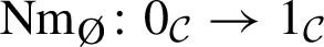
from the initial object to the terminal object of \({\mathcal {C}}\). Requiring this map to be an isomorphism is to require the existence of a zero object. Thus, \({\mathcal {C}}\) is \(\left( -1\right) \)-semiadditive if and only if it is pointed. This in turn allows us to integrate an empty family of morphisms. Namely, given \(X,Y\in {\mathcal {C}}\), we get a canonical zero map given by the composition

- (0):
-
A 0-finite space is one that is equivalent to a finite set A. Given a collection of objects \(\left\{ X_{a}\right\} _{a\in A}\) in a pointed \(\infty \)-category \({\mathcal {C}}\), we get a canonical map
$$\begin{aligned} {\text {Nm}}_{A}:\coprod _{a\in A}X_{a}\rightarrow \prod _{a\in A}X_{a}. \end{aligned}$$This map is given by the “identity matrix” (this uses the zero maps, which in turn use the inverse of
 ). Requiring these maps to be isomorphisms is precisely the usual property of being semiadditive, which allows one to sum a finite family of morphisms.
 - (1):
-
A connected 1-finite space is of the form \(A=BG\) for a finite group G. A diagram \(F:BG\rightarrow {\mathcal {C}}\) is equivalent to an object \(X\in {\mathcal {C}}\) equipped with an action of G. When \({\mathcal {C}}\) is semiadditive, one can construct the canonical norm map
$$\begin{aligned} {\text {Nm}}_{BG}:X_{hG}\rightarrow X^{hG} \end{aligned}$$and it can be identified with the classical norm of G. If \({\mathcal {C}}\) is stable, then \({\text {Nm}}_{BG}\) is an isomorphism if and only if its cofiber, the Tate construction \(X^{tG}\), vanishes. It is in this form that Theorems 1.1.1 and 1.1.4 were originally stated and proved.
 . The associated norm map is the unique map

 ). Requiring these maps to be isomorphisms is precisely the usual property of being semiadditive, which allows one to sum a finite family of morphisms.
1.2.4 Relative and axiomatic integration
Just like with ordinary semiadditivity, integration of m-finite families of maps satisfies various compatibilities. These generalize associativity, changing summation order, distributivity with respect to composition, etc. To conveniently manage those compatibility relations it is useful to extend the integral operation to the relative case. Given a map of m-finite spaces \(q:A\rightarrow B\), the pullback along q functor
admits a left and right adjoint, which we denote by \(q_{!}\) and \(q_{*}\) respectively. If \({\mathcal {C}}\) is \(\left( m-1\right) \)-semiadditive, one can construct a canonical norm map \({\text {Nm}}_{q}:q_{!}\rightarrow q_{*}\) and it is an isomorphism when \({\mathcal {C}}\) is m-semiadditive. Similarly to the absolute case, given objects \(X,Y\in {\text {Fun}}\left( B,{\mathcal {C}}\right) \), one can use the inverse of \({\text {Nm}}_{q}\) to define “integration along the fibers of q”,
The approach we take in this paper is to further generalize the situation and to put it in an axiomatic framework. We define a normed functor
to be a functor \( q^{*}:{\mathcal {C}}\rightarrow {\mathcal {D}}, \) that admits a left adjoint \(q_{!}\), a right adjoint \(q_{*}\), and is equipped with a natural transformation \({\text {Nm}}_{q}:q_{!}\rightarrow q_{*}\). If this natural transformation is an isomorphism, we can use the same formulas as above to define an abstract integration operation
for all \(X,Y\in {\mathcal {C}}\). We proceed to develop a general calculus of normed functors and integration, which can then be applied to the context of higher semiadditivity. One advantage of this axiomatic approach, is that it separates the formal aspects of this “calculus” from the rather involved inductive construction of the canonical norm maps. Another advantage is that it unifies many seemingly different phenomena as special cases of several general formal statements. This renders the development of the theory more economic and streamlined. Finally, we believe that this axiomatic framework might be of use elsewhere.
1.3 Outline of the proof
The core result of this paper is the \(\infty \)-semiadditivity of \({\text {Sp}}_{T\!\left( n\right) }\). For the convenience of the reader, we shall now sketch the proof. The argument is inductive on the level of semiadditivity m. The basis of the induction is \(m=1\), which is given by Theorem 1.1.4. Assume that \({\text {Sp}}_{T\left( n\right) }\) is m-semiadditive. In order to show that \({\text {Sp}}_{T\left( n\right) }\) is \(\left( m+1\right) \)-semiadditive, we need to prove that for every \(\left( m+1\right) \)-finite space B, the natural transformation  is an isomorphism. We proceed by a sequence of reductions. First, since \({\text {Sp}}_{T\left( n\right) }\) is stable and p-local, by [20, Proposition 4.4.16], it suffices to show that
(1) The norm map \({\text {Nm}}_{B}\) is an isomorphism for the single space \(B=B^{m+1}C_{p}\).
Now, consider a fiber sequence of spaces
where A and E are m-finite, and B is connected and \(\left( m+1\right) \)-finite. We prove that if the natural transformation |A| is invertible (we call such A amenable), then \({\text {Nm}}_{B}\) is an isomorphism (Proposition 3.1.18). In fact, it suffices to show that the component of |A| at the monoidal unit \(\mathbb {S}_{T\left( n\right) }\) is invertible (Lemma 3.3.5). By abuse of notation, we denote this component also by |A|.
In order to apply the above to \(B=B^{m+1}C_{p}\), we introduce the following class of “candidates” for A. We call a space A, m-good if it is connected, m-finite with \(\pi _{m}A\ne 0\), and all homotopy groups of A are p-groups. Since such A is in particular nilpotent, one can always fit it in a fiber sequence \(\left( *\right) \) with \(B=B^{m+1}C_{p}\). Thus, we are reduced to showing that
(2) There exists an m-good space A, such that \(|A|\in \pi _{0}\mathbb {S}_{T\left( n\right) }\) is invertible.
To detect invertibility in the ring \(\pi _{0}\mathbb {S}_{T\left( n\right) }\), we transport the problem into a better understood setting. Let \(E_{n}\) be the Morava E-theory \(\mathbb {E}_{\infty }\)-ring spectrum of height n, and let \({\widehat{{\text {Mod}}}}_{E_n}\) be the \(\infty \)-category of \(K\!\left( n\right) \)-local \(E_{n}\)-modules. The functor
is symmetric monoidal, and hence induces a map of commutative rings
Using the Nilpotence Theorem and standard techniques of chromatic homotopy theory, we show that an element of \(\pi _{0}\mathbb {S}_{T\left( n\right) }\) is invertible, if and only if its image under f is invertible (Corollary 5.1.17). Moreover, the functor \(E_{n}{\widehat{\otimes }}\left( -\right) \) is colimit preserving. Thus, by general arguments of higher semiadditivity we can deduce that \({\widehat{{\text {Mod}}}}_{E_n}\) is also m-semiadditive (Corollary 3.3.2(2)), and moreover, \(f\left( |A|\right) \) coincides with the element |A| of \(\pi _{0}E_{n}\) (Corollary 3.2.7). Thus, we can replace \({\text {Sp}}_{T\left( n\right) }\) with the more approachable \(\infty \)-category \({\widehat{{\text {Mod}}}}_{E_n}.\) Namely, it suffices to show
(3) There exists an m-good space A, such that \(|A|\in \pi _{0}E_{n}\) is invertible.
By [5, Lemma 1.33], the image of f is contained in the constants \(\mathbb {Z}_{p}\). Hence, |A| is invertible, if and only if its p-adic valuation is zero. On \(\mathbb {Z}_{p},\) we have the Fermat quotient operation
with the salient property of reducing the p-adic valuation of non-invertible non-zero elements. The heart of the proof comprises of realizing the algebraic operation \({\tilde{\delta }}\) in a way that acts on the elements |A| in an understood way. It is for this step that it is crucial that our induction base is \(m=1\). Namely, for a presentable, 1-semiadditive, stable, p-local, symmetric monoidal \(\infty \)-category \(({\mathcal {C}},\otimes , \mathbbm {1}_{{\mathcal {C}}})\), we construct a “power operation” (Definition 4.1.1 and Theorem 4.3.2)
that shares many of the formal properties of \({\tilde{\delta }}\). In particular, specializing to the case \({\mathcal {C}}={\widehat{{\text {Mod}}}}_{E_n}\), the operation \(\delta \) coincides with \({\tilde{\delta }}\) on \(\mathbb {Z}_{p}\subseteq \pi _{0}E_{n}\). Moreover, for an m-good A, we have
where \(A'\) and \(A''\) are also m-good (combine Definition 4.3.1 and Theorem 4.2.13). It follows that if |A| is non-zero (and not already invertible), then at least one of \(|A'|\) and \(|A''|\) has lower p-adic valuation than |A|. The prototypical m-good space is the Eilenberg–MacLane space \(B^{m}C_{p}\). Hence, it suffices to show that
(4) The element \(|B^{m}C_{p}|\in \pi _{0}E_{n}\) is non-zero.
To get a grip on the elements |A|, we reformulate them in terms of the symmetric monoidal dimension, which does not refer at all to higher semiadditivity.Footnote 6 Let us denote by \(A\otimes E_{n}\), the colimit of the constant A-shaped diagram on \(E_{n}\) in \({\widehat{{\text {Mod}}}}_{E_n}\). We show that \(A\otimes E_{n}\) is a dualizable object,Footnote 7 and that (Corollary 3.3.12)
Since
it suffices to show that
(5) The element \(\dim \left( B^{m}C_{p}\otimes E_{n}\right) \in \pi _{0}E_{n}\) is non-zero.
Finally, it can be shown that \(\dim \left( A\otimes E_{n}\right) \) equals the Euler characteristic of the 2-periodic Morava K-theory (Lemma 5.1.7)Footnote 8
Hence, it suffices to prove that
(6) The integer \(\chi _{n}\left( B^{m}C_{p}\right) \) is non-zero.
This is an immediate consequence of the explicit computation of \(K\!\left( n\right) _{*}(B^{m}C_{p})\), carried out in [45].
We alert the reader that at several points, this outline diverges from the actual proof we give. Most significantly, we make use of the fact that the steps (1)–(5) are completely formal and the ideas involved can be formalized in a much greater generality. Instead of the functor \(E_{n}{\widehat{\otimes }}\left( -\right) \), we can consider any colimit preserving symmetric monoidal functor \(F:{\mathcal {C}}\rightarrow {\mathcal {D}}\) between stable, p-local, symmetric monoidal \(\infty \)-categories. Given such a functor F, we show how to bootstrap 1-semiadditivity to higher semiadditivity under appropriate conditions (Theorem 4.3.10). This necessitates some technical changes in the argument outlined above.Footnote 9 It is only in the final section that we specialize to \({\mathcal {C}}={\text {Sp}}_{T\left( n\right) }\), and verify the assumptions of this general criterion.
1.4 Organization
We now describe the content of each section of the paper.
In Sect. 2, we develop the axiomatic framework of normed functors and integration. We begin by developing some general calculus for this notion and study its functoriality properties. We then study the interaction of integration with symmetric monoidal structures and the notion of duality. We conclude with a discussion of the property of amenability.
In Sect. 3, we apply the axiomatic theory of Sect. 2 to the setting of local systems valued in an m-semiadditive \(\infty \)-category. We begin by recalling the canonical norm on the pullback functor along an m-finite map (introduced in [20, §4.1]), and its interaction with various operations. We then consider m-finite colimit preserving functors between m-semiadditive \(\infty \)-categories (a.k.a m-semiadditive functors), and their behavior with respect to integration. We continue with studying the interaction of m-semiadditivity with symmetric monoidal structures, duality, and dimension. Finally, we study the behavior of equivariant powers in 1-semiadditive \(\infty \)-categories, which is used in the sequel in the construction of power operations.
In Sect. 4, we construct the above-mentioned power operations for 1-semiadditive stable \(\infty \)-categories. First, we introduce the algebraic notion of an additive p-derivation and study some of its properties. We then construct an auxiliary operation \(\alpha \) in the presence of 1-semiadditivity. Specializing to the stable (p-local) case, we construct from \(\alpha \) the additive p-derivation \(\delta \) and establish its naturality properties. Finally, we formulate and prove the “bootstrap machine”, that gives general conditions for a 1-semiadditive \(\infty \)-category to be \(\infty \)-semiadditive. We conclude the section with a discussion of “nil-conservativity” which is a natural setup to which one can apply the bootstrap machine. In Sect. 5, we apply the abstract theory of Sects. 2–4 to chromatic homotopy theory. After some generalities, we use the additive p-derivation of Sect. 4 to derive a generalization of a conjecture of May about nilpotence in \(H_{\infty }\)-rings. We then apply the “bootstrap machine” to the 1-semiadditive \(\infty \)-category \({\text {Sp}}_{T\!\left( n\right) }\), to show that it is \(\infty \)-semiadditive, and deduce that \(T\!\left( n\right) \)-homology of \(\pi \)-finite spaces depends only on the nth Postnikov truncation. Finally, we consider localizations with respect to general weak rings. We show, among other things, that in this setting 1-semiadditivity implies \(\infty \)-semiadditivity, and that various notions of “bounded height” coincide.
1.5 Terminology and notation
Throughout the paper we work in the framework of \(\infty \)-categories (a.k.a. quasicategories), introduced by A. Joyal [27], and extensively developed by Lurie in [31, 32]. We shall also use the following terminology and notation:
-
(1)
We use the term isomorphism for an invertible morphism of an \(\infty \)-category (i.e. an equivalence).
-
(2)
We say that a space A is
-
(a)
\(\left( -2\right) \)-finite, if it is contractible.
-
(b)
m-finite for \(m\ge -1\), if \(\pi _{0}A\) is finite and all the fibers of the diagonal map \(\Delta _{A}:A\rightarrow A\times A\) are \(\left( m-1\right) \)-finite (for \(m\ge 0\), this is equivalent to A having finitely many components, each of them m-truncated with finite homotopy groups).
-
(c)
\(\pi \)-finite, if it is m-finite for some integer \(m\ge -2\).
-
(a)
-
(3)
We say that a \(\pi \)-finite space A is a p-space, if all the homotopy groups of A are p-groups.
-
(4)
Given a map of spaces \(q:A\rightarrow B\), for every \(b\in B\) we denote by \(q^{-1}\left( b\right) \) the homotopy fiber of q over b.
-
(5)
For \(m\ge -2\), we say that a map of spaces \(q:A\rightarrow B\) is m-finite (resp. \(\pi \)-finite) if \(q^{-1}(b)\) is m-finite (resp. \(\pi \)-finite) for all \(b\in B\).
-
(6)
Given an \(\infty \)-category \({\mathcal {C}}\), we say that \({\mathcal {C}}\) admits all q-limits (resp. q-colimits) if it admits all limits (resp. colimits) of shape \(q^{-1}\left( b\right) \) for all \(b\in B\).
-
(7)
Given a functor \(F:{\mathcal {C}}\rightarrow {\mathcal {D}}\) of \(\infty \)-categories, we say that F preserves q-colimits (resp. q-limits) if it preserves all colimits (resp. limits) of shape \(q^{-1}\left( b\right) \) for all \(b\in B\).
-
(8)
We use the notation

to denote that \(f:X\rightarrow Z\) is the composition \(h\circ g\) (which is well defined up to a contractible space of choices). We use similar notation for composition of more than two morphisms.
-
(9)
Given functors \(F,G:{\mathcal {C}}\rightarrow {\mathcal {D}}\) and \(H,K:{\mathcal {D}}\rightarrow {\mathcal {E}}\), and natural transformations \(\alpha :F\rightarrow G\) and \(\beta :H\rightarrow K\), we denote their horizontal composition by \(\beta \star \alpha :HF\rightarrow KG\). The vertical composition of natural transformations is denoted simply by juxtaposition.
-
(10)
For a symmetric monoidal \(\infty \)-category \({\mathcal {C}}\), we denote by \({\text {CAlg}}({\mathcal {C}})\) the \(\infty \)-category of \({\mathbb {E}}_{\infty }\)-algebras in \({\mathcal {C}}\). We denote \({\text {coCAlg}}({\mathcal {C}})={\text {CAlg}}({\mathcal {C}}^{op})^{op}\) the \(\infty \)-category of \(\mathbb {E}_{\infty }\)-coalgebras in \({\mathcal {C}}\), where \({\mathcal {C}}^{op}\) is endowed with the canonical symmetric monoidal structure induced from \({\mathcal {C}}\).
-
(11)
For an abelian group A and \(k\ge 0\), we denote by \(B^{k}A\) the Eilenberg MacLane space with kth homotopy group equal to A.

2 Norms and integration
In this section, we develop an abstract formal framework of norms on functors between \(\infty \)-categories and the operation of integration on maps, that such norms induce. This framework abstracts, axiomatizes, and generalizes the theory of norms and integrals arising from ambidexterity developed in [20, §4]. We develop a “calculus” for such integrals and study their functoriality properties and interaction with monoidal structures.
2.1 Normed functors and integration
2.1.1 Norms and iso-norms
We begin by fixing some terminology regarding adjunctions of \(\infty \)-categories.
Definition 2.1.1
Let \(F:{\mathcal {C}}\rightarrow {\mathcal {D}}\) be a functor of \(\infty \)-categories.
-
(1)
By a left adjoint to F, we mean a pair \(\left( L,u\right) \), where \(L:{\mathcal {D}}\rightarrow {\mathcal {C}}\) is a functor and
$$\begin{aligned} u:{\text {Id}}_{{\mathcal {D}}}\rightarrow F\circ L \end{aligned}$$is a unit natural transformation in the sense of [32, Definition 5.2.2.7].
-
(2)
By a right adjoint to F, we mean a pair \(\left( R,c\right) \), where \(R:{\mathcal {D}}\rightarrow {\mathcal {C}}\) is a functor and
$$\begin{aligned} c:F\circ R\rightarrow {\text {Id}}_{{\mathcal {D}}} \end{aligned}$$a counit natural transformation (i.e. satisfying the dual of [32, Definition 5.2.2.7]).
Remark 2.1.2
Given a datum of a left adjoint \(\left( L,u\right) \), there exists a map \(c:L\circ F\rightarrow {\text {Id}}_{{\mathcal {C}}}\), such that u and c satisfy the zig-zag identities up to homotopy. From this also follows that c is a counit map exhibiting \(\left( F,c\right) \) as a right adjoint to L. This counit map c is unique up to homotopy, and we shall therefore sometimes speak of “the” associated counit map. In fact, the space of such maps together with a homotopy witnessing one of the zig-zag identities is contractible [44, Proposition 4.4.7]. We shall similarly speak of the unit map \(u:{\text {Id}}_{{\mathcal {C}}}\rightarrow R\circ F\) associated with a right adjoint \(\left( R,c\right) \).
Adjoint functors can be composed in the following (usual) sense:
Definition 2.1.3
As in [33, Tag 02ES], given a pair of composable functors

with left adjoints \(\left( L,u\right) \) and \(\left( L',u'\right) \) respectively, the composite map

which is well defined up to homotopy, is a unit map exhibiting \(LL'\) as left adjoint to \(F'F\). We define the counit map of the composition of right adjoints in a similar way.
The central notion we are about to study in this section is the following:
Definition 2.1.4
Given \(\infty \)-categories \({\mathcal {C}}\) and \({\mathcal {D}}\), a normed functor
is a functor \(q^{*}:{\mathcal {C}}\rightarrow {\mathcal {D}}\) together with a left adjoint \(\left( q_{!},u_{!}^{q}\right) \), a right adjoint \(\left( q_{*},c_{*}^{q}\right) \), and a natural transformation
which we call a norm. We say that q is iso-normed, if \({\text {Nm}}_{q}\) is a natural isomorphism. For \(X\in {\mathcal {C}}\), we also write \(X_{q}=q_{!}q^{*}X\), and denote by \(c_{!}^{q}:q_{!}q^{*}\rightarrow {\text {Id}}\) and \(u_{*}^{q}:{\text {Id}}\rightarrow q_{*}q^{*}\), the associated counit and unit of the respective adjunctions. We drop the superscript q whenever it is clear from the context.
Iso-normed functors have also been called ambidextrous adjunctions in the literature, see e.g. [30], and appear in classical mathematical contexts, such as algebraic geometry and representation theory.
Example 2.1.5
For an inclusion of finite groups \(H\subseteq G\), the restriction functor from complex G-representations to H-representations extends naturally to an iso-normed functor. Namely, there is a natural isomorphism between induction and co-induction from H to G.
Remark 2.1.6
In subsequent sections, we shall sometimes abuse language and refer to \({\text {Nm}}_{q}\) as a norm on \(q^{*}\) and to \(q^{*}\) itself (with the data of \({\text {Nm}}_{q}\)) as a normed functor. Since the left and right adjoints of \(q^{*}\) are essentially unique (when they exist), this seems to be a rather harmless convention.
There is a useful criterion for detecting when a normed functor is iso-normed.
Lemma 2.1.7
A normed functor \(q:{\mathcal {D}}\rightarrowtail {\mathcal {C}}\) is iso-normed if and only if the norm \({\text {Nm}}_{q}:q_{!}\rightarrow q_{*}\) is an isomorphism at \(q^{*}X\) for all \(X\in {\mathcal {C}}\).
Proof
The “only if” part is clear. For the “if” part, consider the two diagrams

which commute by naturality of the (co)unit maps. By the zig-zag identities, the composition along the bottom row in the left diagram is the identity. Thus, the left diagram shows that \({\text {Nm}}_{q}\) has a right inverse. Similarly, the right diagram shows that \({\text {Nm}}_{q}\) has a left inverse and therefore \({\text {Nm}}_{q}\) is an isomorphism. \(\square \)
Given a functor \(q^{*}:{\mathcal {C}}\rightarrow {\mathcal {D}}\) with a left adjoint \(\left( q_{!},u_{!}^{q}\right) \) and a right adjoint \(\left( q_{*},c_{*}^{q}\right) \), the data of a natural transformation \({\text {Nm}}_{q}:q_{!}\rightarrow q_{*}\) is equivalent to the data of its mate \(\nu _{q}:q^{*}q_{!}\rightarrow {\text {Id}}\), which is a candidate for a counit of a “wrong way” adjunction \(q^* \dashv q_!\).
Lemma 2.1.8
Let \(q:{\mathcal {D}}\rightarrowtail {\mathcal {C}}\) be a normed functor. For every \(Y\in {\mathcal {D}}\), the map \({\text {Nm}}_{q}:q_{!}\rightarrow q_{*}\) is an isomorphism at \(Y\in {\mathcal {D}}\) if and only if the mate \(\nu _{q}:q^{*}q_{!}\rightarrow {\text {Id}}\) is a counit map at Y; That is, for all \(X\in {\mathcal {C}}\), the composition

is a homotopy equivalence.
Proof
For every \(X\in {\mathcal {C}}\), consider the commutative diagram in the homotopy category of spaces:

By the Yoneda lemma, \({\text {Nm}}_{q}\) is an isomorphism at Y if and only if the top map in the diagram is an isomorphism for all \(X\in {\mathcal {C}}\). By 2-out-of-3, this is the case if and only if the composition of the top map and the diagonal map is an isomorphism for all X. Since the diagram commutes, this is if and only if the composition of the left vertical map with the long bottom map is an isomorphism for all X, which is by definition if and only if \(\nu _{q}\) is a counit at Y.
\(\square \)
Notation 2.1.9
When \({\text {Nm}}_{q}\) is an isomorphism at \(q^*X\), and hence \(\nu _{q}\) is a counit at X, we denote the associated unit by \(\mu _{q,X}:X\rightarrow q_{!}q^{*}X=X_{q}\). If q is iso-normed, we let \(\mu _{q}:{\text {Id}}\rightarrow q_{!}q^{*}\) be the unit natural transformation associated with \(\nu _{q}\). As usual, we drop the subscript q, whenever the map is understood from the context.
Remark 2.1.10
We will use the two points of view, that of a norm \({\text {Nm}}_{q}:q_{!}\rightarrow q_{*}\) and that of a “wrong way counit” \(\nu _{q}:q^{*}q_{!}\rightarrow {\text {Id}}\) interchangeably. Each point of view has its own advantages. We note that the definition using \(\nu _{q}\) seems to be slightly more general as it is available even if \(q^{*}\) does not (a priori) admit a right adjoint. In practice, we are mainly interested in situations where \(\nu _{q}\) is indeed a counit map for an adjunction, exhibiting \(q_{!}\) as a right adjoint of \(q^{*}\). Thus, the gain in generality is rather negligible.
Definition 2.1.11
We define the identity normed functor and composition of normed functors (up to homotopy) as follows.
-
(1)
(Identity) For every \(\infty \)-category \({\mathcal {C}}\), the identity normed functor \({\text {Id}}:{\mathcal {C}}\rightarrowtail {\mathcal {C}}\) consists of the identity functor \({\text {Id}}:{\mathcal {C}}\rightarrow {\mathcal {C}}\) viewed as a left and right adjoint to itself using the identity natural transformation \({\text {Id}}\rightarrow {\text {Id}}\) as the (co)unit map and with the identity natural transformation \({\text {Id}}\rightarrow {\text {Id}}\) as the norm.
-
(2)
(Composition) Given a pair of composable normed functors

we define their composition \(qp:{\mathcal {E}}\rightarrowtail {\mathcal {C}}\) by composing the adjunctions (Definition 2.1.3)
$$\begin{aligned} \left( qp\right) ^{*}=p^{*}q^{*},\quad \left( qp\right) _{!}=q_{!}p_{!}, \quad \left( qp\right) _{*}=q_{*}p_{*} \end{aligned}$$and take the norm map to be the horizontal composition of the norms (the order does not matter)

We denote the norm of the composite by \({\text {Nm}}_{qp}\). If p and q are iso-normed, then so is qp.


Remark 2.1.12
It is possible to define an \(\infty \)-category \({\widehat{\mathbf {Cat}}}_{\infty }^{{\text {Nm}}}\), whose objects are \(\infty \)-categories and morphisms are normed functors, such that the above constructions give the identity morphisms and composition in the homotopy category. This \(\infty \)-category captures the higher coherences manifest in the above definitions. We intend to elaborate on this point in a future work, but for the purposes of this one, which will not use the higher coherences in any way, we shall be content with the above explicit definitions up to homotopy.
2.1.2 Integration
The main feature of iso-normed functors is that they allow us to define a formal notion of “integration” of maps.
Definition 2.1.13
Let \(q:{\mathcal {D}}\rightarrowtail {\mathcal {C}}\) be an iso-normed functor. For every \(X,Y\in {\mathcal {C}}\), we define an integral map
which is natural in X and Y, as the composition

Remark 2.1.14
Alternatively, using the wrong way unit \(\mu _{q}:{\text {Id}}\rightarrow q_{!}q^{*}\), one can define the integral as the composition

As a special case we have
Definition 2.1.15
Let \(q:{\mathcal {D}}\rightarrowtail {\mathcal {C}}\) be an iso-normed functor. For every \(X\in {\mathcal {C}}\), we define a map
by
Remark 2.1.16
By unwinding the definition of the integral, the maps \(|q|_{X}:X\rightarrow X\) are the components of the natural endomorphism \(|q|=c_{!}^{q}\circ \mu _{q}\) of \({\text {Id}}_{{\mathcal {C}}}\).
Integration satisfies a form of “homogeneity”.
Proposition 2.1.17
(Homogeneity) Let \(q:{\mathcal {D}}\rightarrowtail {\mathcal {C}}\) be an iso-normed functor and let \(X,Y,Z\in {\mathcal {C}}\).
-
(1)
For all maps \(f:q^{*}X\rightarrow q^{*}Y\) and \(g:Y\rightarrow Z\) we have
$$\begin{aligned} g\circ \left( \int \limits _{q}f\right) =\int \limits _{q}\left( q^{*}g\circ f\right) \quad \in {\text {Hom}}_{h{\mathcal {C}}}\left( X,Z\right) . \end{aligned}$$ -
(2)
For all maps \(f:X\rightarrow Y\) and \(g:q^{*}Y\rightarrow q^{*}Z\) we have
$$\begin{aligned} \left( \int \limits _{q}g\right) \circ f=\int \limits _{q}\left( g\circ q^{*}f\right) \quad \in {\text {Hom}}_{h{\mathcal {C}}}\left( X,Z\right) . \end{aligned}$$
Proof
For (1), consider the commutative diagram

The composition along the top and then right path is \(g\circ \int \limits _{q}f\), while the composition along the left and then bottom path is \(\int \limits _{q}\left( q^{*}g\circ f\right) \), see Remark 2.1.14.
For (2), consider the diagram

and apply an analogous argument. \(\square \)
Integration also satisfies a form of “Fubini’s Theorem”.
Proposition 2.1.18
(Higher Fubini’s Theorem) Given a pair of composable iso-normed functors

for all \(X,Y\in {\mathcal {C}}\), and \(f:p^{*}q^{*}X\rightarrow p^{*}q^{*}Y\), we have
Proof
Since q and p are iso-normed, we can construct the following diagram

The triangles and the bottom right square commute for formal reasons. The top right square commutes by the way norms are composed (Definition 2.1.11(2)) and the left rectangle commutes by definition of \(\int \limits _{p}f\). Thus, the composition along the top path, which is \(\int \limits _{qp}f\), is homotopic to the composition along the bottom path, which is \(\int \limits _{q}\left( \int \limits _{p}f\right) \). \(\square \)
Remark 2.1.19
Fubini’s theorem for Kan extensions is a special case when \({\mathcal {C}}\) is the \(\infty \)-semiadditive \(\infty \)-category of co-complete \(\infty \)-categories and colimit preserving functors. This example is worked out in [13, §2.2].
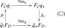
2.2 Ambidextrous squares and Beck–Chevalley conditions
In this section we study functoriality properties of norms and integrals and develop further the “calculus of integration”.
2.2.1 Beck–Chevalley conditions
We begin by recalling some standard material regarding commuting squares involving adjoint functors (e.g. see beginning of [32, §7.3.1]). A commutative square of functors

is a natural isomorphism

If the vertical functors admit left adjoints \(q_{!}\dashv q^{*}\) and \({\tilde{q}}_{!}\dashv {\tilde{q}}^{*}\) (suppressing the units), we get a \({\text {BC}}_{!}\) (Beck–Chevalley) natural transformation

Similarly, if the vertical functors admit right adjoints \(q^{*}\dashv q_{*}\) and \({\tilde{q}}^{*}\dashv {\tilde{q}}_{*}\), we get a \({\text {BC}}_{*}\) (Beck–Chevalley) natural transformation

Definition 2.2.1
We say that the square \(\square \) satisfies the \(\text {BC}_{!}\) (resp. \(\text {BC}_{*}\)) condition, if \(q^{*}\) and \({\tilde{q}}^{*}\) admit left (resp. right) adjoints and the map \(\beta _{!}\) (resp. \(\beta _{*}\)) is an isomorphism.
Example 2.2.2
A classical example of a square satisfying the \(\text {BC}_*\) is given by the proper-base change theorem, see [48, 095S] in the context of étale cohomology, and [32, Introduction to §7] in the context of locally compact Hausdorff spaces.
Warning 2.2.3
It may happen that in \(\square \), the horizontal functors \(F_{{\mathcal {C}}}\) and \(F_{{\mathcal {D}}}\) also have left or right adjoints. In this case, there are other BC maps one can write. To avoid confusion, we will always speak about the BC maps with respect to the vertical functors.
Given a commutative square \(\square \) as above, such that \(q^*\) and \({\tilde{q}}^*\) admit right adjoints, we denote \(u_{*}=u_{*}^{q}\) and \({\tilde{u}}_{*}=u_{*}^{{\tilde{q}}}\) (and similarly for other (co)unit maps). It is an easy verification using the zig-zag identities, that the BC-maps are compatible with these units and counits in the following sense:
Lemma 2.2.4
Given a commutative square of functors \(\square \), such that \(q^{*}\) and \({\tilde{q}}^{*}\) admit left (resp. right) adjoints, the following four diagrams commute up to homotopy:

The \({\text {BC}}\) maps also satisfy some naturality properties with respect to horizontal and vertical pasting, as well as multiplication and exponentiation of squares. We begin with horizontal pasting. Given a commutative diagram of \(\infty \)-categories and functors

we call the outer square the horizontal pasting of the left and right small squares. The following is easy to verify.
Lemma 2.2.5
Given a horizontal pasting diagram \(\left( *\right) \) as above,
-
(1)
The \({\text {BC}}_{!}\)-map for the outer square is homotopic to the composition

of the \({\text {BC}}_{!}\) maps for the left and right squares.
-
(2)
The \({\text {BC}}_{*}\)-map for the outer square is homotopic to the composition

of the \({\text {BC}}_{*}\) maps for the left and right squares.


This immediately implies the following horizontal pasting lemma for \({\text {BC}}\) conditions.
Corollary 2.2.6
Given a horizontal pasting diagram \(\left( *\right) \) as above, denote by \(\square _{L}\), \(\square _{R}\) and \(\square \), the left, right and outer squares respectively.
-
(1)
If \(\square _{L}\) and \(\square _{R}\) satisfy the \({\text {BC}}_{!}\) (resp. \({\text {BC}}_{*}\)) condition, then so does \(\square \).
-
(2)
If \(\square _{R}\) and \(\square \) satisfy the \({\text {BC}}_{!}\) (resp. \({\text {BC}}_{*}\)) condition and \(G_{{\mathcal {C}}}\) is conservative, the so does \(\square _{L}\).
We now turn to vertical pasting. Given a commutative diagram of \(\infty \)-categories and functors

we call the big outer square (i.e. rectangle) the vertical pasting of the top and bottom small squares. The following is easy to verify.
Lemma 2.2.7
Given a vertical pasting diagram \(\left( **\right) \) as above,
-
(1)
The \({\text {BC}}_{!}\)-map for the outer square is homotopic to the composition of the \({\text {BC}}_{!}\) maps for the top and bottom squares

-
(2)
The \({\text {BC}}_{*}\)-map for the outer square is homotopic to the composition of the \({\text {BC}}_{*}\) maps for the top and bottom squares


Again, this immediately implies the following vertical pasting lemma for \({\text {BC}}\) conditions.
Corollary 2.2.8
Given a vertical pasting diagram \(\left( **\right) \) as above, denote by \(\square _{T}\), \(\square _{B}\) and \(\square \), the top, bottom, and outer squares respectively. If \(\square _{T}\) and \(\square _{B}\) satisfy the \({\text {BC}}_{!}\) (resp. \({\text {BC}}_{*}\)) condition, then so does \(\square \).
Finally, the \({\text {BC}}\) conditions are also natural with respect to multiplication and exponentiation.
Lemma 2.2.9
Given a pair of squares corresponding under the adjunction \( (-)\times {\mathcal {E}} \dashv {\text {Fun}}({\mathcal {E}},-), \)

the square \(\square _{1}\) satisfies the \({\text {BC}}_{!}\) (resp. \({\text {BC}}_{*}\)) if and only if \(\square _{2}\) satisfies the \({\text {BC}}_{!}\) (resp. \({\text {BC}}_{*}\)) condition.
Proof
Under the canonical equivalence of \(\infty \)-categories
the \(\text {BC}_{!}\) (resp. \(\text {BC}_{*}\)) map for \(\square _{1}\) corresponds to the \(\text {BC}_{!}\) (resp. \(\text {BC}_{*}\)) map of \(\square _{2}\) and isomorphisms correspond to isomorphisms. \(\square \)
2.2.2 Normed and ambidextrous squares
We now consider commuting squares of \(\infty \)-categories, where the vertical functors are normed.
Definition 2.2.10
We define:
-
(1)
A normed square is a pair of normed functors \(q:{\mathcal {D}}\rightarrowtail {\mathcal {C}}\) and \({\tilde{q}}:\tilde{{\mathcal {D}}}\rightarrowtail \tilde{{\mathcal {C}}}\), together with a commutative diagram

It is iso-normed if q and \({\tilde{q}}\) are iso-normed.
-
(2)
A weakly ambidextrous square is a normed square, such that the associated norm diagram:
commutes up to homotopy. An ambidextrous square is a weakly ambidextrous square that is iso-normed (note that an ambidextrous square satisfies the \({\text {BC}}_{!}\) condition if and only if it satisfies the \({\text {BC}}_{*}\) condition).


Remark 2.2.11
We shall often abuse language and say that \(\left( *\right) \) is a normed (or ambidextrous) square implying by this that we also have normed functors q and \({\tilde{q}}\) as in the definition.
As with any definition regarding norms, we can recast the definition of an ambidextrous square in terms of wrong way counits. As this will be used in the sequel, we shall spell this out.
Lemma 2.2.12
Let \(\left( *\right) \) be a normed square as in Definition 2.2.10(1). Consider the diagrams (where
 is defined only when
\(\left( *\right) \) is iso-normed).
is defined only when
\(\left( *\right) \) is iso-normed).

-
(1)
The norm-diagram \(\square \) commutes if and only if the diagram
 commutes.
 -
(2)
If \(\left( *\right) \) is iso-normed, satisfies the \({\text {BC}}_{!}\) condition and the norm-diagram \(\square \) commutes, then the diagram
 commutes.
 commutes.
 commutes.
Proof
We begin with (1). The norm-diagram \(\square \) commutes if and only if the two maps \({\tilde{q}}_{!}F_{{\mathcal {D}}}\rightarrow {\tilde{q}}_{*}F_{{\mathcal {D}}}\) are homotopic. This holds if and only if their mates \({\tilde{q}}^{*}{\tilde{q}}_{!}F_{{\mathcal {D}}}\rightarrow F_{{\mathcal {D}}}\) are homotopic. To compute the mate, one applies \({\tilde{q}}^{*}\) and post-composes with the counit \({\tilde{c}}_{*}:{\tilde{q}}^{*}{\tilde{q}}_{*}\rightarrow {\text {Id}}\) (of the right way adjunction). Now, consider the diagram

The triangle on the right commutes by Lemma 2.2.4(2). The composition of the top maps is \(F_{{\mathcal {D}}}\nu _{q}\) and of the bottom maps is \(\nu _{{\tilde{q}}}F_{{\mathcal {D}}}\). Hence, \(\square \) commutes, if and only if  commutes.
We now turn to (2). To check the commutativity of  , we may replace \(\beta _{!}\) with its inverse. By assumption, all maps in \(\square \) are isomorphisms. Thus, the map \(\beta _{!}^{-1}\) in
  is homotopic to the composition

Unwinding the definitions, this exhibits \(\beta _{!}^{-1}\) as the \({\text {BC}}_{*}\)-map of the wrong way adjunctions \(q^{*}\dashv q_{!}\) and \({\tilde{q}}^{*}\dashv {\tilde{q}}_{!}\). The commutativity of  now follows from the compatibility of \({\text {BC}}\)-maps with units (Lemma 2.2.4(1)). \(\square \)
The main feature of ambidextrous squares is that they behave well with respect to the integral operation.
Proposition 2.2.13
Let

be an ambidextrous square that satisfies the \({\text {BC}}_{!}\) condition (and hence the \({\text {BC}}_{*}\) condition). For all \(X,Y\in {\mathcal {C}}\) and \(f:q^{*}X\rightarrow q^{*}Y,\) we have
In particular, for all \(X\in {\mathcal {C}}\), we have
Proof
Since \(\square \) is iso-normed, we can construct the following diagram:

The left and right triangles commute by the compatibility of \({\text {BC}}\) maps with (co)units (Lemma 2.2.4, diagrams (1), and (4) respectively). The top right square commutes by the assumption that the square \(\square \) is ambidextrous and satisfies the \({\text {BC}}\) conditions and the rest of the squares commute for trivial reasons. Hence, the composition along the top path is homotopic to the composition along the bottom path, which proves the first claim. The second claim follows from the first applied to the map \(f=q^{*}{\text {Id}}_{X}\). \(\square \)
2.2.3 Calculus of normed squares
As discussed before, squares of functors can be pasted horizontally and vertically. We extend these operations to normed squares and consider their compatibility with the notion of ambidexterity. We begin with horizontal pasting. Given normed functors
and a commutative diagram

we call the big outer normed square the horizontal pasting of the left and right small normed squares. We have the following horizontal pasting lemma for ambidexterity.
Lemma 2.2.14
(Horizontal Pasting)Let \(\left( *\right) \) be a horizontal pasting diagram of normed squares as above. We denote by \(\square _{L}\), \(\square _{R}\) and \(\square \), the left, right, and outer normed squares respectively. If \(\square _{L}\) and \(\square _{R}\) are (weakly) ambidextrous, then so is \(\square \).
Proof
Consider the following diagram composed of whiskerings of the norm diagrams of \(\square _{L}\) and \(\square _{R}\) (with all horizontal maps the respective \({\text {BC}}\)-maps).

By Lemma 2.2.5, the outer square is the norm diagram for \(\square \), which implies the claim. \(\square \)
We now turn to vertical pasting. Given normed functors
and a commutative diagram

we call the big outer normed square, with respect to the compositions of normed functors qp and \({\tilde{q}}{\tilde{p}}\), the vertical pasting of the top and bottom small normed squares. We have the following vertical pasting lemma for ambidexterity:
Lemma 2.2.15
(Vertical Pasting) Let \(\left( **\right) \) be a vertical pasting diagram of normed squares as above. We denote by \(\square _{T}\), \(\square _{B}\) and \(\square \), the top, bottom, and outer normed squares respectively. If \(\square _{T}\) and \(\square _{B}\) are (weakly) ambidextrous, then so is \(\square \).
Proof
Consider the following diagram composed of whiskerings of the norm diagrams of \(\square _{T}\) and \(\square _{B}\) (with all horizontal maps the respective \({\text {BC}}\)-maps).

By Lemma 2.2.7, the outer diagram is the norm diagram for \(\square \). Thus, it is enough to check that all four small squares commute. The top right and bottom left squares commute for trivial reasons. The top left and bottom right squares are whiskerings of the norm diagrams of \(\square _{T}\) and \(\square _{B}\) respectively and hence commute by assumption. \(\square \)
2.3 Monoidal structure and duality
In this section, we study the interaction of norms and integration with (symmetric) monoidal structures on the source and target \(\infty \)-categories. Under suitable hypotheses, this interaction allows us to reduce questions about ambidexterity to questions about duality.
2.3.1 Tensor normed functors
Definition 2.3.1
Let \({\mathcal {C}}\) and \({\mathcal {D}}\) be monoidal \(\infty \)-categories. A \(\otimes \)-normed functor from \({\mathcal {D}}\) to \({\mathcal {C}}\), is a normed functor \(q:{\mathcal {D}}\rightarrowtail {\mathcal {C}}\), such that \(q^{*}\) is monoidal (and hence \(q_{!}\) is colax monoidal by the dual of [31, Corollary 7.3.2.7]) and for all \(Y\in {\mathcal {D}}\) and \(X\in {\mathcal {C}}\), the compositions of the canonical maps

and

are isomorphisms.
Remark 2.3.2
The above definition does not depend on the norm and is actually just a property of the functor \(q^{*}\). However, we shall only be interested in this property in the context of normed functors.
Remark 2.3.3
The analogous property with \(q_*\) instead of \(q_!\) is commonly referred to as the projection formula. A classical example is the projection formula for coherent sheaves on schemes, see [48, 01E6].
Notation 2.3.4
To make diagrams involving (co)units more readable, we shall employ the following graphical convention. When writing a unit map of an adjunction whiskered by some functors, we enclose in parenthesis the effected terms in the target. Similarly, when writing a counit map of an adjunction whiskered by some functors, we underline the effected terms in the source.
We adopt the definitions and terminology of [20] regarding duality in monoidal \(\infty \)-categories. In the situation of Definition 2.3.1, substituting \(q^*\mathbbm {1}_{{\mathcal {C}}}\) for Y, gives a natural isomorphism from the functor \(q_{!}q^{*}\) to the functor \(\mathbbm {1}_{q}\otimes -\), where \(\mathbbm {1}_{q}=q_{!}q^{*}\mathbbm {1}_{{\mathcal {C}}}\). We can therefore consider the map

Proposition 2.3.5
Let \(q:{\mathcal {D}}\rightarrowtail {\mathcal {C}}\) be a \(\otimes \)-normed functor of monoidal \(\infty \)-categories. The following are equivalent:
-
(1)
\({\text {Nm}}_{q}\) is an isomorphism natural transformation (i.e. q is iso-normed).
-
(2)
\({\text {Nm}}_{q}\) is an isomorphism at \(q^{*}\mathbbm {1}_{{\mathcal {C}}}\).
-
(3)
The map \(\varepsilon :\mathbbm {1}_{q}\otimes \mathbbm {1}_{q}\rightarrow \mathbbm {1}_{{\mathcal {C}}}\) is a duality datum (exhibiting \(\mathbbm {1}_{q}\) as a self dual object in \({\mathcal {C}}\)).
Proof
(1) \(\implies \) (2) is obvious. Assume (2). The map \({\text {Nm}}_{q}:q_{!}\rightarrow q_{*}\) has a mate \(\nu :q^{*}q_{!}\rightarrow {\text {Id}}\). By Lemma 2.1.8, since \({\text {Nm}}_{q}\) is an isomorphism at \(q^{*}\mathbbm {1}_{{\mathcal {C}}}\), the map \(\nu \) is a counit map at \(q^{*}\mathbbm {1}_{{\mathcal {C}}}\) and has an associated unit map \(\mu _{\mathbbm {1}}:\mathbbm {1}_{{\mathcal {C}}}\rightarrow q_{!}q^{*}\mathbbm {1}_{{\mathcal {C}}}\). Let

We prove (3) by showing that \(\varepsilon \) and \(\eta \) satisfy the zig-zag identities. As above, we identify \(\mathbbm {1}_{q}\) with \(q_{!}q^{*}\mathbbm {1}_{{\mathcal {C}}}\) and \(\mathbbm {1}_{q}\otimes \mathbbm {1}_{q}\) with \(q_{!}q^{*}q_{!}q^{*}\mathbbm {1}_{{\mathcal {C}}}\). For the first zig-zag identity, consider the diagram

The square commutes by the interchange law for natural transformations. The upper triangle by the definition of \(\mu _{\mathbbm {1}}\) (i.e. the corresponding zig-zag identity at \(\mathbbm {1}_{{\mathcal {C}}}\)) and the bottom by the zig-zag identities for \(u_{!}\) and \(c_{!}\). For the second zig-zag identity, consider a similar diagram

Assume (3). By Lemmas 2.1.7 and 2.1.8, it is enough to show that \(\nu \) is a counit at \(q^{*}X\) for all \(X\in {\mathcal {C}}\). Consider the following diagram

The triangles commute by definition and the rest by naturality. The composition along the top and then right path is an isomorphism since \(\varepsilon \) is an evaluation map of a duality datum on \(\mathbbm {1}_{q}\). Thus, the dashed arrow is an isomorphism by 2-out-of-3, which proves that \(\nu \) is a counit at \(q^{*}X\). \(\square \)
Remark 2.3.6
A similar result is given in [20, Proposition 5.1.8].
2.3.2 Tensor normed squares
The following is the analogous notion to a normed square in the monoidal setting.
Definition 2.3.7
A \(\otimes \)-normed square is a pair of \(\otimes \)-normed functors \(q:{\mathcal {D}}\rightarrowtail {\mathcal {C}}\) and \({\tilde{q}}:\tilde{{\mathcal {D}}}\rightarrowtail \tilde{{\mathcal {C}}}\) and a commutative square of monoidal \(\infty \)-categories and monoidal functors

For a \(\otimes \)-normed square \(\left( *\right) \) as above, we define a colax natural transformation of functors

Using the isomorphisms from Definition 2.3.1 we define the natural isomorphisms

We shall need a technical lemma regarding the compatibility of the maps L, R, and \(\theta \).
Lemma 2.3.8
Let \(\left( *\right) \) be a \(\otimes \)-normed square as above. For all \(X,Y\in {\mathcal {C}}\), the following diagram:

commutes up to homotopy.
Proof
The top right square commutes by naturality of \(L_{{\tilde{q}}}\) and the bottom left square commutes by naturality of \(\theta \). We now show the commutativity of the top left rectangle (the commutativity of the bottom right rectangle is completely analogous). By unwinding the definition of \(R_{q}\), the top left rectangle is obtained by applying \(\left( -\right) _{{\tilde{q}}}\) to the following diagram

The left rectangle commutes by the monoidality of \(\theta \) and the bottom right square commutes by naturality. The top right square is a tensor product of two squares

The square \(\square _{2}\) commutes for trivial reasons and the square \(\square _{1}\) commutes by the compatibility of \({\text {BC}}\)-maps with counits (Lemma 2.2.4(4)). \(\square \)
The main fact we shall use about \(\otimes \)-normed squares is the following:
Proposition 2.3.9
Let \(\left( *\right) \) be a \(\otimes \)-normed square as above. Assume that \(\left( *\right) \) is weakly ambidextrous and satisfies the \({\text {BC}}_{!}\)-condition. If q is iso-normed, then \({\tilde{q}}\) is iso-normed and the \({\text {BC}}_{*}\) condition is satisfied as well.
Proof
By the assumption of the \({\text {BC}}_{!}\)-condition, the operation \(\theta \) is an isomorphism. Observe that \(\mathbbm {1}_{{\tilde{q}}}\simeq F_{{\mathcal {C}}}\left( \mathbbm {1}_{{\mathcal {C}}}\right) _{{\tilde{q}}}\) and consider the following diagram:

The middle rectangle and the triangle commute by the compatibility of BC maps with counits (Lemma 2.2.4(4)). The left rectangle commutes by applying Lemma 2.3.8 with \(X=Y=\mathbbm {1}_{{\mathcal {C}}}\). By Proposition 2.3.5, \(\varepsilon _{q}:\mathbbm {1}_{q}\otimes \mathbbm {1}_{q}\rightarrow \mathbbm {1}_{{\mathcal {C}}}\) is a duality datum and since \(F_{{\mathcal {C}}}\) is monoidal,
is a duality datum as well. The commutativity of the above diagram, identifies \(F_{{\mathcal {C}}}\left( \varepsilon _{q}\right) \) with \(\varepsilon _{{\tilde{q}}}\) and hence \(\varepsilon _{{\tilde{q}}}\) is a duality datum for \(\mathbbm {1}_{{\tilde{q}}}\). By Proposition 2.3.5 again, \({\tilde{q}}\) is iso-normed. Finally, the \({\text {BC}}_{*}\) condition is satisfied by 2-out-of-3 for the norm diagram. \(\square \)
2.4 Amenability
Definition 2.4.1
An iso-normed functor \(q:{\mathcal {D}}\rightarrowtail {\mathcal {C}}\) is called amenable, if \(|q| = \int _q {\text {Id}}:X\rightarrow X\) is an isomorphism for every \(X\in {\mathcal {C}}\).
Remark 2.4.2
The name is inspired by the notion of amenability in geometric group theory. Given an object \(X\in {\mathcal {C}}\), the integral operation
can be thought of intuitively as “summation over the fibers of q”. Amenability allows us to “average over the fibers of q” by multiplying the integral with \(|q|^{-1}\). This is especially suggestive in the prototypical example of local-systems, which we study in the next section.
Lemma 2.4.3
Let

be an ambidextrous square, such that \(F_{{\mathcal {C}}}\) is conservative. If \({\tilde{q}}\) is amenable, then q is amenable.
Proof
Given \(X\in {\mathcal {C}}\), since the square is ambidextrous, we have by Proposition 2.2.13,
The claim follows from the assumption that \(F_{{\mathcal {C}}}\) is conservative. \(\square \)
The next result demonstrates how can amenability be profitably used for “averaging”.
Theorem 2.4.4
(Higher Maschke’s Theorem) Let \(q:{\mathcal {D}}\rightarrowtail {\mathcal {C}}\) be an iso-normed functor. If q is amenable, then for every \(X\in {\mathcal {C}}\) the counit map \(c_{!}:q_{!}q^{*}X\rightarrow X\) has a section (i.e. right inverse) up to homotopy. In particular, every object of \({\mathcal {C}}\) is a retract of an object in the essential image of \(q_{!}\).
Proof
By definition, \(|q|_X\) is given by the composition

Hence, if \(|q|_{X}\) is an isomorphism, then \((c_!)_X\) has a section up to homotopy s, given by
\(\square \)
Theorem 2.4.5
[Cancellation Theorem] Let

be a pair of normed functors. If p is amenable and qp is iso-normed, then q is iso-normed.
Proof
This is essentially the same argument as the one used in the proof of [20, Proposition 4.4.16], but let us recall it for the convenience of the reader. The map \({\text {Nm}}_{qp}\) is given by the composition

Since \({\text {Nm}}_{qp}\) and \({\text {Nm}}_{p}\) are isomorphisms, so is  . By Theorem 2.4.4, every \(X\in {\mathcal {D}}\) is a retract of \(p_{!}Y\) for some \(Y\in {\mathcal {E}}\). Isomorphisms are closed under retracts, and so \({\text {Nm}}_{q}\) is an isomorphism for every \(X\in {\mathcal {D}}\). \(\square \)
3 Local-systems and ambidexterity
The main examples of normed functors that we are interested in are the ones provided by the theory of higher semiadditivity developed in [20] and further in [18]. In what follows, we first briefly recall the relevant definitions and explain how they fit into the abstract framework developed in the previous section. Then we apply the theory of the previous section to this special case. The theory developed in [20] is set up in a rather general framework of Beck–Chevalley fibrations. Even though this framework fits into our theory of normed functors, for concreteness and clarity, we shall confine ourselves to the special case of local systems.
3.1 Local-systems and canonical norms
Let \({\mathcal {C}}\) be an \(\infty \)-category and let A be a space viewed as an \(\infty \)-groupoid. We call \({\text {Fun}}\left( A,{\mathcal {C}}\right) \) the \(\infty \)-category of \({\mathcal {C}}\)-valued local systems on A. Let \(q:A\rightarrow B\) be a map of spaces and assume that \({\mathcal {C}}\) admits all q-limits and q-colimits [as defined in Sect. 1.5(6)]. The functor of precomposition with q, denoted by
admits both a left adjoint \(q_{!}\) and a right adjoint \(q_{*}\) (given by left and right Kan extension respectively). We shall define, after [20, §4.1], a class of weakly \({\mathcal {C}}\)-ambidextrous maps q, to which we associate a canonical norm map \({\text {Nm}}_{q}:q_{!}\rightarrow q_{*}\). This norm map gives rise to a normed functor
A map q is called \({\mathcal {C}}\)-ambidextrousif it is weakly \({\mathcal {C}}\)-ambidextrous and the associated canonical norm is an isomorphism (i.e. \(q^{{\text {can}}}\) is iso-normed).
3.1.1 Base change and canonical norms
We begin with some terminology regarding the operation of base change for local-systems.
Definition 3.1.1
Given an \(\infty \)-category \({\mathcal {C}}\) and a pullback diagram of spaces

the associated base-change square (of \({\mathcal {C}}\)-valued local-systems) is

Lemma 3.1.2
Let \({\mathcal {C}}\) be an \(\infty \)-category and let \(\left( *\right) \) be a pullback diagram of spaces as in Definition 3.1.1 above. If \({\mathcal {C}}\) admits all q-colimits (resp. q-limits), then the associated base-change square \(\square \) satisfies the \({\text {BC}}_{!}\) (resp. \({\text {BC}}_{*}\) condition).
Proof
For \({\text {BC}}_{!}\) this is [20, Proposition 4.3.3] (note we only need q-colimits). The claim for \({\text {BC}}_{*}\) follows by replacing \({\mathcal {C}}\) with \({\mathcal {C}}^{ op }\). \(\square \)
The construction of the canonical norm rests on the following more general construction.
Definition 3.1.3
Let \(q:A\rightarrow B\) be a map of spaces and let \(\delta :A\rightarrow A\times _{B}A\) be the diagonal of q. Let \({\mathcal {C}}\) be an \(\infty \)-category that admits all q-(co)limits and \(\delta \)-(co)limits. Given an isomorphism natural transformation

we define the diagonally induced norm map
as follows. Consider the commutative diagram

To the iso-norm \({\text {Nm}}_{\delta }\), corresponds a wrong way unit map \(\mu _{\delta }:{\text {Id}}\rightarrow \delta _{!}\delta ^{*}\). By Lemma 3.1.2, the base change square associated with \(\left( *\right) \) satisfies the \({\text {BC}}_{!}\) condition, and so we can define the composition

We define \({\text {Nm}}_{q}:q_{!}\rightarrow q_{*}\) to be the mate of \(\nu _{q}\) under the adjunction \(q^{*}\dashv q_{*}\).
Remark 3.1.4
In light of [20, Remark 4.1.9], we can informally say that the diagonally induced norm map on q is obtained by integrating the identity map along the diagonal \(\delta \). Though we shall not use this perspective, it is helpful to keep it in mind.
Note that if \(q:A\rightarrow B\) is m-truncated for some \(m\ge -1\), then \(\delta \) is \(\left( m-1\right) \)-truncated. This allows us to define canonical norm maps inductively on the level of truncatedness of the map.
Definition 3.1.5
Let \({\mathcal {C}}\) be an \(\infty \)-category and \(m\ge -2\) an integer. A map of spaces \(q:A\rightarrow B\) is called
-
(0)
\((-2)\)-\({\mathcal {C}}\)-ambidextrous if it is \((-2)\)-truncated, i.e., an isomorphism.
-
(1)
weakly m-\({\mathcal {C}}\)-ambidextrous, if q is m-truncated, \({\mathcal {C}}\) admits q-(co)limits and either of the two holds:
-
\(m=-2\), in which case the inverse of \(q^{*}\) is both a left and right adjoint of \(q^{*}\). We define the canonical norm map on \(q^{*}\) to be the identity of some inverse of \(q^{*}\).
-
\(m\ge -1\), and the diagonal \(\delta :A\rightarrow A\times _{B}A\) of q is \(\left( m-1\right) \)-\({\mathcal {C}}\)-ambidextrous.In this case we define the canonical norm on \(q^{*}\) to be the diagonally induced one from the canonical norm of \(\delta \).
-
-
(2)
m-\({\mathcal {C}}\)-ambidextrous, if it is weakly m-\({\mathcal {C}}\)-ambidextrous and its canonical norm map is an isomorphism.
A map of spaces \(q:A\rightarrow B\) is called (weakly) \({\mathcal {C}}\)-ambidextrous if it is (weakly) m-\({\mathcal {C}}\)-ambidextrous for some m.
By [20, Proposition 4.1.10 (5)], the canonical norm associated with a map \(q:A\rightarrow B\), that is m-truncated for some m, is independent of m.
Remark 3.1.6
In fact, one can define the (weak-)ambidexterity property of a truncated map \(q:A\rightarrow B\) without referring explicitly to the truncation level (as suggested in [13, Defintiion 2.1.1]). Namely, one simply defines the class of (weakly) ambidextrous maps recursively over the iterated diagonal. One has to verify only that for an isomorphism, the norm induced by the diagonal (which is also an isomorphism) coincides with the identification \(q_! \simeq (q^*)^{-1} \simeq q_*\).
Definition 3.1.7
In the situation of Definition 3.1.5, given a map \(q:A\rightarrow B\) that is weakly \({\mathcal {C}}\)-ambidextrous, we define the associated canonical normed functor
by
and the norm map \({\text {Nm}}_{q}:q_{!}\rightarrow q_{*}\) the canonical norm of Definition 3.1.5.
Note that the normed functor \(q_{{\mathcal {C}}}^{{\text {can}}}\) is iso-normed if and only if q is \({\mathcal {C}}\)-ambidextrous. We add the following definition.
Definition 3.1.8
Let \({\mathcal {C}}\) be an \(\infty \)-category. A \({\mathcal {C}}\)-ambidextrous map \(q:A\rightarrow B\) is called \({\mathcal {C}}\)-amenable if \(q^{{\text {can}}}\) is amenable.
Notation 3.1.9
Given a weakly \({\mathcal {C}}\)-ambidextrous map of spaces \(q:A\rightarrow B\), we write \(q^{{\text {can}}}\) for \(q_{{\mathcal {C}}}^{{\text {can}}}\) if \({\mathcal {C}}\) is understood from the context. We also write \(\left( -\right) _{q}\), \(\int _{q}\) and |q| instead of \(\left( -\right) _{q^{{\text {can}}}},\) \(\int _{q^{{\text {can}}}}\) and \(|q^{{\text {can}}}|\). For a map \(q:A\rightarrow {\text {pt}}\), we shall also say that A is (weakly) \({\mathcal {C}}\)-ambidextrous or amenable if q is, and write \(\left( -\right) _{A}\), \(\int _{A}\) , and |A| instead of \(\left( -\right) _{q}\), \(\int _{q}\) and |q|.
The next proposition ensures that the canonical norms are preserved under base change, compositions and identity as in Definition 2.1.11.
Proposition 3.1.10
Let \({\mathcal {C}}\) be an \(\infty \)-category.
-
(1)
(Identity) Given an isomorphism of spaces
 , the functor \(q^{*}\) is \({\mathcal {C}}\)-ambidextrous and its canonical norm is the identity of the left and right adjoint inverse of \(q^{*}\).
 -
(2)
(Composition) Given (weakly) \({\mathcal {C}}\)-ambidextrous maps \(q:A\rightarrow B\) and \(p:B\rightarrow C\), the composition \(pq:A\rightarrow C\) is (weakly) \({\mathcal {C}}\)-ambidextrous and \(\left( pq\right) ^{{\text {can}}}\) can be identified with \(p^{{\text {can}}}q^{{\text {can}}}\).
-
(3)
(Base-change) Let \(\left( *\right) \) be a pullback diagram of spaces as in Definition 3.1.1. If q is (weakly) \({\mathcal {C}}\)-ambidextrous, then \({\tilde{q}}\) is (weakly) \({\mathcal {C}}\)-ambidextrous and the associated base-change square

is (weakly) ambidextrous.
 , the functor
Proof
(1) follows directly from the definition. (2) is the content of [20, Remark 4.2.4]. (3) is a restatement of [20, Remark 4.2.3]. \(\square \)
The following is a central notion for this paper.
Definition 3.1.11
Let \(m\ge -2\) be an integer. An \(\infty \)-category \({\mathcal {C}}\) is called m-semiadditive, if it admits all m-finite limits and m-finite colimits and every m-finite map of spaces is \({\mathcal {C}}\)-ambidextrous. It is called \(\infty \)-semiadditive if it is m-semiadditive for all m.
Remark 3.1.12
Our definition of m-semiadditivity agrees with [18, Definition 3.1] and differs slightly from [20, Definition 4.4.2] in that we do not require \({\mathcal {C}}\) to admit all small colimits, but only m-finite ones. Note that using the “wrong way counit” perspective, one could phrase m–semiadditivity without the assumption that \({\mathcal {C}}\) admits m-finite limits, but this would then be a direct consequence. Thus, Definition 3.1.11 is somewhat more general then [20, Definition 4.4.2].
3.1.2 Base change and integration
We can now apply the theory of integration developed in the previous section to the canonically normed functors associated with ambidextrous maps.
Example 3.1.13
(see [20, Remark 4.4.11]) Let \({\mathcal {C}}\) be a 0-semiadditive \(\infty \)-category (e.g. \({\mathcal {C}}\) is stable). For every finite set A, the map \(q:A\rightarrow {\text {pt}}\) is \({\mathcal {C}}\)-ambidextrous. Given \(X,Y\in {\mathcal {C}}\), a map of local systems \(f:q^{*}X\rightarrow q^{*}Y\), can be viewed as a collection of maps \(\left\{ f_{a}:X\rightarrow Y\right\} _{a\in A}\). We have
We now apply the general theory of integration to base change squares.
Proposition 3.1.14
Let \({\mathcal {C}}\) be an \(\infty \)-category and let \(\left( *\right) \) be a pullback diagram of spaces as in Definition 3.1.1, such that q (and hence \({\tilde{q}}\)) is \({\mathcal {C}}\)-ambidextrous. For all \(X,Y\in {\text {Fun}}\left( B,{\mathcal {C}}\right) \) and \(f:q^{*}X\rightarrow q^{*}Y\), we have
In particular, for all \(X\in {\text {Fun}}\left( B,{\mathcal {C}}\right) \) we have
Proof
Denote by \(\square \) the associated base-change square. By Proposition 3.1.10(3), \(\square \) is ambidextrous and by Lemma 3.1.2, it satisfies the \({\text {BC}}_{!}\) condition. Now, the result follows from Proposition 2.2.13. \(\square \)
As a consequence, we get a form of “distributivity” for integration.
Corollary 3.1.15
Let \({\mathcal {C}}\) be an \(\infty \)-category and let \(q_{1}:A_{1}\rightarrow B\) and \(q_{2}:A_{2}\rightarrow B\) be two \({\mathcal {C}}\)-ambidextrous maps of spaces. Consider the pullback square

The map \(q_{2}\times _{B}q_{1}\) is \({\mathcal {C}}\)-ambidextrous and for all \(X,Y,Z\in {\text {Fun}}\left( B,{\mathcal {C}}\right) \) and maps
we have
In particular, for every \(X\in {\text {Fun}}\left( B,{\mathcal {C}}\right) \), we have
Proof
The map \(\pi _{2}\) is \({\mathcal {C}}\)-ambidextrous by Proposition 3.1.10(3) and therefore \(q_{2}\times _{B}q_{1}=q_{2}\pi _{2}\) is \({\mathcal {C}}\)-ambidextrous by Proposition 3.1.10(2). We now start from the left hand side and use Proposition 2.1.18, Proposition 2.1.17(1), Proposition 3.1.14 and Proposition 2.1.17(2) (in that order).
The second claim follows from applying the first to \(f_{2}=q_{2}^{*}{\text {Id}}_{X}\) and \(f_{1}=q_{1}^{*}{\text {Id}}_{X}\). \(\square \)
As another consequence, we obtain the additivity property of the integral.
Proposition 3.1.16
(Integral Additivity) Let \({\mathcal {C}}\) be a 0-semiadditive \(\infty \)-category and let \(q_i:A_i\rightarrow B\) for \(i=1,\dots ,k\) be \({\mathcal {C}}\)-ambidextrous maps. Then,
is \({\mathcal {C}}\)-ambidextrous and for all \(X,Y\in {\text {Fun}}\left( B,{\mathcal {C}}\right) \) and maps \(f_{i}:q_{i}^{*}X\rightarrow q_{i}^{*}Y\) for \(i=1,\dots ,k\), we have
Proof
By induction, we may assume \(k=2\). Write \(\left( q_{1},q_{2}\right) \) as a composition

where \(\nabla \) is the fold map. By [20, Proposition 4.3.5], the map \(q_1\sqcup q_2\) is \({\mathcal {C}}\)-ambidextrous. Consider the pullback square of spaces, with \(j_1\) the natural inclusion inclusion of the first summand,

By Proposition 3.1.14 applied to the base-change square of \(\left( *\right) \), we get that
Applying the analogous argument to the second component, we get
Since \(\nabla :B\sqcup B\rightarrow B\) is 0-finite and \({\mathcal {C}}\) is 0-semiadditive, \(\nabla \) is \({\mathcal {C}}\)-ambidextrous and the map \((q_1,q_2)\) is \({\mathcal {C}}\)-ambidextrous as a composition of two such (Proposition 3.1.10(2)). Using Fubini’s Theorem (Proposition 2.1.18), and a direct computation from the definition of the integral over \(\nabla \) (identical to Example 3.1.13) we get
\(\square \)
3.1.3 Amenable spaces
Ambidexterity of the base-change square has also a corollary for the notion of amenability.
Corollary 3.1.17
Let \({\mathcal {C}}\) be an \(\infty \)-category and let \(\left( *\right) \) be a pullback diagram of spaces as in Definition 3.1.1. If \(s_{B}\) is surjective on connected components and \({\tilde{q}}\) is \({\mathcal {C}}\)-amenable, then q is \({\mathcal {C}}\)-amenable.
Proof
Since \(s_B\) is surjective on connected components, the \({\mathcal {C}}\)-ambidexterity of \({\tilde{q}}\) implies the \({\mathcal {C}}\)-ambidexterity of q by [20, Corollary 4.3.6]. Thus, by Proposition 3.1.10(3), the diagram \(\square \) of Definition 3.1.1 is ambidextrous. Since \(s_{B}\) is surjective on connected components, \(s_{B}^{*}\) is conservative and the claim follwos from Lemma 2.4.3. \(\square \)
The following two propositions give the core properties of amenable spaces.
Proposition 3.1.18
Let \({\mathcal {C}}\) be an \(\infty \)-category and let  be a fiber sequence of weakly \({\mathcal {C}}\)-ambidextrous spaces, where B is connected. If E is \({\mathcal {C}}\)-ambidextrous and A is \({\mathcal {C}}\)-amenable (and hence also \({\mathcal {C}}\)-ambidextrous), then B is \({\mathcal {C}}\)-ambidextrous.
Proof
By assumption, A is \({\mathcal {C}}\)-amenable and B is connected, hence by Corollary 3.1.17, the map p is \({\mathcal {C}}\)-amenable. Denote \(q:B\rightarrow {\text {pt}}\) and consider the pair of composable canonically normed functors

Since \(p^{{\text {can}}}\) is amenable and \(\left( qp\right) ^{{\text {can}}}=q^{{\text {can}}}p^{{\text {can}}}\) is iso-normed, by Theorem 2.4.5, \(q^{{\text {can}}}\) is iso-normed. In other words, the map q (namely, the space B) is \({\mathcal {C}}\)-ambidextrous. \(\square \)
Proposition 3.1.19
Let \({\mathcal {C}}\) be an \(\infty \)-category and let A be a connected space, such that \({\mathcal {C}}\) admits all A-(co)limits and \(\Omega A\)-(co)limits. Denoting \(q:A\rightarrow {\text {pt}}\), if \(\Omega A\) is \({\mathcal {C}}\)-amenable, then the counit map
is an isomorphism.
Proof
Let \(e:{\text {pt}}\rightarrow A\) be a choice of a base point. The composition

is the counit of the adjunction
and hence an isomorphism. Thus, the whiskering \(q_{!}c_{!}^{e}q^{*}\) is a right inverse of \(c_{!}^{q}\) up to isomorphism. It therefore suffices to show that \(c_{!}^{e}\) has itself a right inverse. Since A is connected and \(\Omega A\) is \({\mathcal {C}}\)-amenable, the map e is \({\mathcal {C}}\)-amenable by Corollary 3.1.17. Thus, by Theorem 2.4.4, the map \(c_{!}^{e}\) has a right inverse. \(\square \)
3.1.4 Higher semiadditivity and spans
We conclude with recalling from [18] some results regarding the universality of spans of m-finite spaces among m-semiadditive \(\infty \)-categories. These results are useful in reducing questions about general m-semiadditive categories to the universal case, in which they are sometimes easier to solve.
Let \({\mathcal {S}}_{m}\subseteq {\mathcal {S}}\) be the full subcategory spanned by m-finite spaces and let \({\mathcal {S}}_{m}^{m}\) be the \(\infty \)-category of spans of m-finite spaces, see [3]. Roughly,
-
The objects of \({\mathcal {S}}_{m}^{m}\) are m-finite spaces.
-
A morphism from A to B is a span \(A\leftarrow E\rightarrow B\), where E is m-finite as well.
-
Composition, up to homotopy, is given by pullback of spans.
By [18, §2.2], the \(\infty \)-category \({\mathcal {S}}_{m}^{m}\) of spans of m-finite spaces inherits a symmetric monoidal structure from the Cartesian symmetric monoidal structure on \({\mathcal {S}}_{m}\). While this symmetric monoidal structure is not itself Cartesian, the unit is \({\text {pt}}\in {\mathcal {S}}_{m}^{m}\) and the tensor of two maps  and
and  is equivalent to

One of the main results of [18] is that \({\mathcal {S}}_{m}^{m}\) canonically acts on any m-semiadditive \(\infty \)-category (and the existence of such an action is in fact equivalent to m-semiadditivity).
Theorem 3.1.20
(Harpaz, [18, Corollary 5.2]) For every m-semiadditive \({\mathcal {C}}\), there is a unique monoidal m-finite colimit preserving functor \({\mathcal {S}}_{m}^{m}\rightarrow {\text {Fun}}\left( {\mathcal {C}},{\mathcal {C}}\right) \), with respect to the symmetric monoidal structure on \({\mathcal {S}}_{m}^{m}\) discussed above.
Unwinding the definition of this action, we get that
-
The image of an m-finite space \(a:A\rightarrow {\text {pt}}\) is equivalent to the functor
$$\begin{aligned} \left( -\right) _{A}=a_{!}a^{*}:{\mathcal {C}}\rightarrow {\mathcal {C}} \end{aligned}$$(i.e. colimit over the constant A-shaped diagram).
-
The image of a “right way” arrow
 is homotopic to the right way counit map
where \(a:A\rightarrow {\text {pt}}\) and \(b:B\rightarrow {\text {pt}}\) are the unique maps (i.e. it is the natural map induced on colimits).
-
The image of a “wrong way” arrow
 is homotopic to the wrong way unit map
(which can informally be thought of as “integration along the fibers of q”).
-
The natural transformation |A| at \({\text {pt}}\in {\mathcal {S}}_m^m\), is given by the span \({\text {pt}}\leftarrow A \rightarrow {\text {pt}}.\)
 is homotopic to the right way counit map
 is homotopic to the wrong way unit map
Remark 3.1.21
If one is only interested in this functor on the level of homotopy categories (as we are),
one can use the above formulas as a definition. The compatibility with composition can be verified using [20, Proposition 4.2.1 (2)].
3.2 Higher semiadditive functors
In this section, we study m-finite colimit preserving functors between m-semiadditive \(\infty \)-categories and study their behavior with respect to integration. We call such functors m-semiadditive.
Definition 3.2.1
Let \(F:{\mathcal {C}}\rightarrow {\mathcal {D}}\) be a functor of \(\infty \)-categories and \(q:A\rightarrow B\) a map of spaces. We define the \(\left( F,q\right) \)-square to be the commutative square

where the horizontal functors are post-composition with F and the vertical functors are pre-composition with q. If q is weakly \({\mathcal {C}}\) and \({\mathcal {D}}\) ambidextrous, then this square is canonically normed.
Proposition 3.2.2
Let \(F:{\mathcal {C}}\rightarrow {\mathcal {D}}\) be a functor of \(\infty \)-categories and \(q:A\rightarrow B\) a map of spaces. If \({\mathcal {C}}\) and \({\mathcal {D}}\) admit, and F preserves, all q-colimits (resp. q-limits), then the \(\left( F,q\right) \)-square satisfies the \({\text {BC}}_{!}\) (resp. \({\text {BC}}_{*}\)) condition.
Proof
To check that the \({\text {BC}}\)-map is an isomorphism, it suffices to verify this after pulling back to each of the points of B. By Lemma 3.1.2, this reduces the claim to the case \(B={\text {pt}}\) and \(A=q^{-1}(b)\) for some \(b\in B\). This case follows from the the assumption that F is q-(co)limit preserving. \(\square \)
The following is the main result of this section.
Theorem 3.2.3
Let \(F:{\mathcal {C}}\rightarrow {\mathcal {D}}\) be a functor of \(\infty \)-categories which preserves \(\left( m-1\right) \)-finite colimits. Let \(q:A\rightarrow B\) be an m-finite map of spaces. If q is (weakly) \({\mathcal {C}}\)-ambidextrous and (weakly) \({\mathcal {D}}\)-ambidextrous, then the \(\left( F,q\right) \)-square is (weakly) ambidextrous.
Proof
The statement about ambidexterity follows immediately from the ambidexterity of q and the statement about weak ambidexterity. We shall prove the latter by induction on m. For \(m=-2\), both vertical maps in the \(\left( F,q\right) \)-square are isomorphisms, and so the claim follows from Proposition 3.1.10(1). We therefore assume \(m\ge -1\). Consider the diagram

The square in the diagram induces a \({\text {BC}}_{!}\) map \(\beta _!:\left( \pi _{2}\right) _{!}\pi _{1}^{*}\rightarrow q^{*}q_{!}\), which is an isomorphism by Lemma 3.1.2. By definition, \(\nu _{q}^{{\mathcal {C}}}\) is the composition of maps

By Lemma 2.2.12(1), it suffices to show that the wrong way counit diagram of q commutes. This will follow from the commutativity of the (solid) diagram:

The two trapezoids and the upper triangle commute for formal reasons. The bottom triangle commutes by Lemma 2.2.7(1) and the fact that \(\pi _{2}\circ \delta ={\text {Id}}\). For the rectangle on the left, is enough to prove the commutativity of the following diagram:

For this we consider the following commutative cubical diagram:

Applying Lemma 2.2.5(1) once to the back and then right face of \(\left( \spadesuit \right) \) and once to the left and then front face of \(\left( \spadesuit \right) \), we get two presentations of the \({\text {BC}}_{!}\) map of the diagram

These two presentations correspond precisely to the two paths in \(\left( *\right) \).
It is left to check the commutativity of the triangle in the middle, which is a whiskering of the diagram

The map \(\delta \) is an \(\left( m-1\right) \)-finite map that is both \({\mathcal {C}}\)-ambidextrous and \({\mathcal {D}}\)-ambidextrous. By assumption, F preserves \(\left( m-1\right) \)-finite colimits and so, by the inductive hypothesis, the norm diagram of the \(\left( F,\delta \right) \)-square commutes. Thus,  commutes by Lemma 2.2.12(2). \(\square \)
As a corollary, we get a higher analogue of a known fact about 0-semiadditive categories.
Corollary 3.2.4
Let \(F:{\mathcal {C}}\rightarrow {\mathcal {D}}\) be a functor of m-semiadditive \(\infty \)-categories. The functor F preserves m-finite colimits if and only if it preserves m-finite limits.
Proof
We proceed by induction on m. For \(m=-2\), there is nothing to prove. For \(m\ge -1\), assume by induction the claim holds for \(m-1\). Since \({\mathcal {C}}\) and \({\mathcal {D}}\) are in particular \(\left( m-1\right) \)-semiadditive and F preserves either \(\left( m-1\right) \)-colimits or \(\left( m-1\right) \)-limits, we deduce that F preserves both. For every m-finite A, consider the map \(q:A\rightarrow {\text {pt}}\). Since \({\mathcal {C}}\) and \({\mathcal {D}}\) are in particular \(\left( m-1\right) \)-semiadditive and F preserves \(\left( m-1\right) \)-colimits, by Theorem 3.2.3, the \(\left( F,q\right) \)-square is weakly ambidextrous. Since \({\mathcal {C}}\) and \({\mathcal {D}}\) are m-semiadditive, the \(\left( F,q\right) \)-square is in fact ambidextrous. It follows that the \(\left( F,q\right) \)-square satisfies the \({\text {BC}}_{!}\) condition if and only if it satisfies the \({\text {BC}}_{*}\) condition. Namely, F preserves A-shaped colimits if and only if it preserves A-shaped limits. \(\square \)
Corollary 3.2.5
Let \(\{{\mathcal {C}}_i\}_{i\in I}\) be a collection of m-semiadditive \(\infty \)-categories. The \(\infty \)-category \({\mathcal {C}}:=\prod _{i\in I}{\mathcal {C}}_i\) is m-semiadditive.
Proof
We proceed by induction on m. For \(m=-2\) there is nothing to prove, and so we may assume that \(m\ge -1\). Let \(q:A\rightarrow B\) be an m-finite map of spaces. By induction, \({\mathcal {C}}\) is \((m-1)\)-semiadditive, and hence q is weakly \({\mathcal {C}}\)-ambidextrous. In particular, the map \({\text {Nm}}_q^{{\mathcal {C}}}\) is defined and it is left to show that it is an isomorphism. For every \(i\in I\), the map q is \({\mathcal {C}}_i\)-ambidextrous and the projection \(\pi _i :{\mathcal {C}}\rightarrow {\mathcal {C}}_i\) preserves colimits. Thus, by Theorem 3.2.3, the \((\pi _i,q)\)-square is weakly ambidextrous. Additionally, as \(\pi _i\) commutes with limits and colimits, the \((\pi _i,q)\)-square satisfies both the \({\text {BC}}_!\) and \({\text {BC}}_*\) conditions. The \({\mathcal {C}}_i\)-ambidexterity of q implies now that the natural transformation
is a natural isomorphism. Finally, since the collection \(\{\pi _i\}_{i\in I}\) is jointly conservative, we deduce that \({\text {Nm}}_q^{{\mathcal {C}}}\) is an isomorphism. \(\square \)
Definition 3.2.6
Let \({\mathcal {C}}\) and \({\mathcal {D}}\) be m-semiadditive \(\infty \)-categories. A functor \(F:{\mathcal {C}}\rightarrow {\mathcal {D}}\) is called m-semiadditive, if it preserves m-finite (co)limits.
The following gives the fundamental property of m-semiadditive functors, which justifies their name.
Corollary 3.2.7
Let \(F:{\mathcal {C}}\rightarrow {\mathcal {D}}\) be an m-semiadditive functor and let \(q:A\rightarrow B\) be an m-finite map of spaces. For all \(X,Y\in {\text {Fun}}\left( B,{\mathcal {C}}\right) \) and \(f:q^{*}X\rightarrow q^{*}Y\), we have
In particular, for all \(X\in {\text {Fun}}\left( B,{\mathcal {C}}\right) \) we have
Proof
The \(\left( F,q\right) \)-square is ambidextrous by Theorem 3.2.3 and satisfies the \({\text {BC}}\) conditions by Proposition 3.2.2, and so the claim follows form Proposition 2.2.13. \(\square \)
Remark 3.2.8
In view of Remark 3.1.4, one can reinterpret Theorem 3.2.3 informally, as saying that
where \(\delta :A\rightarrow A\times _{B}A\) is the diagonal of \(q:A\rightarrow B\). Since \(\delta \) is \(\left( m-1\right) \)-finite, this in turn follows inductively from Corollary 3.2.7. Turning this argument into a rigorous proof requires some categorical maneuvers that we preferred to avoid.
3.2.1 Multivariate functors
We now discuss a multivariate version of higher semiadditive functors.
Definition 3.2.9
Let \({\mathcal {C}}_{1},\dots ,{\mathcal {C}}_{k}\) and \({\mathcal {D}}\) be \(\infty \)-categories and \(F:\prod \nolimits _{i=1}^{k}{\mathcal {C}}_{i}\rightarrow {\mathcal {D}}\) a functor. Given a collection of diagrams \(X_{i}:A_{i}\rightarrow {\mathcal {C}}_{i}\) for \(i=1,\dots ,k\), their external product \(X_{1}\boxtimes \dots \boxtimes X_{k}\) is defined to be the composition

This assembles to give a functor
Given a collection of maps of spaces \(q_{i}:A_{i}\rightarrow B_{i}\) for \(i=1,\dots ,k\), we obtain the associated external product square:

Proposition 3.2.10
Let \({\mathcal {C}}_{1},\dots ,{\mathcal {C}}_{k}\) and \({\mathcal {D}}\) be \(\infty \)-categories and \(F:\prod \nolimits _{i=1}^{k}{\mathcal {C}}_{i}\rightarrow {\mathcal {D}}\) a functor. Additionally, let \(q_{i}:A_{i}\rightarrow B_{i}\) for \(i=1,\dots ,k\) be a collection of maps of spaces. If F preserves all \(q_{i}\)-colimits (resp. \(q_{i}\)-limits) in the ith coordinate, then the external product square \(\left( *\right) \) satisfies the \(\text {BC}_{!}\) (resp. \(\text {BC}_{*}\)) condition.
Proof
We proceed by a sequence of reductions. First, by induction on k and horizontal pasting (Corollary 2.2.6), we can reduce to \(k=2\). Write \(q_{1}\times q_{2}\) as a composition

The diagram

exhibits \(\left( *\right) \) as a vertical pasting of the top and bottom squares. Hence, by Corollary 2.2.8, it is enough to show that each of them satisfies the \({\text {BC}}_{!}\) (resp. \({\text {BC}}_{*}\)) condition. We will focus on the bottom square (the argument for the top square is analogous). Since (co)limits in \(A_{2}\)-local systems are computed point-wise, the external product functor
preserves in each coordinate the (co)limits which are preserved by F. By replacing the \(\infty \)-category \({\mathcal {C}}_{2}\) with \({\text {Fun}}\left( A_{2},{\mathcal {C}}_{2}\right) \), the \(\infty \)-category \({\mathcal {D}}\) with \({\text {Fun}}\left( A_{2},{\mathcal {D}}\right) \) and the functor F with \(F_{A_{2}}\), we may assume without loss of generality that \(A_{2}=\Delta ^{0}\). The bottom square becomes

By the exponential rule (Lemma 2.2.9), it is enough to show that the left square in the following diagram satisfies the \({\text {BC}}_{!}\) (resp. \({\text {BC}}_{*}\)) condition:

Equivalently, it is enough to show that the outer square \(\square \) satisfies the \({\text {BC}}_{!}\) (resp. \({\text {BC}}_{*}\)) condition. Observe that \(\square \) is the \(\left( F^{\vee },q_{1}\right) \)-square for the functor
which is the mate of F. From the assumption on F, the functor \(F^{\vee }\) preserves \(q_{1}\)-colimits (resp. \(q_{1}\)-limits) and therefore \(\square \) satisfies the \(\text {BC}_{!}\) (resp. \(\text {BC}_{*}\)) condition by the univariate version of Proposition 3.2.2. \(\square \)
The following definition is needed to state a corollary to Proposition 3.2.10.
Definition 3.2.11
Let \({\mathcal {C}}_{1},\dots ,{\mathcal {C}}_{k}\) and \({\mathcal {D}}\) be m-semiadditive \(\infty \)-categories. An m-semiadditive multi-functor \(F:\prod \nolimits _{i=1}^{k}{\mathcal {C}}_{i}\rightarrow {\mathcal {D}}\) is a functor that preserves m-finite colimits in each coordinate separately.
Corollary 3.2.12
Let \({\mathcal {C}}_{1},\dots ,{\mathcal {C}}_{k}\) and \({\mathcal {D}}\) be m-semiadditive \(\infty \)-categories. Let \(F:\prod \nolimits _{i=1}^{k}{\mathcal {C}}_{i}\rightarrow {\mathcal {D}}\) be an m-semiadditive multi-functor. For every collection of m-finite maps \(q_{i}:A_{i}\rightarrow B_{i}\) for \(i=1,\dots k\), the external product square \(\left( *\right) \) from Definition 3.2.9 satisfies both \({\text {BC}}\)-conditions.
3.3 Symmetric monoidal structure
In this section, we study the interaction of higher semiadditivity with (symmetric) monoidal structures.
3.3.1 Monoidal local systems
Let \(\left( {\mathcal {C}},\otimes ,\mathbbm {1}\right) \) be a (symmetric) monoidal \(\infty \)-category. For every space A, the \(\infty \)-category \({\text {Fun}}\left( A,{\mathcal {C}}\right) \) acquires a point-wise (symmetric) monoidal structure. Moreover, given a map of spaces \(q:A\rightarrow B\), the functor
is (symmetric) monoidal in a canonical way ([31, Example 3.2.4.4]).
Proposition 3.3.1
Let \(\left( {\mathcal {C}},\otimes ,\mathbbm {1}\right) \) be a monoidal \(\infty \)-category. Let \(q:A\rightarrow B\) be a weakly \({\mathcal {C}}\)-ambidextrous map of spaces, such that \(\otimes \) distributes over q-colimits. The normed functor
is \(\otimes \)-normed in a canonical way, see Definition 2.3.1.
Proof
Consider the diagram

The triangle on the left commutes by definition, where the dashed arrow is induced by the colax monoidality of \(q_!\). The rest of the diagram commutes for formal reasons. The composition along the bottom path of the diagram is the second map in Definition 2.3.1 and we shall show it is an isomorphism (the proof for the first one follows by symmetry). Since the diagram commutes, it suffices to show that the composition along the top and then right path is an isomorphism. By the zig-zag identities, the latter is homotopic to the composition

Finally, this composition is by definition the \({\text {BC}}_!\) map \(\beta _!\) for the square

To see that \(\beta _!\) is an isomorphism, it is enough to check this after pulling back to every point \(b\in B\). This in turn follows from the assumption that \(\otimes \) distributes over q-colimits. \(\square \)
This allows us to apply the general results about \(\otimes \)-normed functors to the setting of local systems.
Corollary 3.3.2
Let \(F:{\mathcal {C}}\rightarrow {\mathcal {D}}\) be an m-finite colimit preserving monoidal functor between monoidal categories that admit, and the tensor product distributes over, m-finite colimits.
-
(1)
An m-finite map of spaces \(q:A\rightarrow B\), that is \({\mathcal {C}}\)-ambidextrous and weakly \({\mathcal {D}}\)-ambidextrous, is \({\mathcal {D}}\)-ambidextrous.
-
(2)
If \({\mathcal {C}}\) is m-semiadditive, then \({\mathcal {D}}\) is also m-semiadditive.
Proof
By Proposition 3.3.1, \(q^{{\text {can}}}\) is \(\otimes \)-normed. By Theorem 3.2.3, the \(\left( F,q\right) \)-square is weakly ambidextrous. Since F preserves m-finite colimits, the \(\left( F,q\right) \)-square satisfies the \({\text {BC}}_{!}\)-condition. (1) now follows from Proposition 2.3.9. We prove (2) by induction on m. For \(m=-2\), there is nothing to prove, and so we assume \(m\ge -1\). By the inductive hypothesis, we may assume \({\mathcal {D}}\) is \(\left( m-1\right) \)-semiadditive. In this case, every m-finite map \(q:A\rightarrow B\) is weakly \({\mathcal {D}}\)-ambidextrous and \({\mathcal {C}}\)-ambidextrous, hence by (1), is \({\mathcal {D}}\)-ambidextrous. \(\square \)
Remark 3.3.3
For \(m=-1\), the above corollary follows from the fact that \(F(0_{\mathcal {C}})\) is a zero object of \({\mathcal {D}}\). Indeed, since F is colimit preserving, \(F(0_{\mathcal {C}})\) is initial. Furthermore, \(0_{\mathcal {C}}\) is self-dual and since F is monoidal, \(F(0_{\mathcal {C}})\) is self dual as well. It follows that \(F(0_{\mathcal {C}})\) is also terminal and hence a zero object of \({\mathcal {D}}\).
The following definition is the natural notion of (symmetric) monoidal structure in the realm of m-semiadditive \(\infty \)-categories.
Definition 3.3.4
An m-semiadditively (symmetric) monoidal \(\infty \)-category, is an m-semiadditive (symmetric) monoidal \(\infty \)-category \({\mathcal {C}}\), such that the tensor product distributes over m-finite colimits.
Lemma 3.3.5
Let \(\left( {\mathcal {C}},\otimes ,\mathbbm {1}\right) \) be an m-semiadditively monoidal \(\infty \)-category and A an m-finite space.
-
(1)
For every \(X\in {\mathcal {C}}\), we have \(|A|_{X}\simeq {\text {Id}}_{X}\otimes |A|_{\mathbbm {1}}\).
-
(2)
A is \({\mathcal {C}}\)-amenable if and only if \(|A|_{\mathbbm {1}}\) is an isomorphism.
Proof
We start with (1). Given an object \(X\in {\mathcal {C}}\), the functor \(F_{X}:{\mathcal {C}}\rightarrow {\mathcal {C}}\), given by
preserves m-finite colimits. Thus, by Corollary 3.2.7 we have:
(2) is an immediate corollary of (1). \(\square \)
Notation 3.3.6
For an m-semiadditively symmetric monoidal \(\infty \)-category \(\left( {\mathcal {C}},\otimes ,\mathbbm {1}\right) \) and an m-finite space A, we abuse notation by identifying \(|A|_{\mathbbm {1}}\) with |A|. If we want to emphasize the \(\infty \)-category \({\mathcal {C}}\), we write \(|A|_{{\mathcal {C}}}\). By Lemma 3.3.5, this conflation of terminology is rather harmless.
We also have the following consequence for dualizability:
Proposition 3.3.7
Let \(\left( {\mathcal {C}},\otimes ,\mathbbm {1}\right) \) be a monoidal \(\infty \)-category. For every \({\mathcal {C}}\)-ambidextrous space A such that \(\otimes \) distributes over A-colimits, the object \(\mathbbm {1}_{A}\) (see Notation 3.1.9) is dualizable. In particular, if \(\left( {\mathcal {C}},\otimes ,\mathbbm {1}\right) \) is m-semiadditively monoidal \(\infty \)-category, then \(\mathbbm {1}_{A}\) is dualizable for every m-finite space A.
Proof
By Proposition 3.3.1, the map \(q:A\rightarrow {\text {pt}}\) corresponds to a \(\otimes \)-normed functor
and by definition \(\mathbbm {1}_{A}=\mathbbm {1}_{q}=q_{!}q^{*}\mathbbm {1}\). Thus, the claim follows from Proposition 2.3.5. \(\square \)
3.3.2 Symmetric monoidal dimension
We now specialize to the symmetric monoidal case. We begin with recalling the definition of dimension for a dualizable object of a symmetric monoidal \(\infty \)-category. As in [20, §5.1], a dualizable object X in a symmetric monoidal \(\infty \)-category \(\left( {\mathcal {C}},\otimes ,\mathbbm {1}\right) \) has a notion of dimension, which is defined as follows. Let \(X^{\vee }\) be the dual of X and let
be the evaluation and coevaluation maps respectively.
Definition 3.3.8
We denote by
the composition

where \(\sigma \) is the swap map of the symmetric monoidal structure. We say that a space A is dualizable in \({\mathcal {C}}\), if \(\mathbbm {1}_{A}\) is dualizable in \({\mathcal {C}}\) and we denote
This generalizes the classical notion of dimension from linear algebra.
Example 3.3.9
In the category of vector spaces over a field \({\mathbb {F}}\), the dualizable objects are precisely the finite dimensional vector spaces. Moreover, the symmetric monoidal dimension of a finite dimensional vector space V is the image of the dimension of V in the usual sense under the map \({\mathbb {Z}} \rightarrow {\mathbb {F}}\).
Dualizability of m-finite spaces in the \(\infty \)-category of spans of m-finite spaces \({\mathcal {S}}_{m}^{m}\) assumes a particularly simple form.
Proposition 3.3.10
Every m-finite space A is self dual in \({\mathcal {S}}_{m}^{m}\) and satisfies
Proof
It is straightforward to check that the spans

satisfy the zig-zag identities and therefore \(\varepsilon \) is a duality pairing exhibiting A as self dual. Moreover, since \(\varepsilon \circ \sigma \) is homotopic to \(\varepsilon \), where \(\sigma :X\times X\rightarrow X\times X\) is the symmetric monoidal swap, we get \(\dim \left( A\right) =\varepsilon \circ \eta \). Computing the relevant pullback explicitly,

we obtain the desired result. \(\square \)
As a symmetric monoidal \(\infty \)-category, \({\mathcal {S}}_{m}^{m}\) has also the following universal property.
Theorem 3.3.11
(Harpaz, [18, Corollary 5.8]) Let \(\left( {\mathcal {C}},\otimes ,\mathbbm {1}\right) \) be an m-semiadditively symmetric monoidal \(\infty \)-category. There exists a unique m-semiadditive symmetric monoidal functor \({\mathcal {S}}_{m}^{m}\rightarrow {\mathcal {C}}\) and its underlying functor is \(\mathbbm {1}_{\left( -\right) }\).
Corollary 3.3.12
Let \(\left( {\mathcal {C}},\otimes ,\mathbbm {1}\right) \) be an m-semiadditively symmetric monoidal \(\infty \)-category. Every m-finite space A is dualizable in \({\mathcal {C}}\) and
In particular, if A is a loop space (e.g. \(A=B^{k}C_{p}\)), we have
Proof
By Theorem 3.3.11, there is a canonical m-finite colimit preserving symmetric monoidal functor \(F:{\mathcal {S}}_{m}^{m}\rightarrow {\mathcal {C}}\). Since \(F\left( A\right) =\mathbbm {1}_{A}\) and F is symmetric monoidal, we have
Since F also preserves m-finite colimits, we have by Corollary 3.2.7, that
for all m-finite B. We are therefore reduced to the universal case \({\mathcal {C}}={\mathcal {S}}_{m}^{m}\), which is given by Proposition 3.3.10. The last claim follows from the fact that if A is a loop-space, then \(A^{S^{1}}\simeq A\times \Omega A\) and Corollary 3.1.15. \(\square \)
3.4 Equivariant powers
Let \({\mathcal {C}}\) be a symmetric monoidal \(\infty \)-category and p a prime. As we shall recall below, for every object \(X\in {\mathcal {C}}\), the pth tensor power \(X^{\otimes p}\) carries a natural action of the cyclic group \(C_{p}\subseteq \Sigma _{p}\). Moreover, given a map \(f:X\rightarrow Y\), we get a \(C_{p}\)-equivariant morphism \(f^{\otimes p}:X^{\otimes p}\rightarrow Y^{\otimes p}\). Namely, there is a functor
whose composition with \(e^{*}:{\text {Fun}}\left( BC_{p},{\mathcal {C}}\right) \rightarrow {\mathcal {C}}\) (where \(e:{\text {pt}}\rightarrow BC_{p}\)) is homotopic to the pth power functor \(\left( -\right) ^{\otimes p}:{\mathcal {C}}\rightarrow {\mathcal {C}}\). In this section, we study the functor \(\Theta ^{p}\), its naturality and additivity properties.
3.4.1 Functoriality and integration
We begin by describing \(\Theta ^{p}\) formally. It will be useful to work in the greater level of generality of \({\mathcal {C}}\)-valued local-systems instead of single objects. Given a simplicial set K we define the \(C_{p}\)-equivariant p-power of K to be the simplicial set \(K^p_{hC_p} = (K^p\times EC_p)/C_p.\) For \(K={\mathcal {C}}\) a quasi-category, one can easily varify that \({\mathcal {C}}^p_{hC_p}\) is a quasi-category as well. Moreover, since the \(C_p\) action on \({\mathcal {C}}^p\times EC_p\) is free, the quasi-category \({\mathcal {C}}^p_{hC_p}\) is a model for the \(\infty \)-categorical quotient of \({\mathcal {C}}^p\) by \(C_p\).Footnote 10 In particular, we can consider this construction for every \(A\in {\mathcal {S}}\), which we also denote by \(A\wr C_{p}=\left( A^{p}\right) _{hC_{p}}.\)
Lemma 3.4.1
The functor \(\left( -\right) \wr C_{p}:{\mathcal {S}} \rightarrow {\mathcal {S}}\) preserves fiber products.
Proof
The functor \(\left( -\right) \wr C_{p}\) can be identified with the composition

where  is a choice of a base point. The functor \(e_*\) preserves limits as it is a right adjoint, and the canonical projection \(\pi \) preserves limits of contractible shape [31, Proposition 4.4.2.9] \(\square \)
The construction \( \left( -\right) \wr C_{p}\) induces a functor
Using this we have the following:
Definition 3.4.2
Given a symmetric monoidal \(\infty \)-category \({\mathcal {C}}\), we define the functor
to be the composition of \(\left( -\right) _{hC_{p}}^{p}\) with

We shall suppress the subscript A in \(\Theta _A\) when the space A is understood from the context.
The \(\Theta ^{p}\) operation is functorial in the following sense:
Lemma 3.4.3
Let \(F:{\mathcal {C}}\rightarrow {\mathcal {D}}\) be a symmetric monoidal functor between symmetric monoidal \(\infty \)-categories. For every space A, the diagram

commutes up to homotopy.
Proof
The square in question is the outer square of the following diagram

The left square commutes by the functoriality of \({\mathcal {C}}\mapsto {\mathcal {C}}_{hC_{p}}^{p}\) and the right, since F is symmetric monoidal. \(\square \)
Definition 3.4.4
For a map of spaces \(q:A\rightarrow B\), the naturality of Definition 3.4.2 gives a commutative square

We call this the \(\Theta ^{p}\)-square of q. If q is m-finite, then so is \(q\wr C_{p}\). If additionally \({\mathcal {C}}\) is \(\left( m-1\right) \)-semiadditive and admits m-finite (co)limits, the \(\Theta ^{p}\)-square is canonically normed.
Example 3.4.5
Given a space A, the space \(A\wr C_p\) is defined as the homotopy quotient of \(A^p\) by the action of \(C_p\). Thus, we obtain a fiber sequence

The \(\Theta ^{p}\)-square of \(q:A\rightarrow {\text {pt}}\) is

Lemma 3.4.6
Let \(q:A\rightarrow B\) be a map of spaces and let \(\left( {\mathcal {C}},\otimes ,\mathbbm {1}\right) \) be a symmetric monoidal \(\infty \)-category that admits all q-(co)limits. If \(\otimes \) distributes over all q-colimits (resp. q-limits), then the \(\Theta ^{p}\)-square satisfies the \(\text {BC}_{!}\) (resp. \(\text {BC}_{*}\)) condition.
Proof
We horizontally paste the \(\Theta ^{p}\)-square for q with the square induced by the pullback diagram

to obtain

The right square \(\square _{R}\) satisfies both \(\text {BC}\)-conditions by Lemma 3.1.2. Since \(\pi _{B}^{*}\) is conservative (\(\pi _{B}\) is surjective on connected components), by Corollary 2.2.6(2), it is enough to show that the outer square \(\square \) satisfies the \(\text {BC}_{!}\) (resp. \(\text {BC}_{*}\)) condition. We can now write \(\square \) as a horizontal pasting of two squares \(\square _{L}'\) and \(\square _{R}'\) in a different way:

The square \(\square _{L}'\) satisfies the \(\text {BC}\)-conditions trivially and \(\square _{R}'\) by Proposition 3.2.10. \(\square \)
Proposition 3.4.7
Let \(\left( {\mathcal {C}},\otimes ,\mathbbm {1}\right) \) be an m-semiadditively symmetric monoidal \(\infty \)-category and let \(q:A\rightarrow B\) be an m-finite map of spaces. The corresponding \(\Theta ^{p}\)-square is ambidextrous.
Proof
Since \({\mathcal {C}}\) is m-semiadditive, the \(\Theta ^{p}\)-square for q is iso-normed and hence it suffices to show that it is weakly ambidextrous. Namely, that the associated norm-diagram commutes. The proof is very similar to the argument given in Theorem 3.2.3, and therefore we shall use similar notation and indicate only the changes that need to be made. We proceed by induction on m using the diagram of spaces

Denoting \(\tilde{\left( -\right) }=\left( -\right) \wr C_{p}\), we consider the diagram of functors from \({\text {Fun}}(A,{\mathcal {C}})\) to \({\text {Fun}}(A\wr C_{p},{\mathcal {C}})\) (where all unnamed arrows are \({\text {BC}}\)-maps)

By Lemma 2.2.12(1), it suffices to show that the above (solid) diagram commutes. As in the proof of Theorem 3.2.3, all the parts except for the rectangle on the left and the triangle in the middle, commute for formal reasons. The functor \(\left( -\right) \wr C_{p}:{\mathcal {S}}\rightarrow {\mathcal {S}}\) preserves fiber products (Lemma 3.4.1) and therefore \({\tilde{\delta }}\) can be identified with the diagonal of \({\tilde{q}}\). By Lemma 3.4.6, the \({\text {BC}}_{!}\) map in the middle triangle is an isomorphism. Thus, the middle triangle commutes by the inductive hypothesis and Lemma 2.2.12(2). As for the rectangle, we apply a similar argument to the one in Theorem 3.2.3, using again that the functor \(\left( -\right) \wr C_{p}\) preserves fiber products, and the commutative cubical diagram

\(\square \)
Theorem 3.4.8
Let \({\mathcal {C}}\) be an m-semiadditively symmetric monoidal \(\infty \)-category and \(q:A\rightarrow B\) an m-finite map of spaces. For every \(X,Y\in {\text {Fun}}\left( B,{\mathcal {C}}\right) \) and \(f:q^{*}X\rightarrow q^{*}Y\), we have
Proof
By Lemma 3.4.6, the \(\Theta ^{p}\)-square satisfies the \({\text {BC}}\) conditions, and by Proposition 3.4.7, it is ambidextrous. Thus, the claim follows from Proposition 2.2.13. \(\square \)
3.4.2 Additivity of theta
We now investigate the interaction of \(\Theta ^{p}\) with addition of morphisms. Let \({\mathcal {C}}\) be a 0-semiadditively symmetric monoidal \(\infty \)-category. Given two objects \(X,Y\in {\mathcal {C}}\) and two maps \(f,g:X\rightarrow Y\), we can express \(f+g\) as an integral of the pair \(\left( f,g\right) \) over \(q:{\text {pt}}\sqcup {\text {pt}}\rightarrow {\text {pt}}\), see Example 3.1.13. Applying Theorem 3.4.8 to this special case and analyzing the result, we will derive a formula of the form
The \(\Theta ^{p}\)-square for \(q:{\text {pt}}\sqcup {\text {pt}}\rightarrow {\text {pt}}\) is

Our first goal is to make this diagram more explicit. First, we can identify \(q^{*}\) with the diagonal
Next, let S be the set
with x, y formal variables and let \({\overline{S}}\) is the set of orbits of S under the action of \(C_{p}\) by cyclic shift. We have a homotopy equivalence of spaces
and therefore an equivalence of \(\infty \)-categories
Choosing a base point map \(e:{\text {pt}}\rightarrow BC_{p}\), we see that up to homotopy, we have
Similarly, the bottom arrow of \(\left( *\right) \) can be identified with a functor
which we now describe. For each \({\overline{w}}\in {\overline{S}}\), let
be the map choosing the point \({\overline{w}}\in {\overline{S}}\) and let \(e_{w}:{\text {pt}}\rightarrow {\overline{w}}\) be the map choosing the point \(w\in {\overline{w}}\). Given an element \(w\in \left\{ x,y\right\} ^{p}\) we define a functor \(w\left( -,-\right) :{\mathcal {C}}\times {\mathcal {C}}\rightarrow {\mathcal {C}}\) as the composition

Informally, for objects \(X,Y\in {\mathcal {C}}\), we have
Lemma 3.4.9
There is a natural isomorphism of functors
where \(p_{i}:{\mathcal {C}}\times {\mathcal {C}}\rightarrow {\mathcal {C}}\) is the projection to the ith component (it does not matter which representative w we take for each \({\overline{w}}\in S\)).
Proof
The claim about the first two components follows from the commutativity of the \(\Theta ^{p}\)-square applied to the two inclusion maps \({\text {pt}}\hookrightarrow {\text {pt}}\sqcup {\text {pt}}\). The pullback square

induces the commutative square in the following diagram

Observe that the composition of the leftmost horizontal functor and the left vertical functor is the \({\overline{w}}\) component of \(\Phi \). Since the composition of the two bottom horizontal functors is the identity, it suffices to show that the resulting functor
obtained from the composition along the entire bottom path of the diagram, is naturally isomorphic to \(w\left( -,-\right) \). Since the diagram commutes, this is isomorphic to the composition along the top path of the diagram, which is \(w\left( -,-\right) \) by definition. \(\square \)
Summing up, we have identified the \(\Theta ^{p}\)-square \(\left( *\right) \) with the following square

Using this we can compute the effect of \(\Theta ^{p}\) on the sum of two maps.
Proposition 3.4.10
Let \({\mathcal {C}}\) be a 0-semiadditively symmetric monoidal \(\infty \)-category, Given \(X,Y\in {\mathcal {C}}\) and a pair of maps \(f,g:X\rightarrow Y,\) we have
Proof
The pair \(\left( f,g\right) \) can be considered as a map \(\left( f,g\right) :q^{*}X\rightarrow q^{*}Y\). By Theorem 3.4.8, Lemma 3.4.9 and the additivity of the integral (Proposition 3.1.16) we have
\(\square \)
4 Higher semiadditivity and additive derivations
Let \({\mathcal {C}}\) be a stable symmetric monoidal \(\infty \)-category such that the tensor product distributes over finite coproducts. For every pair of objects \(X,Y\in {\mathcal {C}}\), the set
has a canonical structure of an abelian group. Furthermore, if
then the set \({\text {Hom}}_{h{\mathcal {C}}}\left( X,Y\right) \) acquires a commutative ring structure in the following way. Given \(f,g:X\rightarrow Y\), we define their product as the composition

Fixing a prime p and assuming further that \({\mathcal {C}}\) is 1-semiadditively symmetric monoidal, we will construct in this section an operation (which depends on p)
and show that it is an “additive p-derivation”. We begin with a general discussion of the algebraic notion of an additive p-derivation, and then proceed to construct an auxiliary operation \(\alpha \) (which does not require stability) and study its properties. After that, we specialize to the stable case, construct the operation \(\delta \) above, and study its behavior on elements of the form |A|. Finally, we shall use the properties of the operation \(\delta \) to provide a general criterion for deducing \(\infty \)-semiadditivity of a presentably symmetric monoidal, 1-semiadditive, stable, p-local \(\infty \)-category.
4.1 Additive \(p\)-derivations
This section is devoted to the algebraic notion of an additive p-derivation. We recall the definition and establish some of its basic properties.
4.1.1 Definition and properties
The following is a variant on the notion of a p-derivation (e.g. see [11, Definition 2.1]), in which we do not require the multiplicative property.
Definition 4.1.1
Let R be a commutative ring. An additive p-derivation on R, is a function of sets
that satisfies:
-
(1)
(additivity) \(\delta \left( x+y\right) =\delta \left( x\right) +\delta \left( y\right) +\frac{x^{p}+y^{p}-\left( x+y\right) ^{p}}{p}\) for all \(x,y\in R\).
-
(2)
(normalization) \(\delta \left( 0\right) =\delta \left( 1\right) =0.\)
The pair \(\left( R,\delta \right) \) is called a semi-\(\delta \)-ring. A semi-\(\delta \)-ring homomorphism from \(\left( R,\delta \right) \) to \(\left( R',\delta '\right) \), is a ring homomorphism \(f:R\rightarrow R'\), that satisfies \(f\circ \delta =\delta '\circ f\).
Remark 4.1.2
The expression
is actually a polynomial with integer coefficients in the variables x and y and does not involve division by p. In particular, this is well defined for all \(x,y\in R\), even when R has p-torsion.
Remark 4.1.3
In fact, the condition \(\delta \left( 0\right) =0\) is superfluous, as it follows from the additivity property, and we include it in the definition only for emphasis.
The following follows immediately from the definitions:
Lemma 4.1.4
Let \(\delta :R\rightarrow R\) be an additive p-derivation on a commutative ring R. The function \(\psi :R\rightarrow R\) given by
is an additive lift of Frobenius, i.e. it is a homomorphism of abelian groups and agrees with the Frobenius modulo p.
Example 4.1.5
The following are some examples of additive p-derivations.
-
(1)
For R a subring of \(\mathbb {Q}\), the Fermat quotient
$$\begin{aligned} {\tilde{\delta }}\left( x\right) =\frac{x-x^{p}}{p} \end{aligned}$$is an additive p-derivation (we shall soon show that it is the unique additive p-derivation on any such R).
-
(2)
The same formula as for the Fermat quotient defines the unique additive p-derivation on the ring of p-adic integers \(\mathbb {Z}_{p}\).
Definition 4.1.6
For every \(x\in \mathbb {Q}\), we denote by \(v_{p}\left( x\right) \in \mathbb {Z}\cup \left\{ \infty \right\} \) the p-adic valuation of x.
The fundamental property of the Fermat quotient is that it reduces the p-adic valuation.
Lemma 4.1.7
For every \(x\in \mathbb {Q}\), if \(0<v_{p}\left( x\right) <\infty \), then
Proof
Since \(v_{p}\left( x\right) >0\), we have
Thus,
\(\square \)
Definition 4.1.8
Let R be a commutative ring. Let \(\phi _{0}:\mathbb {Z}\rightarrow R\) be the unique ring homomorphism and let \(S_{R}\) be the set of integers m, such that \(\phi _{0}(m)\in R^{\times }\). We denote
and \(\phi :\mathbb {Q}_{R}\rightarrow R\), the unique extension of \(\phi _{0}\). We call an element \(x\in R\) rational if it is in the image of \(\phi \). By Example 4.1.5(1), \((\mathbb {Q}_{R},{\tilde{\delta }})\) is a semi-\(\delta \)-ring.
The following elementary lemma will have several useful consequences.
Lemma 4.1.9
Let \(\left( R,\delta \right) \) be a semi-\(\delta \)-ring and let \({\tilde{\delta }}\) denote the Fermat quotient on \(\mathbb {Q}_{R}\). For all \(t\in \mathbb {Q}_{R}\) and \(x\in R\), we have
Proof
Fix \(x\in R\) and consider the function \(\varphi :\mathbb {Q}_{R}\rightarrow R\) given by
Since
we get
Hence, \(\varphi \) is additive and \(\varphi \left( 1\right) =\delta \left( x\right) \). Since \(\mathbb {Q}_{R}\) is a localization of \(\mathbb {Z}\), \(\varphi \) is a map of \(\mathbb {Q}_{R}\)-modules and we deduce that \(\varphi \left( t\right) =t\delta \left( x\right) \) for all \(t\in \mathbb {Q}_{R}\). \(\square \)
4.1.2 p-Local rings
In the case where R is a p-local commutative ring, which is the case we are mainly interested in, the existence of an additive p-derivation on R has several interesting implications.
Proposition 4.1.10
Let \(\left( R,\delta \right) \) be a p-local semi-\(\delta \)-ring. If \(x\in R\) is torsion, then x is nilpotent.
Proof
Since R is p-local, if x is torsion, then there is \(d\in \mathbb {N}\), such that \(p^{d}x=0\). By Lemma 4.1.9, we have
Multiplying by x, we obtain \({\tilde{\delta }}\left( p^{d}\right) x^{p+1}=0\). By Lemma 4.1.7, \(v_p\left( {\tilde{\delta }}\left( p^{d}\right) \right) =d-1\), and since R is p-local, we get \(p^{d-1}x^{p+1}=0\). Iterating this d times we get \(x^{\left( p+1\right) ^{d}}=0\). \(\square \)
Proposition 4.1.11
Let \(\left( R,\delta \right) \) be a non-zero p-local semi-\(\delta \)-ring. The map \(\phi :\mathbb {Q}_{R}\rightarrow R\) is an injective semi-\(\delta \)-ring homomorphism. In particular \({\tilde{\delta }}\) is the unique additive p-derivation on \(\mathbb {Q}_{R}\).
Proof
Applying Lemma 4.1.9 to \(x=1\), we see that \(\phi \circ {\tilde{\delta }}=\delta \circ \phi \). If \(\phi \) is non-injective, then so is \(\phi _{0}:\mathbb {Z}\rightarrow R\) and hence \(1\in R\) is torsion. By Proposition 4.1.10, 1 is nilpotent and hence \(R=0\). \(\square \)
Remark 4.1.12
For a non-zero p-local semi-\(\delta \)-ring \(\left( R,\delta \right) \), we abuse notation by identifying \(\mathbb {Q}_{R}\) with the subset of rational elements of R. There are two options:
-
(1)
If \(p\in R^{\times }\), then \(\mathbb {Q}_{R}=\mathbb {Q}\subseteq R\) and all non-zero rational elements are invertible.
-
(2)
If \(p\notin R^{\times }\), then \(\mathbb {Q}_{R}=\mathbb {Z}_{\left( p\right) }\subseteq R\), and \(x\in \mathbb {Q}_{R}\) is invertible if and only if \(v_{p}\left( x\right) =0\).
Proposition 4.1.13
Let \(\left( R,\delta \right) \) be a p-local semi-\(\delta \)-ring. The ideal \(I_{{\text {tor}}}\subseteq R\) of torsion elements is closed under \(\delta \).
Proof
For \(x\in I_{{\text {tor}}}\), there is \(d\in \mathbb {N}\), such that \(p^{d}x=0\). By Lemma 4.1.9,
By Lemma 4.1.7, \(v_p\left( {\tilde{\delta }}\left( p^{d+1}\right) \right) =d\) and therefore \({\tilde{\delta }}\left( p^{d+1}\right) x^{p}=0\). We get \(p^{d+1}\delta \left( x\right) =0\) and hence \(\delta \left( x\right) \in I_{{\text {tor}}}\). \(\square \)
Definition 4.1.14
For every commutative ring R, we define \(I_{{\text {tor}}}\subseteq R\) to be the ideal of torsion elements, and \(R^{{\text {tf}}}=R/I_{{\text {tor}}}\) to be the torsion free ring obtained from R.
The following proposition will allow us to “ignore torsion” when dealing with questions of invertibility in p-local semi-\(\delta \)-ring. First,
Definition 4.1.15
Given a ring homomorphism \(f:R\rightarrow S\), we say that f detects invertibility if for every \(x\in R\), if \(f\left( x\right) \) is invertible, then x is invertible.
Proposition 4.1.16
Let \(\left( R,\delta \right) \) be a p-local semi-\(\delta \)-ring. There is a unique additive p-derivation \(\delta \) on \(R^{{\text {tf}}}\), such that the quotient map \(g:R\twoheadrightarrow R^{{\text {tf}}}\) is a homomorphism of semi-\(\delta \)-rings. In addition, g detects invertibility.
Proof
Let \(x\in R\) and \(y\in I_{{\text {tor}}}\). We have
since \(\delta \left( y\right) \in I_{{\text {tor}}}\) by Proposition 4.1.13 and the expression in parenthesis is a multiple of y. Thus,
is a well defined function on \(R^{{\text {tf}}}\). The operation \(\delta \) is an additive p-derivation and makes g a homomorphism of semi-\(\delta \)-rings. The operation \(\delta \) is unique by the surjectivity of g. For the second claim, the kernel of g consists of nilpotent elements by Proposition 4.1.10 and hence g detects invertibility. \(\square \)
4.2 The alpha operation
Let \({\mathcal {C}}\) be a 0-semiadditively symmetric monoidal \(\infty \)-category and let
Fix a prime p. The set
has a structure of a commutative rig. That is, it posses addition and multiplication operations which satisfy all the ring axioms except for the existence of additive inverses (e.g., the natural numbers \({\mathbb {N}}\) form a rig which is not a ring). Assuming further that \({\mathcal {C}}\) is 1-semiadditively symmetric monoidal, we construct an operation \(\alpha \) (which depends on p) on \({\text {Hom}}_{h{\mathcal {C}}}\left( X,Y\right) \) and study its properties and interaction with the rig structure.
Throughout the section we denote

4.2.1 Definition and naturality
The \(\mathbb {E}_{\infty }\)-coalgebra and \(\mathbb {E}_{\infty }\)-algebra structures, on X and Y respectively, provide symmetric comultiplication and multiplication maps:
These maps have mates
such that
are the ordinary comultiplication and multiplication maps.
Definition 4.2.1
Let \({\mathcal {C}}\) be a 1-semiadditively symmetric monoidal \(\infty \)-category and let
-
(1)
Given \(g:\Theta ^{p}\left( X\right) \rightarrow \Theta ^{p}\left( Y\right) \), we define \({\overline{\alpha }}\left( g\right) :X\rightarrow Y\) to be either of the compositions in the commutative diagram

-
(2)
Given \(f:X\rightarrow Y\), we define \(\alpha \left( f\right) ={\overline{\alpha }}\left( \Theta ^{p}\left( f\right) \right) \).

Remark 4.2.2
The most common use of Definition 4.2.1 is for \(X=\mathbbm {1}\). In this case, we can describe the operation \(\alpha \) in terms of integration. A map \(f:\mathbbm {1}\rightarrow Y\) is a point in the space \({\text {Map}}(\mathbbm {1},Y)\). Rising f to the pth power, taking the equivariance with respect to the cyclic action of \(C_p\) into account, we obtain a map \(f^p:BC_p \rightarrow {\text {Map}}(\mathbbm {1},Y)\). The element \(\alpha (f)\) is just \(\int _{BC_p} f^p\). We shall prove this for \(Y=\mathbbm {1}\) in Proposition 4.2.12. The general case can be reduced to that by replacing \({\mathcal {C}}\) with \({\text {Mod}}_Y({\mathcal {C}})\).
Remark 4.2.3
In fact, the definition of \(\alpha \) uses only the equivariant (co)multiplication maps \(X \rightarrow X^{\otimes p}\) and \(Y^{\otimes p} \rightarrow Y\). Namely, only the \(H_{\infty }\)-algebra structure of Y and the \(H_{\infty }\)-coalgebra structure of X as defined in [7]. Moreover, everything we state and prove in this section about the properties of \(\alpha \) holds when we replace \(\mathbb {E}_{\infty }\) with \(H_{\infty }\).
Lemma 4.2.4
The map \({\overline{\alpha }}:\pi _0{\text {Map}}(\Theta ^p X,\Theta ^p Y) \rightarrow \pi _0{\text {Map}}(X,Y)\) is additive.
Proof
Since \(r_*\) is an additive functor, it induces an additive map
The operation \({\bar{\alpha }}\) consists of the application of this followed by pre- and post-composition with fixed maps in a 0-semiadditive \(\infty \)-category. \(\square \)
The operation \(\alpha \) is natural with respect to (co)algebra homomorphisms in the following sense:
Lemma 4.2.5
Let \({\mathcal {C}}\) be a 1-semiadditively symmetric monoidal \(\infty \)-category and let
Given maps \(g:Y\rightarrow Y'\) and \(h:X'\rightarrow X\) of commutative algebras and coalgebras respectively, for every map \(f:X\rightarrow Y\), we have
Proof
Consider the diagram

The squares in the middle column commute by the naturality of the norm map. The homotopy rendering the bottom right square commutative is provided by the data that makes g into a morphism of commutative algebras and similarly for the upper left square and h. The composition along one of the dotted paths is \(\alpha \left( g\circ f\circ h\right) \), while composition along the other dotted path is \(g\circ \alpha \left( f\right) \circ h\), which completes the proof. \(\square \)
The operation \(\alpha \) is also functorial in the following sense:
Lemma 4.2.6
Let \(F:{\mathcal {C}}\rightarrow {\mathcal {D}}\) be a 1-semiadditive symmetric monoidal functor between two 1-semiadditively symmetric monoidal \(\infty \)-categories, and let \(X\in {\text {coCAlg}}\left( {\mathcal {C}}\right) \) and \(Y\in {\text {CAlg}}\left( {\mathcal {C}}\right) \). The induced map of commutative rings
commutes with the operation \(\alpha \).
Proof
Given a map \(g:X\rightarrow Y\), consider the following diagram:

The vertical isomorphisms in the bottom squares are defined by Lemma 3.4.3 and the squares commute by the interchange law. The top left square commutes by the ambidexterity of the \(\left( F,r\right) \)-square (Theorem 3.2.3) and the top right square by naturality of the \({\text {BC}}_{!}\) map. The triangles commute by the definition of the commutative coalgebra (resp. algebra) structure on \(F\left( X\right) \) (resp. \(F\left( Y\right) \)). Thus, the composition along the top path, which is \(F\left( \alpha \left( g\right) \right) \), is homotopic to the composition along the bottom path, which is \(\alpha \left( F\left( g\right) \right) \). \(\square \)
4.2.2 Additivity of alpha
Our next goal is to understand the interaction of \(\alpha \) with sums. For this, we first need to describe the effect of \({\overline{\alpha }}\) on “induced maps”. Recall the notation

Lemma 4.2.7
Let \({\mathcal {C}}\) be a 1-semiadditively symmetric monoidal \(\infty \)-category and let \(X\in {\text {coCAlg}}\left( {\mathcal {C}}\right) \) and \(Y\in {\text {CAlg}}\left( {\mathcal {C}}\right) \). For every map
the map \({\overline{\alpha }}\left( \int \limits _{e}h\right) \) is homotopic to the composition

Proof
Unwinding the definition of the integral, the map \(\int \limits _{e}h\) is homotopic to the composition of the following maps

Plugging this into the definition of \({\overline{\alpha }}\), we get that \({\overline{\alpha }}\left( \int \limits _{e}h\right) \) equals the composition along the top and then right path in the following diagram

We denote this diagram by \(\left( *\right) \). The left square commutes for trivial reasons, the right square by the interchange law and the middle by
To see that the left triangle commutes, consider the diagram

The square commutes by naturality, and the left triangle by the definition of mates. Note that the composition along the bottom path is the unit of the composite adjunction
and hence is the identity map. It follows that the left triangle in \(\left( *\right) \) is commutative. The proof that the right triangle in \(\left( *\right) \) commutes is completely analogous. Thus, \(\left( *\right) \) is commutative and \({\overline{\alpha }}\left( \int \limits _{e}h\right) \) equals the composition along the bottom diagonal path in \(\left( *\right) \), which completes the proof. \(\square \)
The main property of \(\alpha \) is that it satisfies the following “addition formula”.
Proposition 4.2.8
Let \({\mathcal {C}}\) be a 1-semiadditively symmetric monoidal \(\infty \)-category and let
For every \(f,g:X\rightarrow Y\), we have
(as in Remark 4.1.2, this expression does not actually involve division by p).
Proof
Since, by Lemma 4.2.4, \({\overline{\alpha }}\) is additive, we get by Proposition 3.4.10,
Now, by Lemma 4.2.7, the map \({\overline{\alpha }}\left( \int \limits _{e}w\left( f,g\right) \right) \) is homotopic to the composition

This is by definition \(f^{w_{x}}g^{w_{y}}\), where \(w_{x}\) and \(w_{y}\) are the number of x-s and y-s in w respectively and this completes the proof. \(\square \)
4.2.3 Alpha and the unit
We shall now apply the above discussion of the operation \(\alpha \) to the special case where \(X=Y=\mathbbm {1}\) is the unit of a symmetric monoidal \(\infty \)-category \({\mathcal {C}}\). The unit \(\mathbbm {1}\in {\mathcal {C}}\) has a unique \({\mathbb {E}}_\infty \)-algebra structure and this structure makes it initial in \(\text {CAlg}\left( {\mathcal {C}}\right) \). The same argument applied to \({\mathcal {C}}^{op}\) shows that \(\mathbbm {1}\) has also a unique \({\mathbb {E}}_\infty \)-coalgebra structure and it is terminal with respect to it.
Definition 4.2.9
Let \(\left( {\mathcal {C}},\otimes ,\mathbbm {1}\right) \) be a symmetric monoidal \(\infty \)-category. We denote
as a commutative monoid. If \({\mathcal {C}}\) is 0-semiadditive, then R is naturally a commutative rig and if \({\mathcal {C}}\) is stable, then it is a commutative ring. Given a symmetric monoidal functor \(F:{\mathcal {C}}\rightarrow {\mathcal {D}},\) the induced map \(\varphi :R_{{\mathcal {C}}}\rightarrow R_{{\mathcal {D}}}\) is a monoid homomorphism. It is also a rig (resp. ring) homomorphism, when \({\mathcal {C}}\) and \({\mathcal {D}}\) are 0-semiadditive (resp. stable) and F is a 0-semiadditive functor.
The goal of this section is to study the operation \(\alpha \) on \(R_{{\mathcal {C}}}\). We begin with a few preliminaries. Recall the notation

Lemma 4.2.10
Let \(\left( {\mathcal {C}},\otimes ,\mathbbm {1}\right) \) be a symmetric monoidal \(\infty \)-category. The action of \(C_{p}\) on \(\mathbbm {1}^{\otimes p}\simeq \mathbbm {1}\) is trivial. Namely, \(\Theta ^{p}\left( \mathbbm {1}\right) =r^{*}\mathbbm {1}\).
Proof
First, observe that the terminal \(\infty \)-category \({\text {pt}}\) is the unit for the Cartesian symmetric monoidal structure of \(\mathbf {Cat}_\infty \). Thus, by [31, Corollary 3.2.1.9], it is the initial symmetric monoidal \(\infty \)-category. Thereofore, we have a symmetric monoidal functor \({\text {pt}}\rightarrow {\mathcal {C}}\) taking the unique element of \({\text {pt}}\), and hence all of its powers, to \(\mathbbm {1}\). This reduces the claim to the case \({\mathcal {C}} = {\text {pt}}\) in which it holds trivially.
\(\square \)
If \({\mathcal {C}}\) admits \(BC_p\)-shaped limits and colimits, then it follows by the above that \(r_{!}\Theta ^{p}\left( \mathbbm {1}\right) \simeq r_{!}r^{*}\mathbbm {1}\) and \(r_{*}\Theta ^{p}\left( \mathbbm {1}\right) \simeq r_{*}r^{*}\mathbbm {1}\).
Lemma 4.2.11
Let \(\left( {\mathcal {C}},\otimes ,\mathbbm {1}\right) \) be a symmetric monoidal \(\infty \)-category which admits \(BC_p\)-shaped limits and colimits. The maps
induced from the commutative algebra and coalgebra structures on \(\mathbbm {1}\), are equivalent to the unit and counit maps (respectively)
Proof
This is equivalent to showing that the mate (in both cases) is the identity map \(r^{*}\mathbbm {1}\rightarrow r^{*}\mathbbm {1}\). The algebra structure on \(\mathbbm {1}\in {\mathcal {C}}\) is induced from the algebra structure on \({\underline{\mathbbm {1}}}\in {\text {CAlg}}\left( {\mathcal {C}}\right) \), where \({\text {CAlg}}\left( {\mathcal {C}}\right) \) is endowed with the coCartesian symmetric monoidal structure in which \({\underline{\mathbbm {1}}}\) is initial ([31, Corollary 3.2.1.9]). Now, the object \(r^{*}{\underline{\mathbbm {1}}}\) is initial in \({\text {Fun}}\left( BC_{p},{\text {CAlg}}\left( {\mathcal {C}}\right) \right) \), and therefore the only map \(r^{*}{\underline{\mathbbm {1}}}\rightarrow r^{*}{\underline{\mathbbm {1}}}\) is the identity. A similar argument applies for the comultiplication map. \(\square \)
As a consequence, we can describe the effect of \(\alpha \) on any element of \(R_{{\mathcal {C}}}\) using the integral operation.
Proposition 4.2.12
Let \(\left( {\mathcal {C}},\otimes ,\mathbbm {1}\right) \) be a 1-semiadditively symmetric monoidal \(\infty \)-category. For every \(f\in R_{{\mathcal {C}}}\), we have
Proof
Unwinding the definition of \({\overline{\alpha }}\) (Definition 4.2.1) in this case and using Lemma 4.2.11, we get \({\overline{\alpha }}\left( -\right) =\int \limits _{BC_{p}}\left( -\right) \). Hence,
\(\square \)
In particular, we get an explicit formula for the operation \(\alpha \) on elements of the form \(|A|\in {\mathcal {R}}_{{\mathcal {C}}}\).
Theorem 4.2.13
Let \({\mathcal {C}}\) be an m-semiadditively symmetric monoidal \(\infty \)-category for \(m\ge 1\). For every m-finite space A, we have
Proof
Consider the maps
By definition of \(\alpha \), Proposition 4.2.12, the definition of |A|, the ambidexterity of the \(\Theta ^{p}\)-square (Theorem 3.4.8) and Fubini’s Theorem (Proposition 2.1.18) (in that order) we have
\(\square \)
As a consequence, we can identify the action of \(\alpha \) on the identity element of the rig \({\text {Hom}}_{h{\mathcal {C}}}\left( X,Y\right) \), for any \(X\in {\text {coCAlg}}\left( {\mathcal {C}}\right) \) and \(Y\in {\text {CAlg}}\left( {\mathcal {C}}\right) \).
Lemma 4.2.14
Let \({\mathcal {C}}\) be a 1-semiadditively symmetric monoidal \(\infty \)-category and let
Denoting \({\mathcal {R}}={\text {Hom}}_{h{\mathcal {C}}}\left( X,Y\right) \), we have
where \(1_{{\mathcal {R}}}\in {\mathcal {R}}\) is the multiplicative unit element.
Proof
The map \(1_{{\mathcal {R}}}:X\rightarrow Y\) is the composition of the canonical maps  , encoding the counit and unit of the coalgebra and algebra structures of X and Y respectively. The maps x and y are naturally maps of commutative coalgebras and commutative algebras respectively. By Lemma 4.2.5, we have
where \(1\in {\mathcal {R}}_{{\mathcal {C}}}\) is the multiplicative unit element. Observing that \(1=|{\text {pt}}|\) and using Theorem 4.2.13, we get (we can commute \(|BC_p|\) because it is a natural transformation)
\(\square \)
4.3 Higher semiadditivity and stability
In this section, we specialize to the stable case. Using the operation \(\alpha \) and stability, we construct additive p-derivations and use their properties to formulate a general detection principle for higher semiadditivity.
4.3.1 Stability and additive p-derivations
Definition 4.3.1
Let \({\mathcal {C}}\) be a stable 1-semiadditively symmetric monoidal \(\infty \)-category with
and so \(R={\text {Hom}}_{h{\mathcal {C}}}\left( X,Y\right) \) is a commutative ring. We define an operation \(\delta :R\rightarrow R\) by
for every \(f\in R\). In particular, this applies to \({\mathcal {R}}_{{\mathcal {C}}}={\text {Hom}}_{h{\mathcal {C}}}\left( \mathbbm {1},\mathbbm {1}\right) \).
Theorem 4.3.2
Let \({\mathcal {C}}\) be a stable 1-semiadditively symmetric monoidal \(\infty \)-category with
The operation \(\delta \) from Definition 4.3.1 is an additive p-derivation on \(R={\text {Hom}}_{h{\mathcal {C}}}\left( X,Y\right) \).
Proof
The additivity condition follows from Proposition 4.2.8 and the normalization follows from Lemma 4.2.14. \(\square \)
The additive p-derivation of Theorem 4.3.2 is natural in the following sense:
Proposition 4.3.3
Let \({\mathcal {C}}\) be a stable 1-semiadditively symmetric monoidal \(\infty \)-category with
Given maps \(g:Y\rightarrow Y'\) and \(h:X'\rightarrow X\) of commutative algebras and coalgebras respectively, the function
is a homomorphism of semi-\(\delta \)-rings.
Proof
This follows from Lemma 4.2.5 and naturality of \(|BC_{p}|\). \(\square \)
The additive p-derivation of Theorem 4.3.2 is also functorial in the following sense:
Proposition 4.3.4
Let \(F:{\mathcal {C}}\rightarrow {\mathcal {D}}\) be a symmetric monoidal 1-semiadditive functor between stable 1-semiadditively symmetric monoidal \(\infty \)-categories. Given
the map
is a homomorphism of semi-\(\delta \)-rings.
Proof
By Lemma 4.2.6, F preserves \(\alpha \), and by Corollary 3.2.7, F preserves multiplication by \(|BC_{p}|\). Combined with ordinary additivity, it follows that F preserves \(\delta \). \(\square \)
The theory of p-local semi-\(\delta \)-rings implies the following abstract incarnation of May’s conjecture, from which we shall deduce May’s original conjecture using the higher semiadditivity of the K(n)-local categories (Corollary 5.2.5).
Theorem 4.3.5
Let \({\mathcal {C}}\) be a stable, p-local, 1-semiadditively symmetric monoidal \(\infty \)-category with
and consider the commutative ring \(R={\text {Hom}}_{h{\mathcal {C}}}\left( X,Y\right) \). Every torsion element of R is nilpotent. In particular, if \(\mathbb {Q}\otimes R=0\), then \(R=0\).
Proof
The commutative ring R is p-local and admits an additive p-derivation by Theorem 4.3.2, and so the result follows by Proposition 4.1.10. The last claim follows by considering the element \(1\in R\). \(\square \)
4.3.2 Detection principle for higher semiadditivity
We now formulate the main detection principle for m-semiadditivity for symmetric monoidal, stable, p-local \(\infty \)-categories. For convenience, we formulate these results for presentable \(\infty \)-categories and colimit preserving functors, though what we actually use is only the existence and preservation of certain limits and colimits.
Lemma 4.3.6
Let \(m\ge 1\) and let \({\mathcal {C}}\) be an m-semiadditive presentably symmetric monoidal, stable, p-local \(\infty \)-category. If there exists a connected m-finite p-space A, such that \(\pi _{m}\left( A\right) \ne 0\) and \(|A|_{\mathbbm {1}}\) is an isomorphism, then \({\mathcal {C}}\) is \(\left( m+1\right) \)-semiadditive.
Proof
Since \(m\ge 1\), the space \(B^{m+1}C_{p}\) is connected. Since the \(\infty \)-category \({\mathcal {C}}\) is m-semiadditive, the map \(q:B^{m+1}C_{p}\rightarrow {\text {pt}}\) is weakly \({\mathcal {C}}\)-ambidextrous. By [20, Corollary 4.4.23], it suffices to show that q is \({\mathcal {C}}\)-ambidextrous. Since m-finite p-spaces are nilpotent, and we assumed that \(\pi _m(A)\ne 0\), there is a fiber sequence  with B an m-finite space. Since \(|A|_{\mathbbm {1}}\) is invertible, by Lemma 3.3.5(2), A is \({\mathcal {C}}\)-amenable. Hence, by Proposition 3.1.18, the space \(B^{m+1}C_{p}\) is \({\mathcal {C}}\)-ambidextrous. \(\square \)
We can exploit the extra structure given by the additive p-derivation on \({\mathcal {R}}_{{\mathcal {C}}}\) to find a space A as in Lemma 4.3.6.
Proposition 4.3.7
Let \(m\ge 1\) and let \({\mathcal {C}}\) be an m-semiadditive presentably symmetric monoidal, stable, p-local \(\infty \)-category. Let \(h:{\mathcal {R}}_{{\mathcal {C}}}\rightarrow S\) be a semi-\(\delta \)-ring homomorphism that detects invertibility, and such that \(h\left( |BC_{p}|\right) ,h\left( |B^{m}C_{p}|\right) \in S\) are rational and non-zero. Then \({\mathcal {C}}\) is \(\left( m+1\right) \)-semiadditive.
Proof
A space A will be called h-good if
-
(a)
A is a connected m-finite p-space, such that \(\pi _{m}\left( A\right) \ne 0\).
-
(b)
\(h\left( |A|\right) \) is rational.
By Lemma 4.3.6, it is enough to show that there exists an h-good space A, such that |A| is invertible in \(R_{{\mathcal {C}}}\). Since h detects invertibility, it suffices to find such A with \(h\left( |A|\right) \) invertible in S. By assumption, \(h\left( |B^{m}C_{p}|\right) \) is rational and therefore \(B^{m}C_{p}\) is h-good. If \(p\in S^{\times }\), then all non-zero rational elements in S are invertible and we are done by the assumption that \(h\left( |B^{m}C_{p}|\right) \ne 0\). Hence, we assume that \(p\notin S^{\times }\). In this case, a rational element \(x\in S\) is invertible if and only if \(v_{p}\left( x\right) =0\). Denoting \(v\left( A\right) =v_{p}\left( h\left( |A|\right) \right) \), it is enough to show that there exists an h-good space A with \(v\left( A\right) =0\).
Since \(h\left( |B^{m}C_{p}|\right) \) is non-zero and p is not invertible, we get \(0\le v\left( B^{m}C_{p}\right) <\infty \). It therefore suffices to show that given an h-good space A with \(0<v\left( A\right) <\infty \), there exists an h-good space \(A'\) with \(v\left( A'\right) = v\left( A\right) -1\). For this, we exploit the operation \(\delta \). We compute using Theorem 4.2.13 and Corollary 3.1.15:
Thus,
Since by assumption \(h\left( |BC_{p}|\right) \) is rational, then by Corollary 3.1.15 we get that
is also rational, and moreover, as \(p \not \in S^{\times }\), we obtain \(v(A)\le v\left( BC_p \times A\right) \). Furthermore, since \(h\left( |A|\right) \) is rational, by Proposition 4.1.11, the same is true for \(\delta \left( h\left( |A|\right) \right) \). Therefore,
is also rational. It is clear that \(A\wr C_{p}\) satisfies (a), and so is h-good. Since \(0<v\left( A\right) <\infty \), by Lemma 4.1.7, we get \(v_{p}\left( \delta \left( h\left( |A|\right) \right) \right) =v\left( A\right) -1\). Thus, \(v\left( A\wr C_{p}\right) = v\left( A\right) -1\) and this completes the proof. \(\square \)
Remark 4.3.8
The proof did not actually use anything specific to the space \(B^{m}C_{p}\). It would have sufficed to have some good space A with \(h\left( |A|\right) \) rational and non-zero. The space \(B^{m}C_{p}\) is just the “simplest” one.
In practice, the situation of Proposition 4.3.7 arises as follows:
Proposition 4.3.9
Let \(m\ge 1\), and let \(F:{\mathcal {C}}\rightarrow {\mathcal {D}}\) be a colimit preserving symmetric monoidal functor between presentably symmetric monoidal, stable, p-local, m-semiadditive \(\infty \)-categories. Assume that the map \(\varphi :{\mathcal {R}}_{{\mathcal {C}}}\rightarrow {\mathcal {R}}_{{\mathcal {D}}}\), induced by F, detects invertibility and that the images of \(|BC_{p}|_{{\mathcal {D}}},|B^{m}C_{p}|_{{\mathcal {D}}} \in {\mathcal {R}}_{{\mathcal {D}}}\) in the ring \({\mathcal {R}}_{{\mathcal {D}}}^{{\text {tf}}}\) are rational and non-zero. Then \({\mathcal {C}}\) and \({\mathcal {D}}\) are \(\left( m+1\right) \)-semiadditive.
Proof
It is enough to prove that \({\mathcal {C}}\) is \(\left( m+1\right) \)-semiadditive, since by Corollary 3.3.2, this implies that \({\mathcal {D}}\) is \(\left( m+1\right) \)-semiadditive. We shall apply Proposition 4.3.7 to the composition

where g is the canonical projection. By Proposition 4.3.4, \(\varphi \) is a semi-\(\delta \)-ring homomorphism and it detects invertibility by assumption. On the other hand, g is a semi-\(\delta \)-ring homomorphism and it detects invertibility by Proposition 4.1.16. It is only left to observe that \(\varphi \left( |A|_{{\mathcal {C}}}\right) =|A|_{{\mathcal {D}}}\), which follows from Corollary 3.2.7. \(\square \)
We conclude with a variant of Proposition 4.3.9, in which the condition on the elements \(|B^{m}C_{p}|_{{\mathcal {D}}}\), is replaced by a condition on the closely related elements \(\dim _{{\mathcal {D}}}\left( B^{m}C_{p}\right) \), and which assembles together the individual statements for different \(m\in \mathbb {N}\).
Theorem 4.3.10
(Bootstrap Machine) Let \(1\le m\le \infty \) and let \(F:{\mathcal {C}}\rightarrow {\mathcal {D}}\) be a colimit preserving symmetric monoidal functor between presentably symmetric monoidal, stable, p-local \(\infty \)-categories. Assume that
-
(1)
\({\mathcal {C}}\) is 1-semiadditive.
-
(2)
The map \(\varphi :R_{{\mathcal {C}}}\rightarrow R_{{\mathcal {D}}}\), induced by F, detects invertibility.
-
(3)
For every \(0\le k<m\), if the space \(B^{k}C_{p}\) is dualizable in \({\mathcal {D}}\), then the image of \(\dim _{{\mathcal {D}}}\left( B^{k}C_{p}\right) \) in \({\mathcal {R}}_{{\mathcal {D}}}^{{\text {tf}}}\) is rational and non-zero.
Then \({\mathcal {C}}\) and \({\mathcal {D}}\) are m-semiadditive.
Proof
It suffices to show that \({\mathcal {C}}\) is m-semiadditive, since by Corollary 3.3.2, \({\mathcal {D}}\) is then also m-semiadditive. We prove by induction on k, that the images of the elements \(|B^{i}C_{p}|_{{\mathcal {D}}}\) in \({\mathcal {R}}_{{\mathcal {D}}}^{{\text {tf}}}\) are rational and non-zero for all \(0\le i < k\), and that \({\mathcal {C}}\) is k-semiadditive. The base case \(k=1\) holds by assumption (1) and the fact that \(|C_{p}|_{{\mathcal {D}}}=p\) is rational and nonzero in \({\mathcal {R}}_{{\mathcal {D}}}^{{\text {tf}}}\), since the unique ring homomorphism \(\mathbb {Z}\rightarrow {\mathcal {R}}_{{\mathcal {D}}}^{{\text {tf}}}\) is injective by Proposition 4.1.11. Assuming the inductive hypothesis for some \(k<m\), we first prove that \(|B^{k}C_{p}|_{{\mathcal {D}}}\) in \({\mathcal {R}}_{{\mathcal {D}}}^{{\text {tf}}}\) is rational and non-zero. By Corollary 3.3.12, \(B^{k}C_{p}\) is dualizable in \({\mathcal {D}}\), and we have
By assumption (3), \(\dim _{{\mathcal {D}}}\left( B^{k}C_{p}\right) \) is rational and non-zero and by the inductive hypothesis, the image of \(|B^{k-1}C_{p}|_{{\mathcal {D}}}\) in \({\mathcal {R}}_{{\mathcal {D}}}^{{\text {tf}}}\) is rational and non-zero as well. Consequently, the image of \(|B^{k}C_{p}|_{{\mathcal {D}}}\) in \({\mathcal {R}}_{{\mathcal {D}}}^{{\text {tf}}}\) must also be rational and non-zero since \({\mathcal {R}}_{{\mathcal {D}}}^{{\text {tf}}}\) is torsion-free. We shall now deduce that \({\mathcal {C}}\) is \(\left( k+1\right) \)-semiadditive by applying Proposition 4.3.9 to the functor F. Since \(|B^{k}C_{p}|_{{\mathcal {D}}}\) is rational and non-zero, it suffices to show that \(|BC_{p}|_{{\mathcal {D}}}\) is rational and non-zero. For \(k=1\) there is nothing to prove and for \(k\ge 2\) this follows by the inductive hypothesis. \(\square \)
Remark 4.3.11
The proof shows that the assumptions of the theorem above imply that the spaces \(B^{k}C_{p}\) are dualizable in \({\mathcal {D}}\). Thus, in retrospect, the “if” in assumption (3) is superfluous.
4.4 Nil-conservativitiy
In this subsection we introduce and study a natural condition on a symmetric monoidal functor \({\mathcal {C}}\rightarrow {\mathcal {D}},\) which ensures that the induced map \({\mathcal {R}}_{{\mathcal {C}}}\rightarrow {\mathcal {R}}_{{\mathcal {D}}}\) detects invertibility. For simplicity, we shall work throughout under the assumption of presentability, though most of the arguments do not require the full strength of this assumption.
Definition 4.4.1
We call a monoidal colimit preserving functor \(F:{\mathcal {C}}\rightarrow {\mathcal {D}},\) between stable presentably monoidal \(\infty \)-categories nil-conservative, if for every ring \(R\in {\text {Alg}}({\mathcal {C}})\), if \(F(R)=0\) then \(R=0\).Footnote 11
The fundamental example of nil-conservativity in chromatic homotopy theory is provided by the Nilpotence Theorem (Proposition 5.1.15). The following is immediate from the definitions.
Lemma 4.4.2
Let \(F:\mathcal{C}\rightarrow \mathcal{D}\) and \(G:\mathcal{D}\rightarrow \mathcal{E}\) be monoidal colimit preserving functors between stable presentably monoidal \(\infty \)-categories.
-
(1)
If F is conservative it is nil-conservative.
-
(2)
If F and G are nil-conservative then GF is nil-conservative.
-
(3)
If GF is nil-conservative then F is nil-conservative.
The property of nil-conservativity has a useful equivalent characterization in terms of conservativity on dualizable modules. For this we shall need a non-symmetric version of the known fact that dualizable objects are closed under cofibers in the stable setting.
Lemma 4.4.3
Let \({\mathcal {C}}\) be a stable presentably monoidal \(\infty \)-category and let \(R,S\in {\text {Alg}}({\mathcal {C}})\). For every cofiber sequence
if two out of X, Y, and Z are right dualizable, then so is the third.
Proof
We treat the case that X and Y are right dualizable (the other cases are analogous). Given \({\mathcal {M}}\in {\text {LMod}}_{{\mathcal {C}}}(\Pr ^L)\) we have a functor
Moreover, given a morphism  in \({\text {LMod}}_{{\mathcal {C}}}(\Pr ^L)\), we have a commutative diagram

By the dual of [31, Proposition 4.6.2.10], the module X is right dualizable if and only if for every \({\mathcal {M}}\in {\text {LMod}}_{{\mathcal {C}}}(\Pr ^L)\) the functor \(X\otimes _{R}(-)\) admits a left adjoint \(F_{X}\), and for every map  in \({\text {LMod}}_{{\mathcal {C}}}(\Pr ^L)\) the Beck–Chevalley map
  in the above diagram is an isomorphism.Footnote 12 Since \({\mathcal {C}}\) is stable, so is every \({\mathcal {M}}\in {\text {LMod}}_{{\mathcal {C}}}(\Pr ^L)\) and \({\text {LMod}}_{S}({\mathcal {M}})\). For every such \({\mathcal {M}}\), we have a cofiber sequence of functors
Since the first two admit left adjoints \(F_{X}\) and \(F_{Y}\) respectively, so does \(Z\otimes _{R}(-)\). Moreover, we have a cofiber sequence of functors
Unwinding the definitions, for every \({\mathcal {M}}^{\prime }\rightarrow {\mathcal {M}}^{\prime \prime }\) in \({\text {LMod}}_{{\mathcal {C}}}(\Pr ^L)\), we have a commutative diagram of Beck–Chevalley maps:

Hence, if \(\beta _{X}\) and \(\beta _{Y}\) are isomorphisms then so is \(\beta _{Z}\). \(\square \)
Proposition 4.4.4
A monoidal colimit preserving functor \(F:{\mathcal {C}}\rightarrow {\mathcal {D}}\) between stable presentably monoidal \(\infty \)-categories is nil-conservative, if and only if for every \(S\in {\text {Alg}}({\mathcal {C}})\), the induced functor
is conservative when restricted to the full subcategories of right dualizable modules.
Proof
The ‘if’ part follows from the fact that every ring R is right dualizable as a left module over itself. Conversely, let \(f:N_{1}\rightarrow N_{2}\) be a map of right dualizable left S-modules and let M be the cofiber of f, which is also right dualizable (Lemma 4.4.3). It suffices to show that if \({\overline{F}}M=0\), then \(M=0\). Let \(M^{\vee }\in {\text {RMod}}_{S}({\mathcal {C}})\) denote the right dual of M. We have
the ring of endomorphisms of M. Since F is monoidal and preserves all, and in particular sifted, colimits we have
By assumption, we get \({\text {Hom}}_{S}(M,M)=0\) and hence \(M=0\). \(\square \)
Applying Proposition 4.4.4 to \(S=\mathbbm {1}_{{\mathcal {C}}},\) we see that a nil-conservative functor is in particular conservative on right dualizable objects of \({\mathcal {C}}\) itself.
Corollary 4.4.5
Let \(F:{\mathcal {C}}\rightarrow {\mathcal {D}}\) be a nil-conservative functor. The induced ring homomorphism \({\mathcal {R}}_{{\mathcal {C}}}\rightarrow {\mathcal {R}}_{{\mathcal {D}}}\) detects invertibility. In particular, if A is a \({\mathcal {C}}\)-ambidextrous and \({\mathcal {D}}\)-amenable space, then it is also \({\mathcal {C}}\)-amenable.
Proof
This follows from Proposition 4.4.4, as \(\mathbbm {1}_{{\mathcal {C}}}\) is a dualizable object. \(\square \)
5 Applications to chromatic homotopy theory
In this final section, after fixing some notation and terminology, we apply the general theory developed in the previous sections to chromatic homotopy theory. We begin by studying the consequences of 1-semiadditivity to nilpotence in the homotopy groups of \(\mathbb {E}_{\infty }\) (and \(H_{\infty }\))-ring spectra and May’s conjecture. Then, we prove the main theorem regarding the \(\infty \)-semiadditivity of \({\text {Sp}}_{T\left( n\right) }\) and derive some corollaries. Finally, we study higher semiadditivity for localizations with respect to general weak rings (a generalization of a homotopy ring) and the various notions of “bounded height” for them.
Throughout, we fix a prime p which will be implicit in all definitions that depend on it, except when explicitly stated otherwise. We refer the reader to [4, 37, 41], for comprehensive treatments of the fundamentals of chromatic homotopy theory.
5.1 Generalities of chromatic homotopy theory
We begin with some generalities, mainly to fix terminology and notation. Let \(\left( {\text {Sp}},\otimes ,\mathbb {S}\right) \) be the symmetric monoidal \(\infty \)-category of spectra, see [31, Corollary 4.8.2.19].Footnote 13
5.1.1 Localizations, rings and modules
Recall from [32, §5.2.7] that a functor \(L:{\text {Sp}}\rightarrow {\text {Sp}}\) is called a localization functor if it factors as a composition \({\text {Sp}}\rightarrow {\text {Sp}}_L \rightarrow {\text {Sp}}\), where the second functor is fully faithful and the first is its left adjoint. We abuse notation and denote by L also the left adjoint \({\text {Sp}}\rightarrow {\text {Sp}}_L\) itself. We call a map f in \({\text {Sp}}\) an L-equivalence, if L(f) is an isomorphism. As in [31, Definition 2.2.1.6, Example 2.2.1.7], a functor \(L:{\text {Sp}}\rightarrow {\text {Sp}}\) is said to be compatible with the symmetric monoidal structure, if L-equivalences are closed under tensor product with all objects of \({\mathcal {C}}\).
Definition 5.1.1
A localization functor \(L:{\text {Sp}}\rightarrow {\text {Sp}}\) is called a \(\otimes \)-localization if L is compatible with the symmetric monoidal structure.
Note that a localization functor \(L:{\text {Sp}}\rightarrow {\text {Sp}}\) is a \(\otimes \)-localization, if and only if the L-acyclic objects are closed under desuspension.
Proposition 5.1.2
For every \(\otimes \)-localization \(L:{\text {Sp}}\rightarrow {\text {Sp}}\), the \(\infty \)-category \({\text {Sp}}_L\) is stable, presentable and admits a structure of a presentably symmetric monoidal \(\infty \)-category \(\left( {\text {Sp}}_{L},{\widehat{\otimes }},L\mathbb {S} \right) \), such that the functor \(L:{\text {Sp}}\rightarrow {\text {Sp}}_L\) is symmetric monoidal. Moreover, the inclusion \({\text {Sp}}_L\hookrightarrow {\text {Sp}}\) admits a canonical lax symmetric monoidal structure. Finally, for all \(X,Y\in {\text {Sp}}_{L}\) we have
Proof
Applying [32, Proposition 5.5.4.15] to the collection of L-equivalences, we deduce that \({\text {Sp}}_L\) is presentable. Since L is a \(\otimes \)-localization, all claims except for the stability of \({\text {Sp}}_L\) follow from [31, Proposition 2.2.1.9]. Now, since \({\text {Sp}}\) is pointed, so is \({\text {Sp}}_L\) (e.g. from Corollary 3.3.2). To show the stability of \({\text {Sp}}_L\) by [31, Corollary 1.4.2.27] it is enough to show that \(\Sigma :{\text {Sp}}_L \rightarrow {\text {Sp}}_L\) is an equivalence. Indeed, this functor has an inverse, given by tensoring with \(L\left( \Sigma ^{-1} \mathbb {S}\right) \). \(\square \)
For every spectrum \(E\in {\text {Sp}}\), we denote by \(L_E:{\text {Sp}}\rightarrow {\text {Sp}}\) the \(\otimes \)-localization with essential image the E-local spectra.Footnote 14 We denote \({\text {Sp}}_{L_E}\) by \({\text {Sp}}_E\) and \(L_E(\mathbb {S})\) by \(\mathbb {S}_E\) . For a prime p, we shall consider also \(\otimes \)-localizations \(L:{\text {Sp}}_{(p)}\rightarrow {\text {Sp}}_{(p)}\). The analogous results and notation apply to the p-local case as well.
Proposition 5.1.3
Let \(E\in {\text {Sp}}\) and let R be an E-local \(\mathbb {E}_{\infty }\)-ring. The \(\infty \)-category \({\text {Mod}}_{R}^{\left( E\right) }\) of left modules over R in the symmetric monoidal \(\infty \)-category \({\text {Sp}}_{E}\), is presentable and admits a structure of a presentably symmetric monoidal \(\infty \)-category. Moreover, we have a free-forgetful adjunction
in which \(F_{R}\) is symmetric monoidal.
Proof
[31, Corollary 4.5.1.5] identifies modules over R as an \(\mathbb {E}_{\infty }\)-ring with left modules over R as an \(\mathbb {E}_{1}\)-ring. By [31, Theorem 4.5.3.1] and [31, Corollary 4.2.3.7] this \(\infty \)-category is equipped with a presentably symmetric monoidal structure. By [31, Remark 4.2.3.8] and [31, Remark 4.5.3.2] applied to the map of algebras \(\mathbb {S}_{E}\rightarrow R\), we have the adjunction \(F_{R}\dashv U_{R}\), such that \(F_{R}\) is symmetric monoidal. \(\square \)
We shall also consider the following much weaker notion of a “ring” spectrum:
Definition 5.1.4
A weak ringFootnote 15 is a spectrum \(R\in {\text {Sp}}\), together with a “unit” map \(u{:}\mathbb {S}\rightarrow R\) and a “multiplication” map \(\mu {:}R\otimes R\rightarrow R\), such that the composition

is homotopic to the identity.
Example 5.1.5
Every homotopy-ring is a weak ring.
Lemma 5.1.6
Let R and S be weak rings. Then \(R\otimes S\) is a weak ring.
Proof
This follows directly from the definition. \(\square \)
Our interest in weak rings stems from the fact that they include a large class of spectra of interest and have just enough structure to invoke the Nilpotence Theorem, see Theorem 5.1.14.
5.1.2 Morava theories
Given an integer \(n\ge 0\), let \(E_{n}\) be a 2-periodic Morava E-theory of height n with coefficients (for \(n\ge 1\))
and let \(K\!\left( n\right) \) be a 2-periodic Morava K-theory of height n with coefficients (\(n\ge 1\))
The spectrum \(E_{n}\) admits an \(\mathbb {E}_{\infty }\)-ring structure in \({\text {Sp}}\) (by [16]). The spectrum \(K\!\left( n\right) \) is obtained from the even \(\mathbb {E}_{\infty }\)-ring \(E_{n}\) by taking the quotient with respect to the (regular) sequence \((p,u_1,\dots ,u_{n-1})\) and hence admits an \(\mathbb {E}_1\)-ring structure with an \(\mathbb {E}_{1}\)-ring map \(E_{n}\rightarrow K\!\left( n\right) \), see e.g. [26]. Since \(E_{n}\) is \(K\!\left( n\right) \)-local, we can also view it as an \(\mathbb {E}_{\infty }\)-ring in the \(\infty \)-category \({\text {Sp}}_{K\left( n\right) }\). We shall use the notation \({\widehat{{\text {Mod}}}}_{E_n}\) for \({\text {Mod}}_{E_n}^{(K(n))}\).
We shall make an essential use of the dualizability and dimension of Eilenberg–MacLane spaces in \({\widehat{{\text {Mod}}}}_{E_n}\). First, we recall a general criterion for a space to be dualizabe in \({\widehat{{\text {Mod}}}}_{E_n}\).
Lemma 5.1.7
Let \(n\ge 0\) and let X be a space. If
then X is dualizable in \({\widehat{{\text {Mod}}}}_{E_n}\) and
Proof
By [20, Proposition 3.4.3] (see also [24, Proposition 8.4]), there is an isomorphism of \(E_{n}\)-modules
from which the claim follows immediately. \(\square \)
Remark 5.1.8
Using [20, Proposition 3.4.3] together with [34, Proposition 10.11], one can deduce that for every dualizable object \(M\in {\widehat{{\text {Mod}}}}_{E_n}\), we have
But we shall not need this fact.
Using the classical computations of Ravenel and Wilson we get the following dimension formula:
Corollary 5.1.9
For all \(k\in \mathbb {N}\), we have
In particular, these are all rational and non-zero.
Proof
By [45, Theorem 9.2], we have
Hence, the result follows from Lemma 5.1.7. \(\square \)
5.1.3 Telescopic localizations
Recall that a finite p-local spectrum is a compact object in the \(\infty \)-category \({\text {Sp}}_{\left( p\right) }\). Equivalently, it is a p-localization of a suspension spectrum of a finite cell complex up to (de)suspension.
Definition 5.1.10
A finite p-local spectrum X is said to be of type n, if \(K\!\left( n\right) \otimes X\ne 0\) and \(K\!\left( j\right) \otimes X=0\) for \(j=0,\dots ,n-1\).
Let \(F\!\left( n\right) \) be a finite p-local spectrum of type n. Let \(\mathbb {D}F\!\left( n\right) ={\underline{{\text {Hom}}}}\left( F\!\left( n\right) ,\mathbb {S}_{(p)}\right) \) be the Spanier-Whitehead dual of \(F\!\left( n\right) \). The finite p-local spectrum
is also of type n by the Künneth isomorphism. By replacing \(F\!\left( n\right) \) with R, we may assume that \(F\!\left( n\right) \) is an \(\mathbb {E}_{1}\)-ring, see [31, §4.7.1].
Finite p-local spectra of type n control the various periodic phenomena in stable homotopy theory and in particular in the stable homotopy groups of spheres. Every type n spectrum \(F\!\left( n\right) \) admits a \(v_{n}\)-self map, which is a map
that is an isomorphism on \(K\!\left( n\right) _{*}X\) and zero on \(K\!\left( j\right) _{*}\left( X\right) \) for \(j\ne n\). Taking the telescope on v,

singles out the “v-periodic part” of F(n). The canonical map \(F\!\left( n\right) \rightarrow T\!\left( n\right) \) exhibits \(T\!\left( n\right) \) as the \(T\!\left( n\right) \)-localization of \(F\!\left( n\right) \) (e.g. [36, Proposition 3.2]). Since the functor \(L_{T\left( n\right) }\) is symmetric monoidal, we can consider \(T\!\left( n\right) =L_{T\left( n\right) }F\!\left( n\right) \) as an \(\mathbb {E}_{1}\)-ring in \({\text {Sp}}_{T\left( n\right) }\). By the Thick Subcategory and Periodicity theorems [23], the localization \({\text {Sp}}_{T(n)}\) depends only on the prime p and the height n and in particular is independent of the choice of F(n) and v. It is known (e.g. [36, §6 (4)]) that
Thus, both \(E_{n}\) and \(K\!\left( n\right) \) are also \(T\!\left( n\right) \)-local, and so we can consider them as an \(\mathbb {E}_{\infty }\)-ring and an \(\mathbb {E}_{1}\)-ring in \({\text {Sp}}_{T\left( n\right) }\) respectively. The question of whether the inclusion \({\text {Sp}}_{K(n)} \subseteq {\text {Sp}}_{T(n)}\) is strict is a celebrated open question in chromatic homotopy theory known as the telescope conjecture [38].
5.1.4 Nilpotence theorem
Morava K-theories are used in the following definition of support:
Definition 5.1.11
Let \(L{:}{\text {Sp}}_{(p)} \rightarrow {\text {Sp}}_{(p)}\) be a \(\otimes \)-localization functor. The (chromatic) support of L is the set
For \(E\in {\text {Sp}}_{(p)}\) we denote \({{\,\mathrm{supp}\,}}(E)={{\,\mathrm{supp}\,}}(L_E)\).
Note that \(L_E(X)=0\) if and only if \(E\otimes X=0\) and so \({{\,\mathrm{supp}\,}}(E)\) coincides with the usual notion of chromatic support of a spectrum. By the Künneth Theorem we have
Lemma 5.1.12
Let \(L{:}{\text {Sp}}_{\left( p\right) }\rightarrow {\text {Sp}}_{\left( p\right) }\) be a \(\otimes \)-localization functor and let \(0\le n \le \infty \). Then \(n\in {{\,\mathrm{supp}\,}}\left( L\right) \) if and only if \({\text {Sp}}_{K\!\left( n\right) }\subseteq {\text {Sp}}_{L}\).
Proof
If \({\text {Sp}}_{K\!\left( n\right) } \subseteq {\text {Sp}}_{L}\) then in particular \(K\!\left( n\right) \in {\text {Sp}}_{L}\) and hence
Conversely, we need to show that if \(L\left( X\right) =0\), then \(K\!\left( n\right) \otimes X\) is zero. We have
Since \(K\!\left( n\right) \otimes X\) is a direct sum of suspended copies of \(K\!\left( n\right) \), if \(K\!\left( n\right) \otimes X\ne 0\), then up to a suspension, \(K\!\left( n\right) \) is a retract of \(K\!\left( n\right) \otimes X\). This would imply that \(L\left( K\!\left( n\right) \right) =0\) in contradiction to the hypothesis. \(\square \)
Example 5.1.13
The following are examples for the support of some particular types of localization:
-
(1)
For a finite spectrum \(F\!\left( n\right) \) of type n, we have by definition
$$\begin{aligned} {{\,\mathrm{supp}\,}}(F\!\left( n\right) ) = \{n,n+1,\dots ,\infty \}. \end{aligned}$$ -
(2)
For every integer \(n\ge 0\), we have
$$\begin{aligned} {{\,\mathrm{supp}\,}}(K\!\left( n\right) )= {{\,\mathrm{supp}\,}}(T\!\left( n\right) ) = \{n\}, \end{aligned}$$see e.g. [39, Proposition A.2.13].
-
(3)
For a non-zero smashing localization L, we have
$$\begin{aligned} {{\,\mathrm{supp}\,}}(L)=\{0,\dots ,n\} \end{aligned}$$for some \(0\le n \le \infty \), see e.g. [2, Lemma 4.1].
-
(4)
For the Brown-Comenetz spectrum \(I_{{\mathbb {Q}}/{\mathbb {Z}}}\), we have
 , see e.g. [40, Proposition 7.4.2].
 , see e.g. [
When considering localizations with respect to non-zero weak rings, the Nilpotence Theorem of Devintaz–Hopkins–Smith guarantees that the support can not be empty. Since it is not usually stated in this generality, we include the argument for deriving it from the standard version.
Theorem 5.1.14
(Devinatz–Hopkins–Smith) Let R be a p-local weak ring. Then \(R=0\) if and only if  .
.
Proof
Consider the unit map \(u{:}\mathbb {S}\rightarrow R\). If \(K\!\left( n\right) \otimes R=0\) for all \(0\le n\le \infty \), then by [23, Theorem 3(iii)], the map u is smash nilpotent. Namely, \(u^{\otimes r}{:}\mathbb {S}\rightarrow R^{\otimes r}\) is null for some \(r\ge 1\). The commutative diagram

shows that u factors through \(u\otimes u\). Applying this iteratively, we can factor u through the null map \(u^{\otimes r}\) and deduce that u itself is null. Consequently, the factorization of the identity map of R as the composition

implies that it is null and thus \(R=0\). \(\square \)
This provides the main example of a nil-conservative functor.
Proposition 5.1.15
Let R be a p-local weak ring. The functor
whose nth component is K(n)-localization, is nil-conservative.
Proof
Let S be an R-local ring spectrum. If \(L(S)=0\), then \(S\otimes K(n)=0\) for all \(n\in {{\,\mathrm{supp}\,}}(R)\). On the other hand, by definition, \(R\otimes K(n)=0\) for all \(n\notin {{\,\mathrm{supp}\,}}(R)\). Consequently, \(S\otimes R\otimes K(n)=0\) for all \(n\in \mathbb {N}\cup \{\infty \}\). By Lemma 5.1.6, \(S\otimes R\) is a weak ring and hence by the Nilpotence Theorem (Theorem 5.1.14) we get \(S\otimes R=0\). Finally, since S is R-local, \(S=0\). \(\square \)
Definition 5.1.16
Let \({\widehat{E}}_{n}[-]\) be the composition

where we abuse notation and write \(L_{K\left( n\right) }\) also for the left adjoint of the inclusion \({\text {Sp}}_{K\left( n\right) }\subseteq {\text {Sp}}_{T\left( n\right) }\). The functor \({\widehat{E}}_{n}[-]\) is a colimit preserving symmetric monoidal functor as a composition of two such.
Corollary 5.1.17
For every \(0\le n<\infty \), the functor
is nil-conservative. Consequently, the canonical map \(\pi _0\mathbb {S}_{T(n)}\rightarrow \pi _0 E_{n}\) detects invertibility.
Proof
By Proposition 5.1.15 and the fact that \(\mathrm {supp}(T(n))=\{n\}\) (Example 5.1.13(2)), we get that \(L_{K(n)}:{\text {Sp}}_{T(n)}\rightarrow {\text {Sp}}_{K(n)}\) is nil-conservative. Since
is conservative, it is in particular nil-conservative and hence the composition \({\text {Sp}}_{T(n)}\rightarrow {\widehat{{\text {Mod}}}}_{E_n}\) is nil-conservative. The claim now follows from Corollary 4.4.5. \(\square \)
Remark 5.1.18
The fact that the functor \( {\widehat{E}}_{n}[-]:{\text {Sp}}_{T(n)}\rightarrow {\widehat{{\text {Mod}}}}_{E_n} \) is conservative on dualizable objects is what gives us the handle on \({\text {Sp}}_{T(n)}\), which will allow us to prove the \(\infty \)-semiadditivity of \({\text {Sp}}_{T(n)}\). However, it has other uses as well. As a consequence of the \(\infty \)-semiadditivity of \({\text {Sp}}_{T(n)}\), we have a large supply of dualizable objects in \({\text {Sp}}_{T(n)}\), including for example all \(\pi \)-finite spaces. In an upcoming work, we shall exploit this fact together with nil-conservativity to lift the maximal abelian Galois extension of \({\text {Sp}}_{K(n)}\) to \({\text {Sp}}_{T(n)}\).
5.2 Consequences of 1-semiadditivity
In this section, we discuss some applications of the theory of 1-semiadditivity in stable \(\infty \)-categories to chromatic homotopy theory.
5.2.1 Power operations
Definition 5.2.1
We denote by \(\mathrm {CRing}\) the category of commutative rings and by \(\mathrm {CRing^{\delta }}\) the category of semi-\(\delta \)-rings and semi-\(\delta \)-ring homomorphisms.
Theorem 5.2.2
The functor
has a lift to a functor
along the forgetful functor \(\mathrm {CRing^{\delta }} \rightarrow \mathrm {CRing}\).
Proof
The \(\infty \)-category \({\text {Sp}}_{T\left( n\right) }\) is 1-semiadditive by [29] and therefore satisfies the conditions of Theorem 4.3.2. Thus, for every \(R\in {\text {CAlg}}({\text {Sp}}_{T\left( n\right) })\), the commutative ring
admits an additive p-derivation \(\delta \). The functoriality follows from Proposition 4.3.3. \(\square \)
Note that for a semi-\(\delta \)-ring \((R,\delta )\), the operation
is an additive group homomorphism which satisfies \(\psi (1)=1\) and \(\psi (x) \equiv x^p\,\in \,R/pR\). Thus, Theorem 5.2.2 also provides a functorial additive lift of Frobenius for T(n)-lcoal commutative ring spectra.
Remark 5.2.3
For every \(R\in {\text {CAlg}}({\text {Sp}}_{K(1)})\), Hopkins defined in [21] a p-derivation
We warn the reader that our operation \(\delta \) is not the same as this \(\theta \). Indeed, these two operations can be expressed in terms of the operation \(\alpha \) as follows:
see [14, Corollary 5.2.13].
5.2.2 May’s conjecture
Applying our results from §4.3, regarding commutative algebras in stable 1-semiadditive \(\infty \)-categories, to the chromatic world, we obtain May’s conjecture:
Proposition 5.2.4
Let R be an \(\mathbb {E}_{\infty }\)-ring. If \(H{\mathbb {F}}\otimes R = 0\) for \(\mathbb {{F}}={\mathbb {Q}}\) and \(\mathbb {{F}}={\mathbb {F}}_p\) for every prime p, then \(R=0\).
Proof
By the Nilpotence Theorem, to show that \(R=0\), it suffices to show that for all primes p and \(0\le n\le \infty \), we have \(K(n)\otimes R=0\). The assumption covers the cases \(n=0\) and \(n=\infty \), so it remains to treat the case \(0<n<\infty \). The assumption \(H{\mathbb {Q}}\otimes R=0\) implies also that the unit \(1 \in \pi _0 R\) is torsion. Since we have a ring map \(\pi _0 R \rightarrow \pi _0 L_{K(n)}R\), the unit \(1\in \pi _0 L_{K(n)}R\) must be torsion as well. Since \(L_{K(n)}R\) is a commutative algebra in the 1-semiadditive \(\infty \)-category \({\text {Sp}}_{K(n)}\), by Theorem 4.3.5, we get that \(L_{K(n)}R=0\) and hence \(K(n) \otimes R=0\). \(\square \)
Corollary 5.2.5
([35, Theorem B]) Let R be an \(\mathbb {E}_{\infty }\)-ring and let \(x\in \pi _{*}R\). If the image of x is nilpotent in \(\pi _{*}\left( H{\mathbb {F}}\otimes R\right) \) for \(\mathbb {{F}}={\mathbb {Q}}\) and \(\mathbb {{F}}={\mathbb {F}}_p\) for every prime p, then x is nilpotent.
As explained in [35], this immediately implies the version with \({\mathbb {F}} = {\mathbb {Z}}\) instead of \({\mathbb {Q}}\) and \({\mathbb {F}}_p\) (i.e., [35, Theorem A]), as in the original formulation given by May.
Proof
First, observe that
Replacing x with a suitable power, we can assume that x is torsion in \(\pi _{*}R\). Since the homogeneous components of a torsion element are torsion, we may assume without loss of generality that \(x\in \pi _{k}R\) for some k (i.e. x is homogeneous). Consider the corresponding map \(|x|:R\rightarrow \Sigma ^{-k}R\) given by multiplication by x. The telescope

carries a structure of an \(\mathbb {E}_{\infty }\)-ring and the map \(R\rightarrow x^{-1}R\) induces the localization by x map on \(\pi _{*}\). Hence, it would suffice to show that \(x^{-1}R=0\). However, if the image of x is nilpotent in \(\pi _{*}\left( H{\mathbb {F}}\otimes R\right) \), then
Thus, the claim follows by Proposition 5.2.4 applied to \(x^{-1}R\). \(\square \)
Remark 5.2.6
We could have replaced \(\mathbb {E}_{\infty }\) by \(H_{\infty }\) in the above proposition and its corollary, see Remark 4.2.3.
5.3 Higher semiadditivity of T(n)-local spectra
In this section, we prove the main theorem of the paper. Namely, we show that the \(\infty \)-category \({\text {Sp}}_{T\left( n\right) }\) is \(\infty \)-semiadditive for all \(n\ge 0\) and draw some consequences from this. Our strategy is to apply the “Bootstrap Machine” (Theorem 4.3.10) to the functor \({\widehat{E}}_n[-]\) given in Definition 5.1.16.
Theorem 5.3.1
For all \(n\ge 0\), the \(\infty \)-categories \({\text {Sp}}_{T\left( n\right) }\) and \({\widehat{{\text {Mod}}}}_{E_n}\) are \(\infty \)-semiadditive.
Proof
We verify the assumptions (1)-(3) of Theorem 4.3.10 for the colimit preserving symmetric monoidal functor
Namely, we need to show that
-
(1)
The \(\infty \)-categories \({\text {Sp}}_{T\left( n\right) }\) are 1-semiadditive.
-
(2)
The functor \({\widehat{E}}_{n}[-]\) detects invertibility.
-
(3)
The symmetric monoidal dimensions of the spaces \(B^{k}C_{p}\) in \({\widehat{{\text {Mod}}}}_{E_n}\) are rational and non-zero.
Claim (1) is proved in [29], claim (2) follows from Corollary 5.1.17, and claim (3) is given by Corollary 5.1.9. \(\square \)
This readily implies the original result of [20].
Corollary 5.3.2
For all \(0\le n<\infty \), the \(\infty \)-category \({\text {Sp}}_{K\left( n\right) }\) is \(\infty \)-semiadditive.
Proof
Apply Corollary 3.3.2 to the localization functor \(L_{T\left( n\right) }:{\text {Sp}}_{T\left( n\right) }\rightarrow {\text {Sp}}_{K\left( n\right) }\). Alternatively, one could just use the same argument as in Theorem 5.3.1. \(\square \)
By Theorem 5.3.1, both \(\infty \)-categories \({\text {Sp}}_{T\left( n\right) }\) and \({\widehat{{\text {Mod}}}}_{E_n}\) are \(\infty \)-semiadditive. Hence, for every \(\pi \)-finite space A, we have an element \(|A|\in \pi _{0}\mathbb {S}_{T\left( n\right) }\), which maps to the corresponding element \(|A|\in \pi _{0}E_{n}\) (since the map is induced by a colimit preserving functor). We shall make some computations regarding these elements and use them to deduce some new facts about \({\text {Sp}}_{T\left( n\right) }\).
Lemma 5.3.3
For every \(k,n\ge 0\) we have
Proof
By Corollary 3.3.12 and Corollary 5.1.9, we have
The result now follows by induction on k, using the identity
and the fact that the ring \(\pi _{0}E_{n}\) is torsion free. \(\square \)
Lemma 5.3.4
For every \(k\ge n\ge 0\) the element \(|B^{k}C_{p}|_{{\text {Sp}}_{T\!(n)}} \in \pi _{0}\mathbb {S}_{T\left( n\right) }\) is invertible.
Proof
For \(n=0\) this is clear, so we may assume \(n\ge 1\). By Corollary 5.1.17, the map
detects invertibility and by Lemma 5.3.3,
\(\square \)
Theorem 5.3.5
Let \(n\ge 0\) and let \(f:A\rightarrow B\) be a map with \(\pi \)-finite n-connected homotopy fibers. The induced map \(\Sigma _{+}^{\infty }f:\Sigma _{+}^{\infty }A\rightarrow \Sigma _{+}^{\infty }B\) is a \(T\!\left( n\right) \)-equivalence.
Proof
We begin with a standard general argument that reduces the statement to the case \(B={\text {pt}}\), by passing to the fibers. Consider the equivalence of \(\infty \)-categories

given by the Grothendieck construction. Let \(X\in {\text {Fun}}\left( B,{\mathcal {S}}\right) \) be the local system of spaces on B, that corresponds to f and let \(Y\in {\text {Fun}}\left( B,{\mathcal {S}}\right) \) be the constant local system with value \({\text {pt}}\in {\mathcal {S}}\). As Y is terminal, there is an essentially unique map \(X\rightarrow Y\), which at each point \(b\in B\), is the essentially unique map from \(X_{b}\), the homotopy fiber of f at b, to \(Y_{b}={\text {pt}}\). We recover f, up to homotopy, as the induced map on colimits

For each \(E\in {\text {Sp}}\), the functor
preserves colimits. Therefore, if the induced map for each homotopy fiber
is an isomorphism, then the induced map on colimits is also an isomorphism

Now, if \(B={\text {pt}}\), we have that A is a \(\pi \)-finite n-connected space. For \(n=0\), the claim is obvious, and so we may assume that \(n\ge 1\). Therefore, A is simply connected and in particular nilpotent. Thus, we can refine the Postnikov tower of A to a finite tower
such that the homotopy fiber of each \(A_{i}\rightarrow A_{i+1}\) is of the form \(B^{k}C_{q}\), for q a prime and \(k\ge n+1\). It thus suffices to show that the map
induced by
is a \(T\!\left( n\right) \)-equivalence. For \(q\ne p\) this is clear. For \(q=p\) we apply Proposition 3.1.19 to the map g. For this, we need to check that
is invertible in \(\pi _{0}\mathbb {S}_{T\left( n\right) }\), which follows from Lemma 5.3.4. Alternatively, \(B^kC_q\) is dualizable in \({\text {Sp}}_{T(n)}\) by Theorem 5.3.1 and Corollary 3.3.12, and \(L_{K(n)}:{\text {Sp}}_{T(n)}\rightarrow {\text {Sp}}_{K(n)}\) in nil-conservative by Proposition 5.1.15 and Example 5.1.13(2). Thus, by Proposition 4.4.4, it suffices to check that the map g is a K(n)-equivalence, which follows from the computation of \(K(n)_*B^kC_q\) carried out in [45]. \(\square \)
Remark 5.3.6
The analogous result for \(K\!\left( n\right) \) instead of \(T\!\left( n\right) \) is a consequence of the [45] computation of the \(K\!\left( n\right) \)-homology of Eilenberg–MacLane spaces. A weaker result for \(T\!\left( n\right) \), namely that the conclusion holds if the homotopy fibers of f are \(\pi \)-finite and k-connected for \(k\gg 0\), can be deduced from [9, Theorem 3.1].
Corollary 5.3.7
Let \(n\ge 0\) and let \(f:A\rightarrow B\) be a map with \(\pi \)-finite n-connected homotopy fibers. For every localization \(L:{\text {Sp}}_{\left( p\right) }\rightarrow {\text {Sp}}_{\left( p\right) }\) such that \(L\left( F\!\left( n+1\right) \right) =0\), the induced map
is an isomorphism.
Proof
The condition \(L\left( F\!\left( n+1\right) \right) =0\) ensures that \(L:{\text {Sp}}_{\left( p\right) }\rightarrow {\text {Sp}}_{L}\) factors through the finite chromatic localization \(L_{n}^{f}:{\text {Sp}}_{\left( p\right) }\rightarrow {\text {Sp}}_{L_{n}^{f}}\), which is also the localization with respect to the spectrum \(T\left( 0\right) \oplus \cdots \oplus T\left( n\right) \). Hence, the claim follows from Theorem 5.3.5. \(\square \)
5.4 Higher semiadditivity and weak rings
In this section, we study higher semiadditivity for more general localizations of spectra. In particular, with respect to weak rings, which are a very weak version of a homotopy ring, see Definition 5.1.4. We begin by studying the chromatic support of a localization and show that three different notions of “bounded chromatic height” for weak rings coincide. We then study localizations of the \(\infty \)-category \({\text {Sp}}\) with respect to weak rings, which are 1-semiadditive. We show that p-locally, those are precisely the intermediate localizations between \({\text {Sp}}_{K(n)}\) and \({\text {Sp}}_{T(n)}\). We deduce that such localizations are always \(\infty \)-semiadditive and also derive a characterization of higher semiadditivity in terms of the Bousfield–Kuhn functor.
5.4.1 General localizations
We begin with a discussion regarding general \(\otimes \)-localizations. The following result relates the 1-semiadditivity of a \(\otimes \)-localization and the support of the corresponding localization functor. In a sense, a 1-semiadditive \(\otimes \)-localization of \({\text {Sp}}_{\left( p\right) }\) is monochromatic of finite height.
Proposition 5.4.1
Let \(L:{\text {Sp}}_{\left( p\right) }\rightarrow {\text {Sp}}_{\left( p\right) }\) be a \(\otimes \)-localization functor. If \({\text {Sp}}_{L}\) is 1-semiadditive, then either  or \({{\,\mathrm{supp}\,}}(L)=\{n\}\) for some \(0 \le n < \infty \).
Proof
We start by showing that \(\infty \notin {{\,\mathrm{supp}\,}}(L)\). Assuming the contrary, by Lemma 5.1.12, we get that
This is a contradiction to Theorem 4.3.5 as \(H{\mathbb {F}}_{p}\) is an \({\mathbb {E}}_{\infty }\)-ring.
It remains to show that \({{\,\mathrm{supp}\,}}(L)\) cannot contain two different natural numbers. We shall prove this by contradiction. Suppose that there are \(0\le m<n<\infty \) such that \(m,n\in {{\,\mathrm{supp}\,}}(L)\). By Lemma 5.1.12 again, it follows that \({\text {Sp}}_{K\!\left( m\right) },{\text {Sp}}_{K\!\left( n\right) }\subseteq {\text {Sp}}_{L}\). In particular, we get \(E_{m},E_{n}\in {\text {Sp}}_{L}\). Consider the object
We begin by showing that \(E_{n}{\widehat{\otimes }}E_{m}\ne 0\). Indeed, since \({\text {Sp}}_{K\!\left( m\right) }\subseteq {\text {Sp}}_{L}\) we have
The spectrum \(L_{K\!\left( m\right) }\left( E_{n}\otimes E_{m}\right) \) is non-zero by the Künneth isomorphism and the fact that
The object \(E_{n}{\widehat{\otimes }}E_{m}\) is an \(\mathbb {E}_{\infty }\)-ring in the 1-semiadditive \(\infty \)-category \({\text {Sp}}_{L}\) and therefore we have a well defined element \(a=|BC_{p}|\in \pi _{0}\left( E_{n}{\widehat{\otimes }}E_{m}\right) \). By naturality, a is the image of the elements
under the canonical maps of \(\mathbb {E}_{\infty }\)-rings \(E_{n}\rightarrow E_{n}{\widehat{\otimes }}E_{m}\) and \(E_{m}\rightarrow E_{n}{\widehat{\otimes }}E_{m}\) respectively. However, the computation in Lemma 5.3.3 shows that \(a_{n}=p^{n-1}\) and \(a_{m}=p^{m-1}\). Hence, their equality is a contradiction to the injectivity of the unit map \(\mathbb {Z}\rightarrow \pi _0(E_n {\widehat{\otimes }} E_m)\), which follows from Proposition 4.1.11. \(\square \)
Remark 5.4.2
The definition of \(a_{n}\) as \(|BC_{p}|\in \pi _{0}\left( E_{n}\right) \) is unambiguous, since by Corollary 3.2.7 for the symmetric monoidal localization functor \({\text {Sp}}_{L}\rightarrow {\text {Sp}}_{K\!\left( n\right) },\) it does not matter whether we consider \(E_{n}\) as an object of \({\text {Sp}}_{L}\) or \({\text {Sp}}_{K\!\left( n\right) }\).
Remark 5.4.3
We are not aware of any example of a non-zero 1-semiadditive \(\otimes \)-localization L, for which  . The techniques of this paper can be used to show that if no such examples exist (as we suspect), then Corollary 5.4.9 can be generalized to every \(\otimes \)-localization. Namely, a \(\otimes \)-localization of \({\text {Sp}}\) is 1-semiadditive if and only if it is \(\infty \)-semiadditive.
5.4.2 Weak rings
There are several notions of being “of height \(\le n\)” for the Bousfield class of a weak ring. The following theorem shows that they are all equivalent.
Theorem 5.4.4
Let R be a non-zero p-local weak ring and let \(0\le n <\infty \). The following are equivalent:
-
(1)
\(F\!\left( n+1\right) \otimes R=0\) for some finite spectrum \(F\!\left( n+1\right) \) of type \(n+1\).
-
(2)
\(\Sigma ^{\infty }B^{n+1}C_{p}\otimes R=0\).
-
(3)
\({{\,\mathrm{supp}\,}}(R) \subseteq \{0,\dots ,n\}\).
Proof
We prove the equivalence by showing first that the implications labeled by solid arrows in the diagram below hold for a general \(\otimes \)-localization L, where the condition \(R\otimes X=0\) is interpreted as \(L\left( X\right) =0\). Then we turn to the remaining implication, labeled by the dashed arrow in the diagram.

The implication  follows from Corollary 5.3.7. Given (2), assume by contradiction that \(L\left( K\!\left( m\right) \right) \ne 0\) for some \(n< m\le \infty \). On the one hand, by Lemma 5.1.12, we have
On the other hand, by assumption, \(L\left( \Sigma ^{\infty }B^{n+1}C_{p}\right) =0\) and hence (using [45]), we have
It now suffices to show that for a localization with respect to a non-zero p-local weak ring R, the implication  holds as well. By Example 5.1.5, we may assume that \(F\!\left( n+1\right) \) is a weak ring and hence by Lemma 5.1.6, the spectrum \(F\!\left( n+1\right) \otimes R\) is a weak ring as well. Moreover, we have

and thus by Theorem 5.1.14, we get \(F\!\left( n+1\right) \otimes R=0\). \(\square \)
Remark 5.4.5
Condition (2) in Theorem 5.4.4 has an alternative formulation. As in the proof of Theorem 5.3.5, if E is a p-local spectrum, \(\Sigma ^\infty B^{n+1}C_p \otimes E = 0\) if and only if the following condition is satisfied:
- \(\left( 2'\right) \):
-
For every map \(f{:}A\rightarrow B\) of \(\pi \)-finite spaces, that induces an isomorphism on the nth Postnikov truncation, the map
$$\begin{aligned} \Sigma ^\infty _+f \otimes E :\Sigma ^\infty _+A\otimes E \rightarrow \Sigma ^\infty _+B\otimes E \end{aligned}$$is an isomorphism.
We now show that for localization with respect to a weak ring, being monochromatic is even more closely related to higher semiadditivity. For this we need the following general lemma.
Lemma 5.4.6
Let \(E\in {\text {Sp}}_{\left( p\right) }\). For every \(n\ge 0\), the spectrum E is Bousfield equivalent to
Note that the Bousfield class of \(X\otimes Y\) depends only on the Bousfield classes of X and Y. Hence, in the statement and proof of the above lemma, we are free to choose the \(T\!\left( i\right) \)-s and \(F\!\left( n+1\right) \) as we please.
Proof
Using the Periodicity Theorem [23] we can construct a sequence of finite type n spectra \(F\!\left( n\right) \) with \(v_{n}\)-self maps
such that
-
(1)
\(F\!\left( 0\right) =\mathbb {S}_{\left( p\right) }\)
-
(2)
\(F\!\left( n+1\right) \) is the cofiber of \(v_{n}\).
-
(3)
\(T\!\left( n\right) =v_{n}^{-1}F\!\left( n\right) \).
The claim now follows from a repeated application of [38, Lemma 1.34]. \(\square \)
Theorem 5.4.7
Let R be a non-zero p-local weak ring. The following are equivalent:
-
(1)
There exists a (necessarily unique) integer \(n\ge 0\), such that \({\text {Sp}}_{K\!\left( n\right) }\subseteq {\text {Sp}}_{R}\subseteq {\text {Sp}}_{T\!\left( n\right) }.\)
-
(2)
Either \({\text {Sp}}_{R}={\text {Sp}}_{H\mathbb {Q}}\), or \(\Omega ^{\infty }{:}{\text {Sp}}_{R}\rightarrow \mathcal {S_{*}}\) admits a retract.
-
(3)
\({\text {Sp}}_{R}\) is \(\infty \)-semiadditive.
-
(4)
\({\text {Sp}}_{R}\) is 1-semiadditive.
-
(5)
\({{\,\mathrm{supp}\,}}(R) = \{n\}\) for some \(0 \le n<\infty \).
Moreover, the integer n in \(\left( 1\right) \) and \(\left( 5\right) \) is the same one.
Proof
Consider the following slight variant of condition (5):
-
(5)’
Either
 or \({{\,\mathrm{supp}\,}}(R)=\{n\}\) for some \(0 \le n < \infty \).
 or
or We shall prove the theorem by verifying all the implications in the following diagram:

In fact, we show that the implications labeled by solid arrows hold for a general \(\otimes \)-localization L, and those labeled by dashed arrows hold for \(L_R\), where R is a non-zero p-local weak ring.
We start by showing that  If \(n=0\) then
and we are done. Otherwise, let \(\Phi _{n}{:}{\mathcal {S}}_{*}\rightarrow {\text {Sp}}_{T(n)}\) be the Bousfield–Kuhn functor, see [10, 28]. We get that \(L\circ \Phi _{n}\) is a retract of \(\Omega ^{\infty }{:}{\text {Sp}}_{L}\rightarrow {\mathcal {S}}_{*}\). To show that  consider the symmetric monoidal colimit preserving functor \(L{:}{\text {Sp}}_{T(n)}\rightarrow {\text {Sp}}_{L}\). The claim now follows from Theorem 5.3.1 and Corollary 3.3.2. The implication
  is proved in [12, Theorem 2.6]. Finally,
  is trivial and
  is Proposition 5.4.1.
It is left to show the implications  and
and  where \(L=L_R\) for a non-zero p-local weak ring R. The first implication follows from Theorem 5.1.14. For the second, let \(0\le n < \infty \) be such that \({{\,\mathrm{supp}\,}}(R) = \{n\}\). By Lemma 5.1.12, we have \({\text {Sp}}_{K\!\left( n\right) }\subseteq {\text {Sp}}_{R}\). It remains to show that \({\text {Sp}}_{R} \subseteq {\text {Sp}}_{T\!\left( n\right) }\). By Lemma 5.4.6, the spectrum R is Bousfield equivalent to
From the assumption \({{\,\mathrm{supp}\,}}\left( R\right) =\{n\}\) and Theorem 5.4.4, we get that \(F\!\left( n+1\right) \otimes R=0\). By Example 5.1.5 and Lemma 5.1.6 we may assume that the spectra \(T\!\left( m\right) \otimes R\) for \(m<n\) are weak rings. Now, for \(m\ne n\) we have

and therefore \(T\!\left( m\right) \otimes R=0\) by Theorem 5.1.14. It follows that
\(\square \)
We conclude by showing that the equivalence of conditions \(\left( 3 \right) \) and \(\left( 4 \right) \) in Theorem 5.4.7 holds for general, not necessarily p-local, weak rings.
Lemma 5.4.8
Let E be a spectrum and let \(\ell \) be an integer such that  is null. The canonical functor \(F{:}{\text {Sp}}_{E}\rightarrow \prod _{p\mid \ell }{\text {Sp}}_{E_{(p)}}\) is an equivalence, where \(E_{(p)}\) is the p-localization of E at the prime p.
Proof
The functor F admits a right adjoint G given on objects by
It suffices to show that F is conservative and that the counit of the adjunction is an isomorphism. Since multiplication by \(\ell \) is null on E, all homotopy groups of E are \(\ell \)-torsion. It follows that the canonical map \(E \rightarrow \bigoplus _{p\mid \ell } E_{(p)}\) is an isomorphism on homotopy groups and hence an isomorphism. Thus, F is conservative. The components of the counit are given by
Since \(L_{E_{(p)}}\) is exact, it is enough to show that \(L_{E_{(p)}}(X_q)=0\) for all \(q \ne p\). Indeed, multiplication by p acts invertibly on \(X_q\) and nilpotently on \(E_{(p)}\), hence \(E_{(p)}\otimes X_q=0\). \(\square \)
Corollary 5.4.9
Let \(R\in {\text {Sp}}\) be a (not necessarily p-local) weak ring. Then \({\text {Sp}}_{R}\) is 1-semiadditive if and only if it is \(\infty \)-semiadditive.
Proof
Denote by \(R_{(p)}\) the p-local weak ring \(R\otimes {\mathbb {S}}_{(p)}\). By Corollary 3.3.2 applied to the localization functor \(F_{p}:{\text {Sp}}_{R}\rightarrow {\text {Sp}}_{R_{(p)}}\), the \(\infty \)-category \({\text {Sp}}_{R_{(p)}}\) is 1-semiadditive and hence by Theorem 5.4.7 it is \(\infty \)-semiadditive. We divide into cases according to whether \(R\otimes H{\mathbb {Q}}\) vanishes or not. If \(R\otimes H{\mathbb {Q}}=0\), then the unit \(u_{R}{:}{\mathbb {S}}\rightarrow R\) has finite order \(\ell \) in \(\pi _{0}R\). Hence,
By Lemma 5.4.8 we have
and by Corollary 3.2.5 it is \(\infty \)-semiadditive. Now, consider the case where \(H{\mathbb {Q}}\otimes R\ne 0\). For every prime p, since \({\text {Sp}}_{R_{(p)}}\) is 1-semiadditive and
we get from Theorem 5.4.7 that \({{\,\mathrm{supp}\,}}(R_{(p)})=\{0\}\). By Theorem 5.4.4 applied to the Moore spectrum \(M(p)=F\!\left( 1\right) \), we obtain
It follows that \(R\in {\text {Sp}}_{H{\mathbb {Q}}}={\text {Mod}}_{H{\mathbb {Q}}}\) and hence \({\text {Sp}}_{R}={\text {Sp}}_{H{\mathbb {Q}}}\) is \(\infty \)-semiadditive. \(\square \)
Notes
For \(m=-2\) this means that A is contractible and for \(m=-1\) this means that A is either contractible or empty, see Sect. 1.5.
In fact, all the results apply more generally to weak rings. That is, spectra equipped with a multiplication map and a one-sided unit, and no associativity conditions, see Definition 5.1.4.
The equivalence of (1) and (2) is well known. The new content is that they are both equivalent to (3).
By comparing with K(n), it is clearly at least n, but not much has been known about it beyond that.
Symmetric monoidal dimension is also commonly referred to as Euler characteristic.
We prove this only for \(B^{m}C_{p}\), as this suffices for our purposes, but this is true in general.
In particular, we bypass [5] using a somewhat different and more general argument.
Compare [31, §6.1.4], where the analogous construction of \(\Sigma _n\)-equivariant powers is discussed.
This notion is closely related to the notion of “nil-faithfulness” defined in [1].
The statement of [31, Proposition 4.6.2.10] considers more general \({\mathcal {C}}\)-left tensored \(\infty \)-categories \({\mathcal {M}}\). The proof however uses only the special cases \({\mathcal {M}}={\text {RMod}}_{T}({\mathcal {C}})\) for \(T\in {\text {Alg}}({\mathcal {C}})\).
This functor is also called Bousfield localization after Bousfield who originally constructed it in [8].
It is called \(\mu \)-spectrum in [24, Definition 4.8]
References
Balmer, P.: Separable extensions in tensor-triangular geometry and generalized Quillen stratification. Ann. Sci. Éc. Norm. Supér. (4) 49(4), 907–925 (2016)
Barthel, T.: A short introduction to the telescope and chromatic splitting conjectures. In: International conference on Bousfield classes form a set: in memory of Testusuke Ohkawa, pp. 261–273. Springer (2015)
Barwick, C.: Spectral Mackey functors and equivariant algebraic \(K\)-theory I. Adv. Math. 304, 646–727 (2017)
Barthel, T., Beaudry, A.: Chromatic structures in stable homotopy theory. In: Handbook of Homotopy Theory, pp. 163–220. Chapman and Hall/CRC (2020)
Bobkova, I., Goerss, P.G.: Topological resolutions in \(K(2)\)-local homotopy theory at the prime 2. J Topol 11(4), 917–956 (2018)
Barthel, T., Hausmann, M., Naumann, N., Nikolaus, T., Noel, J., Stapleton, N.: The Balmer spectrum of the equivariant homotopy category of a finite abelian group. arXiv:1709.04828 (2017)
Bruner, R.R., May, J.P., McClure, J.E., Steinberger, M.: H ring spectra and their applications, vol 1176. Springer (2006)
Bousfield, A.K.: The localization of spectra with respect to homology. Topology 18(4), 257–281 (1979)
Bousfield, A.K.: On homology equivalences and homological localizations of spaces. Am. J. Math. 104(5), 1025–1042 (1982)
Bousfield, A.K.: On the telescopic homotopy theory of spaces. Trans. Am. Math. Soc. 353(6), 2391–2426 (2001)
Buium, A.: Arithmetic differential equations. Number 118. American Mathematical Soc. (2005)
Clausen, D., Mathew, A.: A short proof of telescopic Tate vanishing. Proc. Am. Math. Soc. 145(12), 5413–5417 (2017)
Carmeli, S., Schlank, T.M., Yanovski, L.: Ambidexterity and height. Adv. Math. 385, 107763 (2021)
Carmeli, S., Yuan, A.: Higher semiadditive Grothendieck–Witt theory and the \(K(1)\)-local sphere. arXiv:2109.12233 (2021)
Elmendorf, A.D.: Rings, Modules, and Algebras in Stable Homotopy Theory, vol. 47. American Mathematical Soc, Providence (1997)
Goerss, P.G., Hopkins, M.J.: Moduli spaces of commutative ring spectra. Struct. Ring Spectra 315(151–200), 22 (2004)
Greenlees, J.P.C., Sadofsky, H.: The Tate spectrum of \(v_n\)-periodic complex oriented theories. Mathematische Zeitschrift 222(3), 391–405 (1996)
Harpaz, Y.: Ambidexterity and the universality of finite spans. arXiv:1703.09764 (2017)
Heuts, G.: Lie algebras and vn-periodic spaces. Ann. Math. 193(1), 223–301 (2021)
Hopkins, M., Lurie, J.: Ambidexterity in \(K(n)\)-local stable homotopy theory. http://www.math.harvard.edu/~lurie/ (2013)
Hopkins, M.J.: \(K(1)\)-local \({\mathbb{E}}_{\infty }\)-ring spectra. Topological Modular Forms. In: Math. Surveys Monogr, vol. 201, pp. 287–302 (1998)
Hovey, M., Sadofsky, H.: Tate cohomology lowers chromatic Bousfield classes. Proc. Am. Math. Soc. 124(11), 3579–3585 (1996)
Hopkins, M.J., Smith, J.H.: Nilpotence and stable homotopy theory II. Ann. Math. (2) 148(1), 1–49 (1998)
Hovey, M., Strickland, N.P.: Morava \(K\)-theories and localisation. Mem. Am. Math. Soc. 139(666), viii+100 (1999)
Hovey, M., Shipley, B., Smith, J.: Symmetric spectra. J. Am. Math. Soc. 13(1), 149–208 (2000)
Hahn, J., Wilson, D.: Quotients of even rings. arXiv:1809.04723 (2018)
Joyal, André: Quasi-categories and Kan complexes. J. Pure Appl. Algebra 175(1–3), 207–222 (2002). (Special volume celebrating the 70th birthday of Professor Max Kelly)
Kuhn, N.J: Morava K-theories and infinite loop spaces. In: Algebraic Topology, pp. 243–257. Springer (1989)
Kuhn, N.J.: Tate cohomology and periodic localization of polynomial functors. Invent. Math. 157(2), 345–370 (2004)
Lauda, A.D: Frobenius algebras and ambidextrous adjunctions. math/0502550 (2005)
Lurie, J.: Higher algebra. http://www.math.harvard.edu/~lurie/
Lurie, J.: Higher topos theory. Ann. Math. Stud., vol. 170. Princeton University Press, Princeton, NJ (2009)
Lurie, J.: Kerodon. https://kerodon.net (2018)
Mathew, A.: The Galois group of a stable homotopy theory. Adv. Math. 291, 403–541 (2016)
Mathew, A., Naumann, N., Noel, J.: On a nilpotence conjecture of J.P. May. J. Topol. 8(4), 917–932 (2015)
Mahowald, M., Sadofsky, H.: \(v_n\) telescopes and the Adams spectral sequence. Duke Math. J. 78(1), 101–129 (1995)
Peterson, E.: Formal Geometry and Bordism Operations, vol. 177. Cambridge University Press, Cambridge (2019)
Ravenel, D.C.: Localization with respect to certain periodic homology theories. Am. J. Math. 106(2), 351–414 (1984)
Ravenel, D.C.: Localization and periodicity in homotopy theory. In: Homotopy theory (Durham, 1985), volume 117 of London Math. Soc. Lecture Note Ser., pp. 175–194. Cambridge Univ. Press, Cambridge (1987)
Ravenel, D.C.: Nilpotence and periodicity in stable homotopy theory, volume 128 of Annals of Mathematics Studies. Princeton University Press, Princeton, NJ (1992). Appendix C by Jeff Smith
Ravenel, D.C.: Nilpotence and Periodicity in Stable Homotopy Theory (AM-128), vol. 128. Princeton University Press, Princeton (2016)
Rezk, C.: Power operations for Morava \(E\)-theory of height 2 at the prime 2. arXiv:0812.1320 (2008)
Rognes, J.: Galois Extensions of Structured Ring Spectra/Stably Dualizable Groups: Stably Dualizable Groups, volume 192. American Mathematical Society (2008)
Riehl, E., Verity, D.: Homotopy coherent adjunctions and the formal theory of monads. Adv. Math. 286, 802–888 (2016)
Ravenel, D.C., Stephen Wilson, W.: The Morava \(K\)-theories of Eilenberg–MacLane spaces and the Conner–Floyd conjecture. Am. J. Math. 102(4), 691–748 (1980)
Stapleton, N.: A canonical lift of Frobenius in Morava \(E\)-theory. arXiv:1603.04811 (2016)
Strickland, N.P.: Morava \(E\)-theory of symmetric groups. math/9801125 (1998)
The Stacks project authors. The stacks project. https://stacks.math.columbia.edu (2021)
Acknowledgements
We would like to thank Tobias Barthel, Agnès Beaudry, Gijs Heuts, and Nathaniel Stapleton for useful discussions, and Shay Ben Moshe for his valuable comments on an earlier draft of the manuscript. We would especially like to thank Michael Hopkins, for suggesting this question and for useful discussions. Finally, we thank the anonymous referees for their careful reading of the manuscript and the many helpful comments and suggestions improving the exposition and simplifying some of the arguments. The first author is partially supported by the Adams Fellowship of the Israeli Academy of Science. The second author is supported by the Alon Fellowship and ISF1588/18. The third author is supported by the ISF Grant 1650/15. The second author would like to thank the Isaac Newton Institute for Mathematical Sciences, Cambridge, for support and hospitality during the programme “Homotopy Harnessing Higher Structures”, where work on this paper was undertaken. This work was supported by EPSRC Grant No EP/K032208/1.
Funding
Open Access funding enabled and organized by Projekt DEAL.
Author information
Authors and Affiliations
Additional information
Publisher's Note
Springer Nature remains neutral with regard to jurisdictional claims in published maps and institutional affiliations.
Rights and permissions
Open Access This article is licensed under a Creative Commons Attribution 4.0 International License, which permits use, sharing, adaptation, distribution and reproduction in any medium or format, as long as you give appropriate credit to the original author(s) and the source, provide a link to the Creative Commons licence, and indicate if changes were made. The images or other third party material in this article are included in the article’s Creative Commons licence, unless indicated otherwise in a credit line to the material. If material is not included in the article’s Creative Commons licence and your intended use is not permitted by statutory regulation or exceeds the permitted use, you will need to obtain permission directly from the copyright holder. To view a copy of this licence, visit http://creativecommons.org/licenses/by/4.0/.
About this article

Cite this article
Carmeli, S., Schlank, T.M. & Yanovski, L. Ambidexterity in chromatic homotopy theory. Invent. math. 228, 1145–1254 (2022). https://doi.org/10.1007/s00222-022-01099-9
Received:
Accepted:
Published:
Issue Date:
DOI: https://doi.org/10.1007/s00222-022-01099-9