
Abstract
Liquid impact forming (LIF), a composite forming technology of metal thin-walled tubes based on tube hydroforming (THF) and stamping forming, is introduced to increase the forming efficiency and decrease the cost. In this paper, a finite element model was established to study the forming characteristics of composite tubes under different mold cavities and clamping speeds. Then, the effects of different loading parameters on the bulging height, fillet radius and wall thickness distribution of composite tubes were analyzed systematically. Furthermore, the main factors affecting the formability of the tube were investigated based on response surface method (RSM), with the wall thickness variance, bulging height and fillet radius of the tube designed as targets, the mold side length, clamping speed and initial internal pressure selected as variables, the optimal loading parameters were obtained. At last, experiments of composite tubes based on the optimized loading parameters were conducted. The results showed that the deviation between the experimental results and the numerical simulation was within 5%, which verified the accuracy and reliability of the parameter optimization results.
1 Introduction
As an efficient metal forming process, THF is widely used in manufacturing hollow tubes with complex cross-sections [1]. Compared with the traditional tube forming processes, THF technology effectively reduces the processing cost and the weight of the formed workpiece, improves the strength and rigidity of the tube, and ensures the uniformity of the tube wall thickness distribution and the reliability of the components [2].
A considerable amount of research concerned with the formability of the THF process has been carried out. Yang et al. optimized the internal pressure and axial load design during hydroforming process, tubes with better thickness uniformity were obtained by determining the optimization technique [3]. Xu et al. found that the wall thickness of the tube varies at different positions, the wall thickness uniformity and the bursting pressure were negatively related to friction coefficient [4, 5]. Olabi and Alaswad found that applying advanced internal pressure loading paths can lead to formability improvement of bi-layered tube hydroforming [6]. Cui et al. found that when applying hydraulic pressure from the inside and outside of the tube, the tube wall thinning is more serious under higher external pressure, and the deformation of the material structure in the transition zone has also increased [7, 8]. Xie et al. found that the presence of internal pressure can prevent wrinkling significantly in bi-layered tubes, the tube becomes thinner and the springback decreases as the pressure increases [9]. Cui et al. found that the outer tube can make the inner tube more fully formed before necking [10]. Feng et al. analyzed the effect of different loading parameters on tube formability based on RSM, the minimum thickness, branch height, and corner radius were set as optimization targets [11, 12]. Chu et al. found that with the effect of internal pressure and axial feed, the tube wall thickness got increased and the thinning ratio got decreased [13]. Chu et al. found that increasing corner radius and choosing a large strain hardening exponent were effective ways to get better wall thickness distribution [14].
Nevertheless, the expensive and complicated high-pressure liquid supply system has brought great inconvenience to the development of THF technology. To reduce the need for an external high-pressure liquid supply system and increase productivity, a new forming method LIF has been proposed [15]. LIF process needs less internal pressure, and the formed parts have a more uniform wall thickness distribution [16,17,18]. Jia et al. found that the increased internal pressure decreased the corner fillet radius and increased the contact between the tube and the mold, the increased friction coefficient increased the wall thickness reduction of round corners [19]. Shahbazi Karami et al. also investigated the mechanical properties and formability of thin-walled aluminum parts produced by LIF [20]. Zhang et al. proposed an open die LIF process, which relieved the influence of friction on the forming process and improved the uniform fillet radius [21]. Liu et al. proposed investigations on forming performance and the generation mechanism of internal pressure [22, 23] based on LIF technology of metal thin-walled tubes.
Although many scholars have studied the formability of single-layered tubes based on THF and LIF, in some special applications, there is a demand for composite tubular components that can be produced by hydroforming. In this study, the principle of LIF was introduced and the finite element model was established firstly. Secondly, numerical simulations of composite tubes LIF were carried out based on ANSYS Workbench and DYNAFORM, the effects of different mold cavities and clamping speeds on the bulging height, fillet radius and wall thickness distribution of composite tubes were discussed. Thirdly, the RSM was used to optimize the loading parameters of the LIF process, which provides an optimal parameter coupling relationship for forming better quality composite tubes. Finally, a composite tube with better forming qualities was formed experimentally to validate the reliability and accuracy of the parameter optimization results.
2 Principle of LIF and finite element model
The principle of LIF of composite tubes is shown in Fig. 1: (a) The outer and inner tubes are placed between the upper and lower mold, with both ends sealed. (b) Pressurize the inner tube to preform it until it fits with the outer tube, the internal pressure of the inner tube at this time is P1. (c) The upper and lower molds are closed gradually with the movement of press ram, the internal pressure P2 gets higher than P1 due to the continuous compression of the liquid volume within the inner tube. (d) Composite tube forming is completed when molds are fully closed, the internal pressure of the inner tube is P3 at this moment [23].

LIF process of composite tubes. (a) Preparing, (b) Preforming, (c) Closing dies, and (d) Shaping
To explore the forming characteristics of the composite tube under impact hydraulic load, compare and analyze the similarities and differences between the inner and outer tubes under the same loading conditions, the same initial parameters including the material properties, the initial wall thickness, the length of the bulging zone and the transition zone of the inner and outer tubes were selected. The model established by UG is shown in Fig. 2. The schematic diagram of composite tubes is shown in Fig. 3. The geometric parameters and mechanical properties of the model are shown in Table 1.

Finite element model of tubes and LIF device

Schematic diagram of composite tubes. (a) Initial tubes. (b) Formed tubes
Since the internal pressure of composite tubes during the LIF process is a non-linearly changing pressure generated during the forming process, it is essential to obtain the tube forming loading path through the transient dynamics module in ANSYS Workbench.
The material properties are shown in Table 2. The upper and lower molds, the left and right positioning rings and sealing plugs are set as rigid bodies, and the inner and outer metal thin-walled tubes are set as deformed bodies.
The Mesh of the inner and outer tubes is set to Body Sizing in ANSYS Workbench, the type of Body Sizing is Element Size, and the Element size is set to 8mm. The mesh size of tools and parts are set to 3mm and 2mm in DYNAFORM, respectively. The friction coefficient between the tube and the mold is set to 0.125, the friction coefficient between inner and outer tubes is set to 0.3, and the Behavior in ANSYS Workbench is set to Asymmetric. The contact regions are as follows: outer tube-upper mold, outer tube-lower mold, outer tube-locating rings, inner tube-sealing plugs. Outer tube-upper mold and outer tube-lower mold are set as frictional contacts, while outer tube-locating rings and inner tube-sealing plugs are set as fixed contacts.
Set three molds (side length 31×31mm, 32×32mm and 33×33mm) and five clamping speeds (5mm/s, 10mm/s, 25mm/s, 50mm/s and 80mm/s) as simulation conditions, the corresponding clamping time and simulated maximum internal pressure are shown in Table 3.
3 Numerical simulation analysis
To study the forming characteristics of composite tubes based on LIF, the finite element method was used to numerically simulate under the conditions of different mold cavities and clamping speeds. The effects of different loading parameters on the bulging height, fillet radius and wall thickness distribution of composite tubes were systematically analyzed.
3.1 Bulging height
The bulging heights of composite tubes are shown in Fig. 4, it can be found from the figure:
-
(1)
Tube bulging height H1 and H2 have a good consistency since the cross-section of the mold is square.
-
(2)
Under the same mold cavity, tube bulging height has good consistency under different clamping speeds, indicating that the clamping speed has no significant effect on the tube bulging height. Because under the same mold cavity, the tube cavity volume compression caused by mold clamping is the same, and the internal pressure generated by mold clamping is almost the same, as shown in Table 3, and different clamping speeds only affect the ascent rate of pressure in the tube.
-
(3)
The distance between the inner and outer tubes is proportional to the size of the mold cavity. Under the premise of the same clamping force, the smaller the mold cavity, the higher the pressure generated in the tube, the more the tube expands, the gap between the inner and outer tubes is smaller. In Fig. 3, when a = 31mm, the average value of bulging height difference between the inner and outer tube ΔH1 is 0.871mm, ΔH2 is 0.858mm; when a = 32mm, ΔH1 is 1.027mm, ΔH2 is 1.020mm; when a = 33mm, ΔH1 is 1.189mm, ΔH2 is 1.183mm.
Fig. 4 
Effects of different mold cavities and clamping speeds on tube bulging height.

3.2 Fillet radius
The schematic diagram of the fillet radius of composite tubes is shown in Fig. 5. The simulated values of part corner radius correspond to the inner surface for the inner tube and outer surface for the outer tube, which is consistent with the measurement method of the experimental part. The effect of different clamping speeds and mold cavities on tube fillet radius is shown in Fig. 6. It can be found:

Diagram of fillet radius of the composite tube

The effect of different clamping speeds and mold cavities on tube fillet radius
-
(1)
The values of the fillet radii R1 and R3, R2 and R4 of the tubes formed under the same mold cavity and different clamping speeds have a good consistency, which means that the mold size significantly affects the fillet radius of the tube, and different clamping speed has almost no effect on the tube fillet radius since the maximum internal pressure generated at different clamping speeds is the same. Under the same mold cavity and different clamping speeds, there is a large deviation between the horizontal and vertical fillet radii of tubes, the cause of the phenomenon is that the stress of the tube differs at different positions, and the force analysis of the LIF process is shown in Fig. 7. The contact point B between the tube and the upper mold is only tangentially affected by friction force f, causing the material in the AB area to flow to the BC area, resulting in thickening of the BC area and thinning of the AB area. As a result, the forming ability of the material in the thickened area is reduced, while the forming ability in the thinned area is improved, so the radius R1 and R3 in the vertical direction are significantly larger than R2 and R4 in the horizontal direction.
Fig. 7 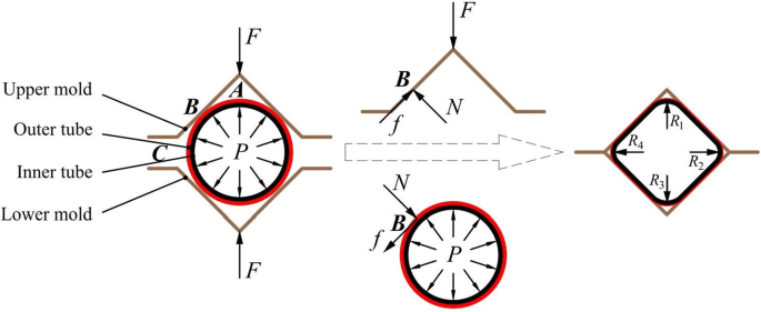
Schematic diagram of force analysis during LIF process
-
(2)
At the same mold clamping speed, the larger the mold cavity, the smaller the volume compression of the tube during mold clamping, and the less deformation of the tube, so the tube radius is larger.
-
(3)
In the same position, the fillet radius of the outer tube is always smaller than the inner tube. The reason is that the outer tube receives the mold clamping force and the reaction force of the inner tube during the LIF process, the inner tube is affected by the internal pressure in the tube and the clamping force transmitted by the outer tube, and is not in direct contact with the mold. The fillet of the inner tube depends on the fillet forming of the outer tube. Therefore, the fillet fill of the outer tube is more adequate than that of the inner tube, and the radius of the fillet is smaller.

3.3 Thickness distribution
The wall thickness distribution of the inner and outer tubes is shown in Fig. 8. Since the bulging section of the composite tube is bilaterally symmetrical, only the left part of the tube section is analyzed for wall thickness distribution in this paper. It can be found from the figure:
-
(1)
Under the clamping action of the same mold and different speed, the wall thickness distribution of each site has a good consistency, and has good symmetry along the horizontal section of the tube, this means that the clamping speed has no significant effect on the tube wall thickness forming since it only affects the ascent rate of pressure in the tube and has no effect on the total internal pressure, which is directly related to the tube wall thickness forming situation.
-
(2)
The wall thickness value at site 5 is often the largest. The reason is that during the mold clamping process, there is certain friction between the tube and the mold that affects the flow of materials, as is shown in Fig. 7. Taking point B as the boundary point, under the effect of friction, the material in the AB area is thinned by tension, and the material in the BC area is compressed and thickened, resulting in uneven distribution of the wall thickness of the tube.
-
(3)
Under the condition of different mold cavities, the inner tube has the smallest wall thickness at sites 3 and 7. When a = 31mm, the wall thickness at site 3 is t31 − i − 3 = 0.642mm and site 7 is t31 − i − 7 = 0.638mm. When a = 32mm, the wall thickness at site 3 is t32 − i − 3 = 0.643mm and site 7 is t32 − i − 7 = 0.639mm. When a = 33mm, the wall thickness at site 3 is t33 − i − 3 = 0.646mm and site 7 is t33 − i − 7 = 0.642mm. The reason is that in the early stage of mold clamping, the inner tube is affected by the internal pressure and the outer tube. The straight edge parts of the inner tube come into contact with the outer tube before the fillet parts. As the mold clamps and the internal pressure increases, fillets of the inner tube begin to fill the outer tube gradually. At this time, under the friction between the inner tube and the outer tube, the material in the middle of the straight edge flows to both ends, therefore the wall thickness at sites 3 and 7 is thin.
Fig. 8 
The effect of different mold cavities and clamping speeds on the tube wall thickness. (a) a = 31mm, outer tube, (b) a = 31mm, inner tube, (c) a = 32mm, outer tube, (d) a = 32mm, inner tube, (e) a = 33mm, outer tube, (f) a = 33mm, inner tube

4 Optimization of load parameters based on Response Surface Method
The design of experiments was carried out by Design Expert software. The mold side length A, the clamping speed B and the initial internal pressure C are selected as experimental factors, and the wall thickness variance Y1, maximum bulging height Y2 and minimum fillet radius Y3 of the formed composite tube are selected as the optimization goals. The variance of wall thickness is
Where t is the wall thickness of the tube section, \( \overline{t} \) is the average value of the wall thickness of the tube section, and N is the number of sampling points of the tube section.
The flow chart of parameter optimization based on response surface method (RSM) is shown in Fig. 9.

Flow chart of parameter optimization based on RSM
4.1 Analysis of variance (ANOVA)
The design of response surface factors and levels is shown in Table 4. A, B and C are the mold side length, clamping speed and initial internal pressure, respectively. The Box-Behnken Design (BBD) method was performed to design the experiment, and a composite tube LIF experiment plan with three factors each at three levels was established. The outer tube was analyzed first, and 17 sets of experiment plans were obtained and numerically simulated. Each experiment plan and its corresponding responses are shown in Table 5.
Considering that the influence factors of LIF are relatively complicated, it is decided to use the second-order polynomial model to fit the objective function relationship according to the tube wall thickness variance, bulging height and fillet radius. The response surface models for the fitted second-order polynomial results are shown in Equations (2), (3), and (4), which are the outer tube wall thickness variance, maximum bulging height, and minimum fillet radius, respectively.
The ANOVA was adopted to verify the significance and validity of the response surface model. The least squares method was used to fit the data to obtain the variance analysis of the outer tube wall thickness variance, maximum bulging height and minimum fillet radius. The values R2, \( {R}_{adj}^2 \), \( {R}_{pred}^2 \) of the response surface models for the three response targets are very close to 1, indicating that the established response surface model has very high credibility. The adequate precisions of the three models are all greater than 4, indicating that the model has a good resolution. The confidence level was determined to be 95%. In conclusion, the model is quite appropriate for experimental relationships between the variables and responses.
4.2 Analysis of the response surface model
To better analyze the influence of load parameters on each response target during the LIF process of composite tubes, the relationship between the optimization target and the variables was designed. Figure 10 shows a response surface analysis of the interaction effect of mold clamping speed and mold side length on the uniformity of tube wall thickness. From the response surface plot (Fig. 10 (a)), it is not difficult to find that the smaller the mold side length, the worse the uniformity of tube wall thickness distribution. It can be observed from the contour plot (Fig. 10 (b)) that the outer tube wall thickness uniformity is the best when the mold side length and the closing speed are the maxima.

Response surface analysis of uniformity of wall thickness under the interaction of mold clamping speed and mold side length (P0 = 8.567MPa). (a) 3D plot, (b) 2D plot.
Figure 11 is a response surface analysis of the interaction effect of mold clamping speed and mold side length on the maximum bulging height. It can be found that the maximum bulging height is proportional to the mold side length, and the effect of different mold clamping speeds on the bulging height is not significant. It also proves that the side length of the mold is the main parameter affecting the bulging height of the tube.

Response surface analysis of maximum bulging height under the interaction of mold clamping speed and mold side length (P0 = 8.567MPa). (a) 3D plot, (b) 2D plot.
Figure 12 is the response surface analysis of the interaction effect of mold clamping speed and mold side length on the minimum fillet radius. As the mold side length decreases, the volume compression of the tube blank cavity increases, which results in an increase in the liquid pressure in the cavity and a decrease in the radius of the tube fillet. The clamping speed has a certain effect on the minimum fillet radius. The higher the clamping speed, the smaller the minimum fillet radius. When the mold side length is the smallest (a = 31mm) and the mold clamping speed is the largest (v = 75mm/s), the tube radius reaches the minimum value. It is not difficult to find that the mold size is the main parameter that affects the minimum fillet radius of the tube, compared to clamping speed.

Response surface analysis of minimum fillet radius under the interaction of mold clamping speed and mold side length (P0 = 8.567MPa). (a) 3D plot, (b) 2D plot.
4.3 Multi-objectives optimization
The optimized loading parameters of the outer tube under the LIF environment are obtained by Design Expert, as is listed in entry 1 of Table 6, its desirability is 0.703. Similarly, the inner tube is analyzed, and the optimized loading parameters are listed as entry 2, and the desirability is 0.711. Considering that the forming quality of the inner tube can better reflect the overall forming quality of the composite tube, to unify the global loading parameters, the loading parameters of the external tube were revised, and the optimized results were shown as entry 3 in Table 6, and the response target was in line with expectations. Finally, the optimal loading parameters for the LIF of the composite tube are listed as entry 2 and entry 3, that is, the mold side length is 32.259 mm, the mold clamping speed is 25 mm/s, and the initial internal pressure is 8.567 MPa. Through the co-simulation of ANSYS Workbench and DYNAFORM, the numerical simulation results of the outer tube and the inner tube are listed as entry 4 and entry 5 in the following table. Among them, the errors of the numerical simulation results of the outer tubes’ Y1, Y2, Y3 and the response surface optimization results were 1.18%, 0.65% and 1.83%, respectively, and the errors of the numerical simulation results of the inner tubes’ Y1, Y2, Y3 and the response surface optimization results were 1.21 %, 0.56% and 1.35%, respectively.
5 Experimental verification
5.1 Experimental setup
To verify the forming characteristics of composite tubes under LIF, the YL32-200TA four-column hydraulic machine was used as the stamping equipment, the self-designed LIF apparatus was also used to perform the composite tube LIF experiment, as is shown in Fig. 13.

LIF experimental setup
According to the loading parameters optimized by RSM, the LIF experiment of the composite tube is verified, the experiment schedule was set as follows: Mold side length a=32.259mm, clamping speed v=25mm/s. The inner and outer tubes for the LIF experiment were made of SUS304 stainless steel. The geometric parameters of the tubes are shown in Table 7, the initial internal pressure P0=8.567MPa, the main mechanical properties are as follows: tensile strength σb ≥ 520MPa, yield strength σs ≥ 205MPa, elongation at break d ≥ 30%.
5.2 Results and discussions
Figure 14 shows tubes formed according to the experiment schedule, the obtained geometric parameters of the tube include the bulging height H1 and H2, the fillet radius R1, R2, R3 and R4, the wall thickness distribution t, and the dimensional schematic diagram is shown in Fig. 15.

Formed tubes in experiments

Schematic diagram of the geometric dimensions of composite tubes
5.2.1 Bulging height
Figure 16 shows the comparison of the bulging height of composite tubes formed by experiment and simulation. Since the bulging height in this paper refers to the distance between the inner walls of the tube, when composite tubes were hydroformed, there is no space to measure the bulging height of the inner wall of the outer tube, therefore, only the inner tube is involved and discussed here. It can be found from the figure that the bulging height H1 and H2 have a good consistency. The measured tube bulging height is in good agreement with the numerical simulation results, and the maximum deviation is 4.3%.

Comparison of bulging height obtained by experiment and numerical simulation
5.2.2 Fillet radius
The fillet radius at different positions of the tube are measured and shown in Fig. 17, where Ri − exp refers to the average fillet radius of the inner tube, and Ro − exp refers to the average fillet radius of the outer tube, Ri − sim refers to the fillet radius of the inner tube obtained through simulation, and Ro − sim refers to the fillet radius of the outer tube obtained through simulation. It can be found from the figure that the fillet radius R1 and R3, R2 and R4 have good consistency, and R1 and R3 are significantly larger than R2 and R4. The maximum deviation of the inner tube fillet radius is 4.13%, and the maximum deviation of the outer tube fillet radius is 4.11%, which is in line with expectations.

Comparison of fillet radius obtained by experiment and numerical simulation
5.2.3 Thickness distribution
The two layers of the tube have been formed into a whole after LIF. The micrometer is used to measure the wall thickness of the cross section of the formed composite tube. The obtained wall thickness distribution is shown in Fig. 18. It is found that the distribution of the tube wall thickness obtained by the experiment has a good consistency with the numerical simulation results. The deviation is mainly caused by the measurement error and the gap between the actual experimental conditions and the ideal conditions set by the numerical simulation. The thickest location is at site 5, and the maximum deviation occurs at site 6, which is 0.76%.

Comparison of wall thickness obtained by experiment and numerical simulation
6 Conclusions
In this paper, numerical simulation research of the forming characteristics of composite tubes under impact hydraulic load is mainly carried out. The effect of different loading parameters on the forming law of the tube is analyzed. The RSM is used to optimize the loading parameters of the tube LIF process. The optimization results were verified by LIF experiments. The conclusions can be summarized as follows:
-
(1)
Tube bulging heights H1 and H2 formed in the same mold cavity and different clamping speeds have good consistency, fillet radii R1 and R3, R2 and R4 have a good consistency. There is a clear difference between the fillet radius of the tube cross-section in the horizontal direction and vertical direction, and the wall thickness distribution has a good consistency. Tube bulging height, fillet radius, inner and outer tube spacing and wall thickness uniformity are proportional to the mold cavity.
-
(2)
The tube wall thickness variance, bulging height and fillet radius are selected as optimization targets, and the mold side length, clamping speed and initial internal pressure are selected as optimization variables to establish a response surface model with RSM. By optimizing the objective function, the optimal loading parameters are obtained. The determined optimal loading parameters are: the mold side length is 32.259mm, the mold clamping speed is 25mm/s, and the initial internal pressure is 8.567MPa.
-
(3)
Set an experiment schedule based on the loading parameters optimized by RSM. Use the LIF device to perform the experiment on composite tubes with a four-column hydraulic machine. The formed tube is of good quality, and its bulging height, fillet radius and wall thickness were in good agreement with the numerical simulation results and in line with expectations.
Availability of data and material
Not applicable
Code availability
Not applicable
References
Alaswad A, Benyounis KY, Olabi AG (2012) Tube hydroforming process: A reference guide. Mater Des 33:328–339. https://doi.org/10.1016/j.matdes.2011.07.052
Dohmann F, Hartl C (1997) Tube hydroforming - research and practical application. J Mater Process Technol 71:174–186. https://doi.org/10.1016/S0924-0136(97)00166-0
Yang J, Jeon B, Oh S (2001) Design sensitivity analysis and optimization of the hydroforming process. J Mater Process Technol 113:666–672. https://doi.org/10.1016/S0924-0136(01)00670-7
Xu XH, Zhang WG, Li SH, Lin ZQ (2009) Study of tube hydroforming in a trapezoid-sectional die. Thin-Walled Struct 47:1397–1403. https://doi.org/10.1016/j.tws.2008.12.002
Xu XH, Li SH, Zhang WG, Lin ZQ (2009) Analysis of thickness distribution of square-sectional hydroformed parts. J Mater Process Technol 209:158–164. https://doi.org/10.1016/j.jmatprotec.2008.01.034
Olabi AG, Alaswad A (2011) Experimental and finite element investigation of formability and failures in bi-layered tube hydroforming. Adv Eng Softw 42:815–820. https://doi.org/10.1016/j.advengsoft.2011.05.022
Cui XL, Wang XS, Yuan SJ (2014) Deformation analysis of double-sided tube hydroforming in square-section die. J Mater Process Technol 214:1341–1351. https://doi.org/10.1016/j.jmatprotec.2014.02.005
Cui XL, Wang XS, Yuan SJ (2015) The Bulging Behavior of Thick-Walled 6063 Aluminum Alloy Tubes Under Double-Sided Pressures. JOM 67:909–915. https://doi.org/10.1007/s11837-015-1291-1
Xie WC, Teng BG, Yuan SJ (2015) Deformation analysis of hydro-bending of bi-layered metal tubes. Int J Adv Manuf Technol 79:211–219. https://doi.org/10.1007/s00170-015-6830-y
Cui XL, Wang XS, Yuan SJ (2017) Formability improvement of 5052 aluminum alloy tube by the outer cladding tube. Int J Adv Manuf Technol 90:1617–1624. https://doi.org/10.1007/s00170-016-9488-1
Feng YY, Luo ZA, Su HL, Wu QL (2018) Research on the optimization mechanism of loading path in hydroforming process. Int J Adv Manuf Technol 94:4125–4137. https://doi.org/10.1007/s00170-017-1118-z
Feng YY, Zhang HG, Luo ZA, Wu QL (2019) Loading path optimization of T tube in hydroforming process using response surface method. Int J Adv Manuf Technol 101:1979–1995. https://doi.org/10.1007/s00170-018-3087-2
Chu GN, Sun L, Wang GD, Fan ZG, Li H (2019) Axial hydro-forging sequence for variable-diameter tube of 6063 aluminum alloy. J Mater Process Technol 272:87–99. https://doi.org/10.1016/j.jmatprotec.2019.04.038
Chu GN, Chen G, Lin CY, Fan ZG, Li H (2020) Analytical model for tube hydro-forging: Prediction of die closing force, wall thickness and contact stress. J Mater Process Technol 275:116310. https://doi.org/10.1016/j.jmatprotec.2019.116310
Ash SP (1997) Liquid impact tool forming mold. U.S. Patent. https://patents.google.com/patent/US5630334A/en
Hwang Y, Altan T (2002) FE simulations of the crushing of circular tubes into triangular cross-sections. J Mater Process Technol 125-126:833–838. https://doi.org/10.1016/S0924-0136(02)00385-0
Hwang Y, Altan T (2003) Finite element analysis of tube hydroforming processes in a rectangular die. Finite Elem Anal Des 39:1071–1082. https://doi.org/10.1016/S0168-874X(02)00157-9
Chu GN, Chen G, Lin YL, Yuan SJ (2019) Tube hydro-forging - a method to manufacture hollow component with varied cross-section perimeters. J Mater Process Technol 265:150–157. https://doi.org/10.1016/j.jmatprotec.2017.11.007
Jia YK, Li J, Luo JB (2017) Analysis and experiment on tube hydroforming in a rectangular cross-sectional die. Adv Mech Eng 9:2071938571. https://doi.org/10.1177/1687814017694831
Shahbazi Karami J, Nourbakhsh SD, Tafazzoli Aghvami K (2018) Experimental and numerical assessment of mechanical properties of thin-walled aluminum parts produced by liquid impact forming. Int J Adv Manuf Technol 96:4085–4094. https://doi.org/10.1007/s00170-018-1828-x
Zhang XL, Chu GN, He JQ, Yuan SJ (2019) Research on a hydro-pressing process of tubular parts in an open die. Int J Adv Manuf Technol 104:2795–2803. https://doi.org/10.1007/s00170-019-03893-x
Liu JW, Liu XY, Yang LF, Liang HP (2016) Investigation of tube hydroforming along with stamping of thin-walled tubes in square cross-section dies. Proc Inst Mech Eng B J Eng Manuf 230:111–119. https://doi.org/10.1177/0954405415609488
Liu JW, Yao XQ, Li YH, Liang HP, Yang LF (2019) Investigation of the generation mechanism of the internal pressure of metal thin-walled tubes based on liquid impact forming. Int J Adv Manuf Technol 105:3427–3436. https://doi.org/10.1007/s00170-019-04476-6
Funding
This study was financially supported by the National Natural Science Foundation of China (Grant No. 51765013); Guangxi Science and Technology Project (Grant No. AD19110055); and Innovation Project of GUET Graduate Education (Grant No. 2019YCXS015). The authors would like to take this opportunity to express their sincere appreciation to these funding organizations.
Author information
Authors and Affiliations
Contributions
Xinqi Yao: Conceptualization, Methodology, Investigation, Software, Validation, Writing - original draft, Writing - review & editing, Visualization. Jianwei Liu: Conceptualization, Supervision, Writing - review & editing, Project administration, Funding acquisition. Huiping Liang: Methodology. Xiangwen Fan: Resources, Investigation, Formal analysis, Data curation. Yuhan Li: Resources, Investigation, Software, Formal analysis, Validation.
Corresponding author
Ethics declarations
Conflicts of interest
The authors declare that they have no known competing financial interests or personal relationships that could have appeared to influence the work reported in this paper.
Additional information
Publisher’s note
Springer Nature remains neutral with regard to jurisdictional claims in published maps and institutional affiliations.
Rights and permissions
About this article

Cite this article
Yao, X., Liu, J., Liang, H. et al. Investigation of forming optimization of composite tubes based on liquid impact forming. Int J Adv Manuf Technol 116, 1089–1102 (2021). https://doi.org/10.1007/s00170-021-07530-4
Received:
Accepted:
Published:
Issue Date:
DOI: https://doi.org/10.1007/s00170-021-07530-4