
Abstract
The paper is concerned with the IBVP in exterior domains of the two-dimensional Stokes equations. The goal was to investigate the well-posedness in the set of solutions assuming an initial data \(u_0\in L^\infty (\Omega )\), divergence free, and enjoying the property  for all \(t>0\) and c independent of u. For all \(u_0\in L^\infty \), divergence-free one shows examples of non-uniqueness in the above set of solutions.
1 Introduction
After the articles [25, 27, 28], in the last decades, the Stokes initial boundary value problem with an initial datum in \(L^\infty \), jointly with \(L^\infty \)-estimates of the solutions, has been considered by several authors, both with homogeneous boundary data, see, e.g., [3,4,5,6, 14, 17], and with non-homogeneous; see, e.g., [7]. In the case of a two-dimensional exterior domain, apart from the contributions given in [27, 28] related to the non-homogeneous and homogeneous boundary data, respectively, based on the theory of the hydrodynamic potentials, the quoted literature, based on methods of functional analysis, achieves some results in a sequence of different papers [3, 4] and [1, 2]. Actually, the result in [3, 4] is partial, in the sense that the \(L^\infty \)-estimate a priori holds locally in time:

where the constant c and the size \(T_0\), where \(T_0\) a priori is finite, are independent of u. Subsequently in [1] estimate (1) is obtained for all \(t>0\), but the result holds paying in terms of generality. Indeed, in [1], the author considers the set of solutions for which the net force satisfies \(\int \nolimits _{\partial \Omega }\nu \cdot T(u,\pi _u)\hbox {d}\mathcal H^1=0\), where the symbol \(T(u,\pi _u)\) denotes the stress tensor and \(\nu \) is the normal to \(\partial \Omega \) . Finally, in [2], the author proves that the Stokes operator is a bounded analytic semigroup of angle \(\frac{\pi }{2}\) on the subset of \(L^\infty (\Omega )\) whose elements are divergence free, and without restriction estimate (1) holds for all \(t>0\) .
In this note, we consider the case of initial data \(u_0\in L^\infty (\Omega )\), divergence free in weak sense. If from one side our result partially solves the question, from another side, it goes beyond the question, and it brings new facts on the well-posedness problem that can be of some interest. To better introduce the last sentence, we need a short digression. In two-dimensional exterior domains, the steady boundary Stokes problem presents a “pathologic property.” One can solve the boundary value problem with a limit (say) \(a_\infty \) at infinity (\(|x|\rightarrow \infty \)), but this limit can not be given as a datum. The solution in the set of the ones assuming value \(a_\infty \) at infinity is unique (see Sect. 2 for the details). This set of solutions are else called “exceptional solutions,” see specifically, Ch. 5 Sect. 4 of [11] or also [13]. In this note, the indetermination of the quoted “boundary condition at infinity” for the steady Stokes boundary value problem becomes a key tool to prove the non uniqueness of solutions to the Stokes initial boundary value problem in exterior domains.Footnote 1
We limit ourselves to consider the two-dimensional problem, although some aspects of the construction can be considered in the n-dimensional case too.
The argument lines of the proof partially follow the ideas already employed in [17]; indeed, a new approach is considered.
In order to introduce our results, we need some notation. The symbol \(\Omega \) denotes an exterior domain of \(\mathbb R^2\) with smooth boundary \(\partial \Omega \) . We set

A field \(u\in L^\infty (\Omega )\) is said divergence free in weak sense if \(\int \nolimits _{\Omega }u\cdot \nabla \varphi \hbox {d}x=0\) for all \(\varphi \) such that \(\nabla \varphi \in L^1(\Omega )\) . As it is easy to understand, by the assumption of bounded boundary \(\partial \Omega \) and its regularity, the property of divergence free implies in particular that there exists \(u\cdot \nu \) on \(\partial \Omega \) as distribution in \(W^{-\frac{1}{p},p}(\partial \Omega )\) for all \(p\in (1,\infty )\) .
We consider the initial boundary value problem
We set
For \(R>0\), we indicate by
For the functions of one real variable, we use the Newton symbol “\(\cdot \)” to mean the derivate. We are going to prove.
Theorem 1
Let be \(R>0\) . For all \(u_0\in \mathbb L^\infty (\Omega )\) divergence free in weak sense, there exists a unique vector function \(u^\infty _R\in C^1([0,\infty ))\) and a unique solution \((u,\pi _u)\) to problem (2) such that

with \(c(R):=c\big [1+c(r)R^{-\frac{2}{r}} +c(\alpha )R^{2\alpha }\big ]\) , \(\alpha \in (0,1)\), \(r\in (2,\infty )\) and \(c, \,c(\overline{R})\) independent of \(u_0\). Moreover, for the pressure field holds:

for all
 bounded with
 . Finally, we get
 .
.
The uniqueness holds in a wider set, actually
Theorem 2
Let \((v,\pi _v)\) be a solution to problem (2) satisfying (3) and (4)\(_3\). Then solutions \((u,\pi _u)\) given in Theorem 1 and \((v,\pi _v)\) coincide up to a function of t for the pressure field.
Set \(\displaystyle M:=\min _{R\in (0,\infty )}c(R)\). Denoted by \(R_{min}\) the point of minimum of c(R) and \(u^\infty (t):=u^\infty _{R_{min}}\). We can state.
Corollary 1
Let \(u_0\in \mathbb L^\infty (\Omega )\) divergence free. Then the solution \((u,\pi _u)\) of Theorem 1 corresponding to \(R=R_{min}\) solves problem (2) and enjoys the limit property (3)\(_2\) with \(u^\infty (t)\), estimate (3)\(_3\) with \(c(R)=M\) and (3)\(_4\) and (4)\(_1\) with \(\overline{c}(R_{min})\).
We stress that the statement of the theorems, like the one of the corollary, is furnished assuming \(u_0\in \mathbb L^\infty (\Omega )\), but it also holds under the more general assumption of \(u_0\in L^\infty (\Omega )\). In this case, the essential change is related to the limit properties (3)\(_2\), that should be replaced by
where U is the unique solution to the Cauchy problem (5) below. The behavior (3)\(_4\) for  is sharp. This can be proved as in [17] (see also [14]).
-
i.
At the moment what is possible to state
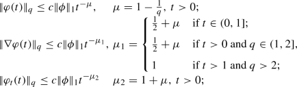
As far as we know, in the literature, the result related to the maximum modulus theorem of solutions to problem (2), which is not based on the theory of hydrodynamic potentials as made in [27, 28], is given, in n-dimensional case, \(n\ge 3\), by means of a suitable coupling of the results proved in [3] and in [17]; see also [6]. The first paper is concerned with local in time estimates and the second paper is concerned with the extension of the estimates to large time. In the two-dimensional case, the results of the first paper still work, while the results of the second paper do not work. The result in [17] is based on a technique of duality which does not work in two dimensions because, roughly speaking, the solution \(\varphi (t,x)\) of the adjoint problem has the behavior
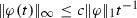 where the exponent \(-1\) is sharp. Actually, following the approach of [17], the sharp behavior allows us to deduce an estimate of the kind
  . Another result, consequence of the above arguments used in [17] is that for all ball B centered in 0,
  for all \(t>0\) and \(u_0\in L^\infty (\Omega )\) . Both the results are not suitable for the maximum modulus theorem.
Moreover, in [1, 2], the author proves that the Stokes operator is bounded and analytic on \(L^\infty (\Omega )\) whose elements are divergence free. In paper [2], estimate (1) holds for all \(t>0\).
-
ii.
The developments given in this note
In order to give a better comment to the special statement of the theorem, we firstly give an outline of the proof.
We consider a particular construction of the solution to the problem. Thank to the linear character of the equations, the solution of the theorem is seen as the sum of two solutions to problem (2): \(u:=u^1+u^2\) and \(\pi _u:=\pi _{u^1}+\pi _{u^2}\) . The solutions are derived by considering \(u_0:=u^1_0+u^2_0\). The datum \(u^1_0\) has support in \(\Omega _R\) and \(u_0^2\) has compact support in \(\overline{\Omega }-\Omega _{2R}\). We get
 with a constant c independent of R and of \(u_0\). The elements of the decomposition play a different role. As a consequence of the compact support, the solution \(u^2\) verifies the estimate
  , for all \(r\in [1,\infty )\) (see [9]). We achieve the result of maximum modulus theorem for solution \(u^2\) considering the above estimate and the results obtained (in [3, 4]) by Abe and Giga on a local interval \((0,T_0)\) (see Theorem 7). Instead, solution \(u^1\) comes by a special construction. We look for \(u^1:=U+u^\infty _R+V+W\) and \(\pi _{u^1}:=-\dot{u}^\infty _R\cdot x+\pi _U+\pi _V+\pi _W\). The fields U, V, W are solutions to the following problems:
$$\begin{aligned}&U_t-\Delta U=-\nabla \pi _U\,, \;\nabla \cdot U=0\,,\text { in }(0,T)\times \mathbb R^2,\;U=u_0^1, \text{ on } \{0\}\times \mathbb R^2, \end{aligned}$$(5)$$\begin{aligned}&\Delta V=\nabla \pi _V\,,\;\nabla \cdot V=0 \text{ in } \{t\}\!\times \!\Omega \,,\;\lim _{|x|\rightarrow \infty }\!V=0,\; V\!=-U(t)-u^\infty _R(t) \text{ on } \{t\}\times \Omega , \end{aligned}$$(6)
, for all \(r\in [1,\infty )\) (see [9]). We achieve the result of maximum modulus theorem for solution \(u^2\) considering the above estimate and the results obtained (in [3, 4]) by Abe and Giga on a local interval \((0,T_0)\) (see Theorem 7). Instead, solution \(u^1\) comes by a special construction. We look for \(u^1:=U+u^\infty _R+V+W\) and \(\pi _{u^1}:=-\dot{u}^\infty _R\cdot x+\pi _U+\pi _V+\pi _W\). The fields U, V, W are solutions to the following problems:
$$\begin{aligned}&U_t-\Delta U=-\nabla \pi _U\,, \;\nabla \cdot U=0\,,\text { in }(0,T)\times \mathbb R^2,\;U=u_0^1, \text{ on } \{0\}\times \mathbb R^2, \end{aligned}$$(5)$$\begin{aligned}&\Delta V=\nabla \pi _V\,,\;\nabla \cdot V=0 \text{ in } \{t\}\!\times \!\Omega \,,\;\lim _{|x|\rightarrow \infty }\!V=0,\; V\!=-U(t)-u^\infty _R(t) \text{ on } \{t\}\times \Omega , \end{aligned}$$(6)where we set \(\displaystyle u^\infty _R(t):=-\frac{1}{|\partial \Omega |}\int \nolimits _{\partial \Omega }U\hbox {d}\mathcal H^1\), and
$$\begin{aligned} \begin{array}{l}\displaystyle W_t-\Delta W=-\nabla \pi _W-V_t\text { in }(0,T)\times \Omega ,\quad \nabla \cdot W=0\text { in }(0,T)\times \Omega ,\\ \displaystyle W=0\text { on } (0,T)\times \partial \Omega ,\;W=0 \text{ on } \{0\}\times \Omega .\end{array}\end{aligned}$$(7)As it is known the field U is unique and the pressure field \(\pi _U\) is a function c(t). For problem (6), since the boundary data has zero integral media, we determine the existence of a unique \((V,\pi _V)\) such that
 . Moreover the regularity of U allows us to consider \(V_t(t,x)\) that we employ to determine the solution to problem (7). The solution W is special, and we refer to Sect. 4 for the details. Here we limit ourselves to stress that the support of \(u^1_0\) far from the boundary \(\partial \Omega \) implies
  . In turn it allows us to deduce, for all \(q\in (2,\infty )\),
  in a neighborhood of \(t=0\). This is one of the property that we need in order to deduce the estimates for W which are uniform in \(t>0\) with constant c(R) .
 -
iii.
The intriguing “uniqueness” of the solution
We begin saying that the uniqueness claimed by Theorem 2 has also another reading. Actually, if one is able to prove the existence of a solution \((v,\pi _v)\) enjoying the properties (3) and (4)\(_3\), then necessary this solution has a pressure field of the kind (4)\(_1\). Hence if \((v,\pi _v)\) is independent of our special construction of the solution, then (4)\(_1\) should be an a priori property of a \(L^\infty \)-solution which takes the “boundary datum” \(u^\infty _R(t)\) at infinity.
The above remark also leads to claim that no solution stated in [3, 4] can coincide with a solution of Theorem 1. In fact, denoted by \(d_\Omega (x):=dist(x,\partial \Omega )\), the set of solution \((u,\pi _u)\) considered in [3, 4] enjoys the property
 , that is conflicting with (4)\(_1\).
Although the solution \((u,\pi _u)\) is unique in the class of existence detected in Theorem 1, that is, fixed \(R>0\), u is the unique solution corresponding to \(u_0\) and assuming \(u^\infty _R(t)\), the solution is not unique with respect to \(u_0\) in the sense that varying \(R>0\), two different solutions could correspond to \(u_0\). This is a consequence of our construction. Actually, for all \(R>0\), we can determine a unique field U solution to the Cauchy problem (5) with initial datum \(u_0^1\) . Via U we define univocally \(u^\infty _R(t)\) . One could think to fix the solution \((u,\pi _u)\), with respect to \(R>0\), by requiring the best constant for the validity of estimate (3)\(_3\). Although \(\displaystyle M=\min \nolimits _{R>0}c(R)\) exists, we are not able to obtain the proof related to the sharpness of M as constant in inequality (3)\(_3\). We stress that the “anomalous” aspect of the result is independent of the fact that \(u_0\in \mathbb L^\infty (\Omega )\) . Actually, we arrive at the same result also assuming \(u_0\in C(\overline{\Omega })\). As well we stress that if \(u_0\in L^\infty (\Omega )-\mathbb L^\infty (\Omega )\) the result of existence continues to hold. The difference between the claims is in the limit property (3)\(_2\) which has to be replaced with the following:
$$\begin{aligned} \lim _{|x|\rightarrow \infty }u(t,x)-U(t)=u^\infty _R(t)\,.\end{aligned}$$In the light of the results, one understands that \(u^\infty (t)\) cannot be fixed a priori. This is the analogous of the well-posedness for the 2D-steady Stokes problem (11) in exterior domains, which plays a crucial role in our construction. Actually, for the steady problem (11) (below), without the hypothesis \(|\partial \Omega |^{-1}\int \nolimits _{\partial \Omega }a\hbox {d}\mathcal H^1=0\), one proves that the solution \((V,\pi _V)\) has the kinetic field which admits a limit \(a_\infty \) at infinity. But \(a_\infty \) cannot be a datum of the problem! Also the pair \((V,\pi _V)\) is the unique solution enjoying the limit property with value \(a_\infty \). In dimension \(n\ge 3\) one deduces the well-posedness in the \(L^\infty \)-setting, avoiding the previous indetermination, by requiring \(u^\infty (t)=0\) , for all \(t\ge 0\). We stress that \(u^\infty (t)=0\) for all \(t\ge 0\) does not means that \(\displaystyle \lim _{|x|\rightarrow \infty }u(t,x)\rightarrow 0\). Actually, the right claim is \(u(t,x)-U(t,x)\rightarrow 0\).
-
iv.
The comparison of non-uniqueness result with the examples of non-uniqueness related to problem (2)
In the paper [26], for the initial boundary value problem in the half-space (\(x_n>0\)), the well-posedness of a solution \((u,\pi _u)\) in the \(L^\infty \)-setting is achieved coupling estimate (3) for u and the request that the \(\nabla \pi _u\rightarrow 0\) for \(x_n\rightarrow \infty \). This result is doubly remarkable. One side is in connection with the example of non-uniqueness exhibited in [4]. From another side, because in the \(L^\infty \)-setting the representation formula, by means of the Green function, works for u but not for \(\pi _u\). Actually, in the paper [26], assumed \(u_0\in L^\infty (\mathbb R^n_+)\), the kinetic field \(u:=\mathbb G[u_0]\), given by means of the Green function (\(\mathbb G[\cdot ]\)), is solution because \(\frac{\partial }{\partial t}-\Delta \) on \(\mathbb G[u_0]\) matches the gradient of a function that a priori can not be represented by the formula of the pressure field because, as already said, it does not work for \(L^\infty \)-datum. As it is known, this is in contrast with the \(L^p\)-theory where the representation formula is exhaustive. Coming back to the question of uniqueness, the example given in [4] is, for \(n\ge 2\), a solution \((u,\pi _u)\) where \(u:={\underset{\small n\,\mathrm{components}}{\underbrace{(h(t,x_n),0,\cdots ,0)}}}\in L^\infty ((0,T)\times \mathbb R^n_+)\), with \(h(t,x_n)\) solution of the heat equation on the domain \((0,\infty )\times (0,\infty )\) with \(h(0,x_n)=0\) , \(h(t,0)=0\) and \(h_t-\Delta h=b(t)\), then the pressure field is \(\pi _u:=b(t)x_n\). The example of [24] (which is the first of this kind) is considered in [12] where it is extended to the case of exterior domains. The extension for the IBVP in exterior domains is given by means of the one related to the Cauchy problem, that is
$$\begin{aligned} v:=g(t)\; \text{ and } \;\pi _v:=-\dot{g}(t)\cdot x\,, \text{ with } g(0)=0\,. \end{aligned}$$All these examples of non-uniqueness, in different ways, exhibit pressure fields, for all say P(t, x), which depend on the x-space variable in a linear way and with \(\nabla P\in L^\infty (\Omega )\) for \(t>0\) (here \(\Omega \) is meant as one of the domains considered, that is the whole space or a half-space or an exterior domain). This peculiarity is crucial for the non-uniqueness. By comparing P(t, x) and the pressure field indicated in formula (4)\(_1\), one concludes that both depend on x in a linear way, and \(\nabla P\) as well \(\nabla \pi _u\in L^\infty \) for \(t>0\). It is natural to inquire why for a fixed \(R>0\) the solution of the theorem is unique. Actually, uniqueness is performed in the set of solutions which satisfy among other the limit property (3)\(_2\). This requirement is consistent as, for fixed R, the field U(t, x) and the vector function \(u^\infty _R(t)\) are uniquely determined by the initial data \(u_0\), and the limit property (3)\(_2\) for \(u_0\equiv 0\) means that \(u\rightarrow 0\) for \(|x|\rightarrow \infty \). This is not true in the case of the counterexamples. Actually, the initial data being null should give \(u^\infty _R(t)=0\) for all \(t>0\), instead, for \(t>0\), the limit is \(g(t)\ne 0\) .
-
v.
The special character of the maximum modulus theorem related to the Stokes problem
In connection with estimate (3)\(_3\), there is a discordance with the theory of Maximum Principle for parabolic and elliptic equations, or its variants for parabolic and elliptic systems. In this framework, denoted by P(u) a problem and by a the datum of the problem, the result related to the estimate (3) reads as follows:
all the solutions u of problem P(u) belonging to the class \(\mathfrak {C}\subset L^\infty \) enjoy the estimate
 (8)
(8)with the constant c which depends on the domain and on the kind of problem P(u).
So that in this statement estimate (8) becomes an a priori estimate in the set \(\mathfrak {C} \) of the solutions. In particular, for the linear character of P(u), it allows us to deduce the uniqueness in \(\mathfrak {C}\). In the light of Theorem 1, related to the case of unbounded domains, this is not possible. Of course, all this is a consequence of the further unknown of the problem, that is the pressure field, which being a dynamical variable, in particular it represents the dynamical response of the fluid, cannot be conditioned by data of the problem. From this point of view, the Stokes problem in the \(L^\infty \)-setting is conflicting with the one in the \(L^p\)-setting, where the existence of u leads to an exhaustive result concerning the continuous dependence and uniqueness of the solutions. (Actually, these solutions tend to 0 at infinity.)
 where the exponent
  . Another result, consequence of the above arguments used in [
 for all
  with a constant c independent of R and of
  , for all
  . Moreover the regularity of U allows us to consider
  . In turn it allows us to deduce, for all
  in a neighborhood of
  , that is conflicting with (
The plan of the paper is the following. In Sect. 2 we recall some estimates and results related to the \(L^p\)-theory of the steady and unsteady Stokes problem. In Sect. 3 we recall some implications that hold for the solution of Theorem 7. In Sect. 4, we furnish the first solution, that is \((u^1,\pi _{u^1})\). In Sect. 5, we furnish the second solution, that is \((u^2,\pi _{u^2})\). In Sect. 6, we conclude giving the proof of Theorems 1 and 2.
2 Some auxiliary results
In the following paper as it is usual, for \(h\in \mathbb N\), we denote by \(D^hw\) the partial derivatives of w related to a multi-index of length h. By \(\mathscr {C}_0(\Omega )\) we mean the set of function \(C_0^\infty (\Omega )\) divergence free. We denote by \(J^r(\Omega )\) and \(J^{1,r}(\Omega ),r\in (1,\infty )\,,\) the completion of \(\mathscr {C}_0(\Omega )\) in \(L^r(\Omega )\) and in \(W^{1,r}(\Omega )\), respectively.
We recall the following results.
Lemma 1
Let \(w(x)\in L^q(\Omega )\) and \(D^mw\in L^p(\Omega )\), \(p,q\in [1,\infty )\). Then, for \(k\in \{0,1,\dots ,m-1\}\), the following inequality holds

where the exponents satisfy the dimensional balance:
with \(b\in [\frac{k}{m},1]\) either if \(p=1\) or \(p>1\) and \(m-k-\frac{n}{p}\notin \mathbb N\cup \{0\}\), while \(a\in [\frac{k}{m},1)\) if \(p>1\) and \(m-k-\frac{n}{p}\in \mathbb N\cup \{0\}\) . Moreover, if D is abounded domain, then inequality (9) holds in the following form:

provided that the dimensional balance of the inequality is satisfied.
Proof
This lemma is part of an interpolation inequality proved in [8]. The difference with respect to the well known Gagliardo–Nirenberg interpolation inequality is in the fact that the value of \(D^kw\) is not zero on the boundary.\(\square \)
Lemma 2
(Bogovski’s lemma). Let \(g\in L^r(\Omega )\) with compact support and \(\int \nolimits _{\Omega }g\mathrm{d}x=0\). Then there exists a field \(G\in W_0^{1,r}(\Omega )\) with compact support such that \(\nabla \cdot G=g\) and

where \(c_P\) is the Poincaré constant and c is a constant independent of g.
Proof
See, e.g., [11].\(\square \)
We consider the boundary value problem for the Stokes system:
Theorem 3
Let \(a\in C(\partial \Omega )\) and \(|\partial \Omega |^{-1}\int \nolimits _{\partial \Omega }a(y)\mathrm{d}\sigma =0\). Then there exists a unique solution \((V,\pi _V)\) to problem (11) such that \(V\in C(\overline{\Omega })\cap C^2(\Omega )\) and \(V\in C^1(\Omega )\) with

where c is a constant independent of a. Moreover, with further hypothesis of \(a\in W^{2-\frac{1}{q},q}(\partial \Omega )\), then

where c is a constant independent of a.
Proof
Existence, uniqueness and estimate (12) can be found in [15] (Ch. 3, sect. 3) or in [21]. For similar results and regularity up to the boundary see also [11].\(\square \)
Let us consider the equation for the pressure:
We are interested to the following result:
Lemma 3
Assume that \(N\in W^{2-\frac{1}{q},q}(\partial \Omega )\). Then a solution of problem (14) is such that

where c is a constant independent of N ,
\(q>2\),
\(\alpha :=\frac{2}{q}\) ,
\(d:=\frac{q}{1+\lambda q}\) ,
\(\lambda \in (0,1-\frac{1}{q})\), and
 bounded with
 .
.
Proof
It is well known that, for solutions problem to problem (14), the following estimate holds (the estimate is due to Solonnikov in [25], and recently, it is also reproduced in [19]):

where
 , bounded, with
\(\partial (\Omega -\Omega ')\cap \partial \Omega =\emptyset \) , and seminorm
, bounded, with
\(\partial (\Omega -\Omega ')\cap \partial \Omega =\emptyset \) , and seminorm
 . For
\(\lambda =1-\frac{1}{q}\), we get the Gagliardo seminorm. For
\(q>2\) we obtain
. For
\(\lambda =1-\frac{1}{q}\), we get the Gagliardo seminorm. For
\(q>2\) we obtain

We have

Hence, we get

\(\square \)
Lemma 4
Assume that N(t, x) in Lemma 3 is a smooth one-parameter family of function in
\(W^{2-\frac{1}{q},q}(\partial \Omega )\), the time
\(t>0\) is the parameter. Assume that
 . Then, in a right neighborhood of
\(t=0\), we get
. Then, in a right neighborhood of
\(t=0\), we get

with
\(c=c(T)\) independent of N and
\(t\in (0,T)\) , exponent
\(\mu \in (0,\frac{1}{2})\), and
 bounded with
 .
.
Proof
We have to estimate the right hand side of (15). Recalling that we are studying the behavior of
 in a right neighborhood of
\(t=0\), we can limit ourselves to consider the terms with the major singularity in
\(t=0\). This is conditioned by the greater exponent for
\(t^{-1}\). Recalling that in estimate (15), we have \(a=\nabla \times N(t,x)\) and the domain \(\Omega '\) is bounded, employing the assumptions
in a right neighborhood of
\(t=0\), we can limit ourselves to consider the terms with the major singularity in
\(t=0\). This is conditioned by the greater exponent for
\(t^{-1}\). Recalling that in estimate (15), we have \(a=\nabla \times N(t,x)\) and the domain \(\Omega '\) is bounded, employing the assumptions  and
and  , then we get

with exponent \(\beta := -\frac{1}{2}(1-\frac{1}{q})(1-\frac{1}{d})(1-\alpha )-\big (\frac{1}{q}(1-\frac{1}{d})+\frac{1}{d}\big )(1-\alpha )-\alpha \). By a computation we obtain
where we recall that \(\alpha =\frac{2}{q}\), \(q>2\), \(d=\frac{q}{1+\lambda q}\) and \(\lambda \in (0,1-\frac{1}{q})\). For large q and small \(\lambda \), we arrive at \(\overline{\mu }\in (0,\frac{1}{2})\). Thus we set \(\mu -1\) as exponent in (17).\(\square \)
Lemma 5
Let \(q\in (1,\infty )\). Assume that \((v,\nabla \pi _v)\in W^{2,q}(\Omega )\cap J^{1,q}_{\ell oc}(\overline{\Omega })\times L^q(\Omega )\). Then there exists a constant c independent of \((v,\pi _v)\) such that

where  is bounded with
Proof
See, e.g., [11] or [22] .\(\square \)
We use a special formulation of problem (2), that is given \(\phi \in C_0(\Omega )\)
Due to condition (19)\(_3\), problem (19) is a weak form of the usual initial boundary value problem for the Stokes equations. This weak formulation allows us to consider initial data in the Lebesgue spaces \(L^p\) and not in the space of the hydrodynamics \(J^p\). It was introduced in [16]. Its interest is connected with the possibility of deducing estimates in \(L^r\)-Lebesgue spaces with \(r\in (1,\infty ]\) by means of duality arguments. Of course, for an initial data in \(J^p\) we come back to the classical Stokes solutions. For each \(T>0\), for \(q'\) conjugate exponent of q, we set \(W_{q'}:= \{\zeta (t,x):\zeta \in C^1([0, T]\times \overline{\Omega })\cap C(0,T;;J^{1,q'}(\Omega )) \text{ and } \zeta _t\in C([0,T];L^{q'}(\Omega ))\}\). For problem (2.1), the following result holds:
Theorem 4
Let \(\phi \in L^1(\Omega )\). Then there exists a unique solution \((\varphi ,\pi _\varphi )\) to problem (19) such that
-
i.
\(\eta>0,\,q>1,\varphi \in C(\eta ,T;J^q(\Omega ))\cap L^\infty (\eta ,T;J^{1,q}(\Omega )),\,D^2\varphi \in ,\nabla \pi _{\varphi }\in L^\infty (\eta ,T;L^q(\Omega ))\);
-
ii.
\(q\in (1,\infty ]\),
where the constant c is independent of \(\phi \) and the exponent \(\mu _1\) is sharp;
-
iii.
\(\int ^{t}_{0}\big [(\varphi (\tau ),\zeta _\tau (\tau ))-(\nabla \varphi (\tau ),\nabla \zeta (\tau ))\big ]\mathrm{d}\tau =(\varphi (t),\zeta (t))-(\phi ,\zeta (0))\), for all \(\zeta \in W_{r'}\) provided that \(\frac{1}{2}+\frac{n}{2}(1-\frac{1}{r})<1;\) finally, \(\displaystyle \lim _{t\rightarrow 0}(\varphi (t),\psi )=(\phi ,\psi )\) for all \(\psi \in \mathscr {C}_0(\Omega )\).

Remark 1
We emphasize that item iii. expresses a weak formulation just in a neighborhood of \(t=0\) that is employed for the weakness of the initial data \(\phi \). For further considerations we refer to the paper [16]. The result of Theorem 4 for the two-dimensional case is proved in [18]. It is a suitable coupling of the ones proved in [10] and those proved in [16].
In the following theorem is reproduced the classical result concerning (2), which in two-dimensional case in its complete form is proved in [9, 10]:
Theorem 5
The Stokes operator \(-P\Delta \) generates an analytic semigroup on \(J^p(\Omega ),p\in (1,\infty )\) . Moreover, for all \(\varphi _0\in J^p(\Omega ) \) and \(t>s\ge 0\) the following estimates holds:

where the constant c is independent of \(\varphi \) and the exponent \(\mu _1\) is sharp.
Proof
See [9] and [10] Theorem 1.1 and Theorem 1.2 .\(\square \)
We also need to consider
Theorem 6
For all \(f\in L^r(0,T;L^r(\Omega )),r\ge 2\) there exists a unique solution \((v,\pi _v)\) to problem (20) such that \(v\in C([0,T);J^r(\Omega ))\cap L^r(0,T;W^{2,r}(\Omega ))\) and \(\nabla \pi _v,v_t\in L^r(0,T;L^r(\Omega ))\).
Proof
See, e.g., [23] .\(\square \)
We conclude our considerations on these auxiliary results by stressing that the solutions of Theorems 3 and 6 are smooth up to the boundary if data are smooth. As well solution of Theorems 5 is smooth up to the boundary for all \(t>0\). In the next sections these properties of regularity are tacitly employed. For example, they are considered in order to achieve the regularity claimed in Theorem 1.
3 Some results obtained in [3, 4]
We recall that
Theorem 7
Let us consider the initial boundary value problem (2). Then there exists a \(T_0>0\) such that, for all \(u_0\in L^{\infty }(\Omega )\) divergence free, there exists a unique solution \((u,\pi _u)\in C^2((0,T_0\times \overline{\Omega })\times C^1((0,T_0\times \overline{\Omega })\) to the Stokes problem (2), with u(t, x) \(*\)-weakly continuous in \(t = 0\). Also the following estimates hold

where c is independent of \(u_0\).
Lemma 6
Let \(u_0\in L^\infty (\Omega )\cap L^p(\Omega )\), \(p\in (1,\infty )\). Denoted by \((u,\pi _u)\) and \((v,\pi _v)\) the solutions corresponding to \(u_0\) by virtue of Theorems 5 and 7, respectively. Then the solutions coincide up to function of t for the pressure fields.
Proof
This result is an immediate consequence of the approach employed in [3]–[4]. Hence we omit details.\(\square \)
Lemma 7
Let \((u,\pi _u)\) be the solution of Theorem 7. Set  where
where  bounded with
  , then, for some \(\mu \in (0,\frac{1}{2})\), we get

with constant c independent of \(u_0\) .
Proof
The pressure field \(\pi _u\) satisfied equation (14) with \(N:=\nabla \times u\) . By virtue of (21), we satisfy the hypotheses of Lemma 4. Hence estimate (17) holds, which proves (22). \(\square \)
4 Existence of a solution to problem (2) with a special initial datum
We are going to prove the following result:
Theorem 8
Let \(u_0\in \mathbb L^\infty (\Omega )\) divergence free in weak sense. Assume that for some \(R>0\), \(\text{ supp }\,u_0\subset \Omega _R\) . Then there exist \(u^\infty _R(t)\in C([0,T))\) with \(u^\infty _R(0)=0\) and a solution \((u,\pi _{u})\) to problem (2) such that

where we set \(u^\infty _R:=-|\partial \Omega |^{-1}\int \nolimits _{\partial \Omega }U(t,\xi )\mathrm{d}\xi \) with U solution furnished by Lemma 8, and \((u,\pi _u)\) enjoys the properties (3)–(4) and \(c_1(R):=c+c(r)\big [1+R^{-2} \big ]\), \(r\in (2,\infty )\), where the constants c and c(r) are independent of the datum of the problem. Finally, we get  .
.
We need some lemmas.
Lemma 8
Let \(u_0\) be as in Theorem 8. Then, for some \(c(t)\in C(0,T)\), there exists a unique solution (U(t, x), c(t)) to problem (5) such that, for all \(\eta >0\), U is divergence free, \(U\in C(\eta ,T;C(\mathbb R^2)\cap C^2(\mathbb R^2))\) with \(U_t\in C(\eta ,T;C(\mathbb R^2))\) and

where c is a constant independent of \(u_0\) . Finally, we also get \(U\in C([0,T);C(\mathbb R^2 -\Omega _{\frac{R}{2}}))\) with  , and \(\displaystyle \lim \nolimits _{t\rightarrow 0}\,(U(t),\psi )=(u_0,\psi )\) for all \(\psi \in \mathscr {C}_0(\mathbb R^2)\) .
Proof
We consider the solution \((U,\pi _U)\) with the kinetic field represented by means of the fundamental solution of the heat equation and the pressure field given by any continuous function \(c(t)\in C((0,T))\). Estimates (24)\(_{1,2,4}\) are well known, as well \(\lim _{t\rightarrow 0}(U(t)-u_0,\psi )=0\) for all \(\psi \in \mathscr {C}_0(\mathbb R^2)\) and the asymptotic estimates of U(t, x). For estimate (24)\(_3\) we recall that \(|x-y|\ge |y|-|x|>|y|-\frac{R}{2}>\frac{R}{2}\) for all \(x\in \mathbb R^2- \Omega _{\frac{R}{2}}\) and  . Hence, by virtue of our assumption for the initial data, we get

Hence the thesis holds. Analogously, we get the estimates for  , which completes (24)\(_3\). The above estimates also imply \(U\in C([0,T);C(\mathbb R^2-\Omega _{\frac{R}{2}}))\) . \(\square \)
Lemma 9
Let U be the solution of Lemma 8. For the vector function \(u^\infty _R(t)\) introduced in Theorem 8, we get

Proof
Estimates (25) are immediate from estimates (24).\(\square \)
Lemma 10
Assume in Theorem 3\(a:=-U(t,x)-u^\infty _R(t)\) where \(u^\infty _R(t)\) is the vector function introduced in Theorem 8. Then we get

where c is independent of a (i.e. \(u_0\)). In particular, set  , we get

where \(g_0(t)\in [0,1]\) and \(\displaystyle \lim _{t\rightarrow 0}g_0(t)=0\), \(g(t)=g_0(t)R^{-2}\) for \(t\in [0,1]\) and \(g(t)=t^{-1}\) for \(t\ge 1\).
Proof
Taking the right hand side of estimate (24)\(_3\) into account, we get  less than
  , and
, and  less then
  . Estimates (26) are consequence of (12)–(13) and (24)\(_3\). The Sobolev embedding, applied with \(q>2\), and the Poincaré inequality ensure that
  . Then
  is estimated by means of (26)\(_2\), thus we arrive at (27). \(\square \)
Lemma 11
In Theorem 3 assume \(a:=-U(t,x)-u^\infty _R(t)\) , where \(u^\infty _R(t)\) is the vector function introduced in Theorem 8. Then, \(h\in \mathbb N\), we get

with c independent of a (i.e. \(u_0\)) , and \(g(t,h)=c(h,R)g_0(t)\) for \(t\in [0,1]\) and \(g(t,h)\le t^{-h}\) for \(t\ge 1\) , where function \(g_0(t)\) is the same of the above lemma.
Proof
The first inequality is a consequence of (12) and the last inequality is deduced increasing the right hand side of (24)\(_3\) .\(\square \)
Remark 2
For the next arguments, we explicitly point out that \(g(t,1)=g(t)\).
Proof of Theorem 8
In the following we indicate by \(\overline{c}(R)\) a constant \(<\infty \), for all \(R>0\), and independent of \(u_0\), whose value is not important in the computation. We look for a solution \(u(t,x):=U(t,x)+u^\infty _R(t)+V(t,x)+W(t,x)\) and \(\pi _u(t,x):=-{\dot{u}^\infty _R}(t)\cdot x+\pi _V(t,x)+\pi _W(t,x)+c(t)\), where (U, c(t)) is the solution furnished by Lemmas 10–11. For all \(t>0\), \(u^\infty _R(t)\) is the integral media of \(-U\) on \(\partial \Omega \). By virtue of the regularity properties of U in a neighborhood of \(\partial \Omega \), we have that \(u^\infty _R(t)\) is continuous function of t, uniformly bounded in t by  , and differentiable for \(t>0\). The pair \((V,\pi _V)\) is the solution furnished by Lemma 3 and assuming boundary data \(a:=-U-u_\infty \) on \(\{t\}\times \partial \Omega \). The pair \((W,\pi _W)\) is the solution to the following problem:
where \(V_t\) is the derivate of V, hence solution to problem (11) and corresponding to the boundary data \(-U_t-{\dot{u}_\infty }\). Taking into account of estimates (28), we find \(r>2\) such that \(V_t\in L^r(0,T;L^r(\Omega )\). Hence, by virtue of Theorem 6, there exists a unique solution to problem (29), with \(W\in C([0,T;J^{1,r}(\Omega ))\cap L^r(0,T;W^{2,r}(\Omega ))\) and \(W_t,\nabla \pi _W\in L^r(0,T;L^r(\Omega ))\). By embedding, we deduce \(W\in C([0,T);C(\overline{\Omega }))\) with \(W(0,x)=0\) . Now, our aim is to find a bound of  by means of
  . For \(t>0\), we set \(\widehat{\varphi }(\tau ,x):=\varphi (t-\tau ,x)\) for all \((\tau ,x)\in (0,t)\times \Omega \), where \((\varphi ,\pi _\varphi )\) is the solution to problem (19). Taking into account Theorem 4, multiplying by \(\widehat{\varphi }\) the equation (29)\(_1\), integrating by parts on \((0,t)\times \Omega \), we get
Applying Hölder’s inequality and recalling the estimates (28) for \(V_t\), and recalling estimate ii. of Theorem 4 for \(\varphi \), we get

with \(c=c(r)\) independent of \(u_0\), \(\phi \) and t . Hence from (30) by an easy computation we deduce

Since \(\phi \) is arbitrary we arrive at

Collecting the \(L^\infty \)-estimates related to U, that is (24)\(_1\), estimate (25) for \(u^\infty _R(t)\), and (26)\(_1\) related to V, finally, estimate (32) for W(t), we complete the proof of the existence of \((u,\pi _u)\) with estimate (23). Concerning the regularity properties of \((u,\pi _u)\) they are straightforward for any term of the sum which defines our solution. Finally, we give estimates (3)\(_4\) and (4)\(_1\) . In the light of our construction of u, we consider separately any term of the sum. The behaviors of the time derivates of the terms U, \(u^\infty _R\) are immediate as well, by virtue of (28), the one for V. So we limit ourselves to consider W . In order to estimate  , we before achieve the estimates for
  , then we achieve the estimates for \(L^\infty \)-norm. Via estimates (28), for all \(r_1>2\) and \(\overline{\mu }_0\in (0,1]\), we have
  . Hence, employing Theorems 5 for \(\varphi \), we obtain

with constants which are independent of \(u_0\), \(\phi \) and t . So that via (30), by an easy computation, we deduce

where function \(G_1(t)=t\) for \(t\in [0,1]\) and \(G_1(t)=1\) for \(t\ge 1\). Since \(\phi \) is arbitrary, we arrive at

Now, we consider \(W_t\). By differentiating with respect to t the equation of W and considering the adjoint problem, integrating by parts on \((\frac{t}{2},t)\times \Omega \), we get the following:

Hence, applying Hölder’s inequality, we get

From (28) we have  and
and  , recalling ii. of Theorem 4, by virtue of (33), we obtain

Since \(\phi \) is arbitrary we easily deduce

By the same arguments employed to obtain estimate (33), we get

Via inequality (9) and estimate (18), we easily deduce that

By virtue of (28), (33), and (35), we easily arrive at

Our construction, by straightforward considerations related to U and V, furnishes also for the term  the wanted estimate, so we arrive at the proof of (3)\(_4\) . Now we are in a position to prove (4)\(_3\). Since for all \(t>0\) we get \((W,\nabla \pi _W)\in W^{2,r}\cap J^{1,r}(\Omega )\times L^r(\Omega )\), by virtue of Lemma 5, we deduce estimate (18) with \(P\Delta W:=-W_t-PV_t\). In particular, set
  , we get

Employing estimates (27) for \(\pi _V\), (28), (33) and (35) for \(V_t\), W and \(W_t\), respectively, we arrive at

Thanks to estimate (25)\(_2\) we also have  . Hence we can consider achieved (4)\(_3\). The last claims of the theorem related to the asymptotic behaviors are not difficult to prove. For the sake of the brevity, we omit the details. This completes the proof of the theorem.\(\square \)
5 Existence of a solution to problem (2) for data with compact support
For the results of the following theorem, we employ on some neighborhood of \(t=0\) the results by Abe and Giga, and then the ones typical of the \(L^q\)-theory. We are going to prove
Theorem 9
Let \(u_0\) be in (2) with compact support enclosed in \(\Omega -\Omega _{\overline{R}}\), and assume \(u_0\in L^\infty (\Omega )\) divergence free. Then there exists a unique solution \((u,\pi _u)\) to problem (2) such that, for all \(\eta ,\,T>0\), \((u,\pi _u)\in C(\eta ,T;C^2(\overline{\Omega }))\times C(\eta ,T;C^1(\overline{\Omega }))\) and

Solution \((u,\pi _u)\), with \(\pi _u\equiv \Pi _u+c(t)\), enjoys the regularity properties (3)\(_4\) and (4)\(_{2,3}\). Finally, we get  .
.
Proof
By virtue of Theorem 7 we know that there exists a solution \((u,\pi _u)\) such that, for all \(\eta ,\,T>0\), \((u,\pi _u)\in C(\eta ,T;C^2(\overline{\Omega }))\times C(\eta ,T;C^1(\overline{\Omega }))\), and there exist an interval \((0,T_0)\) and constant c, both independent of \(u_0\), such that

Finally, the limit property (37)\(_1\) holds. So that we have to complete the proof of (37)\(_2\) for all \(t\ge T_0\). Since, for all \(r>1\), \(u_0\in J^r(\Omega )\), by virtue of Theorem 5, there exists a constant c(r) such that

Since Lemma 6 holds, coupling the last estimate and (38) we complete the proof of (37)\(_2\). Estimates (3)\(_4\) for u, by virtue of Theorem 7, are true on \((0,T_0)\). In order to extend them for \(t\ge T_0\), as already made for (37), it is enough to employ the properties of the solution u in \(L^r\)-setting. Concerning \(\pi _u\) we get estimate (22) on \((0,T_0)\). Employing again the results in \(L^r\), we complete the proof of (4)\(_{2,3}\). Finally, the asymptotic property is immediate. \(\square \)
Remark 3
Without losing the generality, we can assume \(0\in \mathbb R^2-\overline{\Omega }\). Hence a possible estimate of \(|\Omega -\Omega _{\overline{R}}|^\frac{1}{q}\) is given by \(c(\overline{R}+\delta )^\frac{2}{q}\), where \(\delta :=diam (\mathbb R^2-\overline{\Omega })\).
6 Proof of the Theorems 1 and 2
6.1 Existence
Proof
We introduce a nonnegative smooth cutoff function \(h_R\) with \(h_R=1\) for \(x\in \overline{\Omega }-\Omega _R\) and \(h_R=0\) for \(x\in \overline{\Omega }_{2R}\). We denote by \(C_{R,2R}\) the compact support of \(\nabla h_R\). The following decomposition holds:
where the fields \(b^i,i=1,2,\) are the Bogovski solutions to the problems
It is known that by the Bogowski representation formula we get

and we get  , \(i=1,2\), with c independent of R and \(u_0\) . Hence \(u_0^i\in L^\infty (\Omega ),i=1,2\), is divergence free, function \(u_0^1\) has support far from \(\partial \Omega \), that is \(R=dist(\)supp
 , and trivially \(u_0^1\in L^\infty (\Omega )\cap C(\overline{\Omega }-\Omega _R)\). Instead, \(u^2_0\) has compact support. Corresponding to these data, we obtain \((u^1,\pi _{u^1})\) and \((u^2,\pi _{u^2})\) solutions to problem (2), by virtue of Theorem 8 and of Theorem 9, respectively. Setting \((u,\pi _u)\equiv (u^1+u^2,\pi _{u^1}+\pi _{u^2})\), the pair \((u,\pi _u)\) is a solution to problem (2) with an initial datum \(u_0\). The field u satisfies estimates (3)\(_3\) with constant \(c(R)=c\big [1+c(r)R^{-\frac{2}{r}} +R^{2\alpha }\big ]\) as a consequence of estimate (23) for \(u^1\) and of estimate (37) for \(u^2\), provided that one considers Remark 3. The regularity as well properties (3) and (4) are consequence of the properties of the component solutions. \(\square \)
6.2 Uniqueness
We premise the following
Lemma 12
Assume that \(u\in L^r_{\ell oc}(\overline{\Omega })\), \(r\in (1,\infty )\), \(u\rightarrow 0\) for large |x| and weakly divergence free. Assume also

where, we recall, \(\Omega _R:=\{x\in \Omega :dist(x,\partial \Omega )>R\}\). Then we get

Proof
Here \(c(R)>0\) is a constant which is independent of u and whose value is not interesting for us. We introduce a smooth non negative cutoff function \(h_R\) such that \(h_R(x)=1\) for \(|x|\le R+\varepsilon \) and \(h_R=0\) for \(|x|\ge R+1-\varepsilon \). We consider the decomposition
where we indicated by \(b_i,i=1,2,\) the Bogovski solutions to the problems
We mean that the solutions \(b_i\) are extended to 0 on \(\Omega \). Moreover, we recall that  , and by construction, the functions \(uh_R+b_1\) and \((1-h_R)u+b_2\) have weak divergence free. From the assumption (39), we get

which furnishes

here we toke the compact support of \(b_1\) into account. Since by hypothesis \((1-h_R)u+b_2\rightarrow 0\) for \(|x|\rightarrow \infty \) and by construction \((1-h_R)u+b_2=0\) on \(\partial \Omega _R\), from the last estimate we deduce

Recalling that \(h_R=1\) for \(|x|>R+1\) and \(b_2\) has compact support, the last estimate, in particular, furnishes

On the other hand we have \(u\in L^r_{\ell oc}(\bar{\Omega })\), hence in the end we obtain \(u\in J^r(\Omega )\). \(\square \)
Proof of the uniqueness
The first step is to prove that \(u-v\) belongs to \(L^r(\Omega )\) for some \(r\in (1,\infty )\). For this task we argue by duality. Let \(\varphi _0\in \mathscr {C}_0(\Omega _R)\) (that is \(dist(\partial supp,\partial \Omega )>R \)) and let \(\varphi (t,x)\) be the solution to the Cauchy problem (5) corresponding to \(\varphi _0\). It is well known that \(\varphi \) is smooth, belongs to \( L^1(\mathbb R^2)\,,\) for all \(t\ge 0\), and \(|\varphi (t,x)|\le c(\varphi _0)t^{-1} \exp [-|x|^2/8t]\) for all \(t>0\) and x such that \(dist(x,\partial \,\text{ supp }\,\varphi _0)>\frac{|x|}{2}\). Moreover, by the assumption on support of \(\varphi _0\subset \Omega _R\), we have

We set \((w,\pi _w):=(u-v,\pi _u-\pi _v)\) . Since both the kinetic fields satisfy the limit property at infinity given in (3)\(_2\), the difference \(w\rightarrow 0\) for large |x|. By virtue of (3)\(_1\) for both the pressure fields, then we have \(|\pi _w(t,x)|\le c(t)(1+|x|)\), as well for \(\pi _w\) (4)\(_3\) holds. Multiplying by \(\varphi (t-\tau ,x)\,,\,\tau \in [0,t]\) , the equation of \((w,\pi _w)\) and integrating by parts on \((s,t)\times \Omega \), we get
In the previous integration by parts we take into account that, on \((0,t)\times \Omega \), \(\varphi (t-\tau ,x)\) is a solution to the Stokes adjoint Cauchy problem. Employing estimate (41)\(_1\) related to \(\varphi \), recalling estimate (3)\(_{4}\) for  and estimate (4)\(_3\) for
  , we have that the right hand side of (42) is finite for any \(\varphi \in \mathscr {C}_0(\Omega _R)\) and \(s\ge 0\). Hence, letting \(s\rightarrow 0\), the \(*\)-weak continuity of w and properties of \(\varphi \) ensure a limit for the right-hand side with a bound, for all \(\mu \in (0,\frac{1}{2})\), of the kind

Since \(w\rightarrow 0\) for \(|x|\rightarrow \infty \), via the last estimate, by virtue of Lemma 12, we deduce

Now we consider the solution to problem (2) with an initial data \(\varphi _0\in \mathscr {C}_0(\Omega )\). Employing Theorem 5, we again denote the solution (no confusion occurs) by \((\varphi ,\pi _\varphi )\). Introduced a sequence of smooth and nonnegative cutoff functions, say \(\{\zeta ^m(x)\}\), with \(\zeta ^m=1\) for \(|x|\le m\) and \(\zeta ^m=0\) for \(|x|\ge 2m\), by virtue of Bogovski’s lemma, we can construct a sequence \(\{\varphi ^m\}\) divergence free and with compact support in \(\overline{\Omega }\) that converges to \(\varphi \) with respect to the metric \(C(0,T;J^{1,r'}(\Omega ))\cap L^r(0,T;W^{2,r'}(\Omega ))\) and with \(\{\varphi ^m_t\} \) that converges to \(\varphi _t\) with respect to the metric \(L^{r'}(0,T;L^{r'}(\Omega ))\). Multiplying equation (2) of \((w,\pi _w)\) by \(\varphi ^m(t-\tau ,x)\) and integrating by parts on \((s,t)\times \Omega \), we obtain
Letting \(m\rightarrow \infty \), we have
thus we write the formula
Recalling the \(*\)-weak continuity in t of w and estimate (43), letting \(s\rightarrow 0\) and subsequently \(m\rightarrow \infty \), we get \((w(t),\varphi _0)=0\) for all \(\varphi _0\in \mathscr {C}_0(\Omega )\). Since \(w\in J^{r}(\Omega )\) for all \(t>0\), we arrive at \(w\equiv 0\) , and from the equation \(\nabla \pi _w=0\).\(\square \)
Notes
The connection between exceptional solutions to the steady Stokes problem and some “unexpected” results for the solutions to the unsteady Stokes problem in exterior domains (\(\Omega \subset \mathbb R^n,n\ge 2\)) is present in other questions. Actually, the properties of the exceptional solutions, that we employ to distort an intuitive result of the solutions to problem (2), are also employed in the papers [22] and [20] to justify the sharpness of some time asymptotic behaviors of the solutions to problem (2): The behaviors are different from the analogous ones of the IBVP in half-space and of the Cauchy problem related to system (2).
References
Abe K., Exterior Navier-Stokes flows for bounded data, Math. Nachr. 290 (2017) 972–985. https://doi.org/10.1002/mana.201600132.
Abe K., On the large time\(L^\infty \)-estimates of the Stokes semigroup in two dimensional exterior domains, arXiv:1912.01193v1.
Abe K. and Giga Y., The\(L^\infty \)-Stokes semigroup in exterior domains, J. Evol. Equ., 14 (2014), no. 1, 1–28.
Abe K. and Giga Y., Analyticity of the Stokes semigroup in spaces of bounded functions, Acta Math. 211 (2013), no. 1, 1–46.
Abe K., Giga Y. and Hieber M., Stokes resolvent estimates in spaces of bounded functions, Ann. Sci. Éc. Norm. Supér. 48 (2015) 537–559.
Bolkart B. and Hieber M., Pointwise upper bounds for the solution of the Stokes equation on\(L^\infty _\sigma (\Omega )\)and applications, J. of Functional Analysis, 268 (2015) 1678–1710.
Chang T. and Choe H.J., Maximum modulus estimate for the solution of the Stokes equations, J. Diff. Equations, 254 (2013) 2682–2704, https://doi.org/10.1016/j.jde.2013.01.009.
Crispo F. and Maremonti P., An interpolation inequality in exterior domains, Rend. Sem. Mat. Univ. Padova 112 (2004), 11–39.
Dan W. and Shibata Y.,Remark on the\(L^q\)-\(L^\infty \)-estimate of the Stokes semigroup in a 2-dimensional exterior domain, Pacific J. Math. 189 (1999), no. 2, 223–239.
Dan W. and Shibata Y., On the\(L^q\)-\(L^r\)estimates of the Stokes semigroup in a two-dimensional exterior domain, J. Math. Soc. Japan 51 (1999), no. 1, 181–207.
Galdi G.P., An Introduction to the Mathematical Theory of the Navier-Stokes Equations, Steady-state Problems. Springer Monographs in Mathematics., Second Edition, Springer. New-York (2011).
Galdi G.P., Maremonti P. and Zhou Y., On the Navier-Stokes problem in exterior domains with non decaying initial data, J. Math. Fluid Mech. 14 (2012) 633–652.
Galdi G.P. and Simader C., Existence, uniqueness and\(L^q\)-estimates for the Stokes problem in an exterior domain, Arch. Rational Mech. Anal., 112 (1990) 291–318.
Hieber M. and Maremonti P., Bounded analyticity of the Stokes semigroup on spaces of bounded functions, Recent developments of mathematical fluid mechanics, 275–289, Adv. Math. Fluid Mech Birkhäuser/Springer., Basel, 2016.
O.A. Ladyzhenskaya, The mathematical theory of viscous incompressible flow, Gordon and Breach (1968).
Maremonti P., A remark on the Stokes problem with initial data in\(L^1\), J. Math. Fluid Mech., 13 (2011), no. 4, 469–480.
Maremonti P., On the Stokes problem in exterior domains: the maximum modulus theorem, Discrete Contin. Dyn. Syst., 34 (2014) 2135–2171, https://doi.org/10.3934/dcds.2014.34.2135.
Maremonti P., On an interpolation inequality involving the Stokes operator, 710 Contemporary Mathematics (2018) 203–209, https://doi.org/10.1090/conm/710/14371.
Maremonti P., On the\(L^p\)Helmholtz decomposition: A review of a result due to Solonnikov, Lithuanian Math. J., Vol. 58, No. 3, July, 2018, pp. 268–283, https://doi.org/10.1007/s10986-018-9403-6
Maremonti P., On the\(L^p\)-\(L^q\)estimates of the gradient of solutions to the Stokes problem, J. Evol. Equ. 19 (2019), 645–676, https://doi.org/10.1007/s00028-019-00490-z
Maremonti P., Russo R. and Starita G.,On the Stokes equations: the boundary value problem, Advances in fluid dynamics, Quad. Mat., 4 (1999) 69–140.
Maremonti P. and Solonnikov V.A., An estimate for the solutions of a Stokes system in exterior domains, (Russian) Zap. Nauchn. Sem. Leningrad. Otdel. Mat. Inst. Steklov. (LOMI) 180 (1990) 105-120, transl. in J. Math. Sci. 68 no. 2 (1994) 229–239.
Maremonti P. and Solonnikov V. A., On nonstationary Stokes problem in exterior domains, Ann. Scuola Norm. Sup. Pisa Cl. Sci. (4) 24 (1997), no. 3, 395–449.
Muratori P., Teoremi di unicità per un problema relativo alle equazioni di Navier-Stokes, Boll. Un. Mat. Ital. (4) 4 (1971) 592–613.
Solonnikov V.A., Estimates of the solutions of the nonstationary Navier-Stokes system. (Russian) Boundary value problems of mathematical physics and related questions in the theory of functions, Zap. Nauchn. Sem. Leningrad. Otdel. Mat. Inst. Steklov. (LOMI) 38 (1973), 153–231, (e.t.) J. Soviet Math., 8 (1977), 467–529.
Solonnikov V.A., On nonstationary Stokes problem and Navier-Stokes problem in a half-space with initial data nondecreasing at infinity, Function theory and applications, J. Math. Sci. (N. Y.) 114 (2003), no. 5, 1726–1740.
Solonnikov V.A., On the theory of nonstationary hydrodynamic potentials, in “The Navier-Stokes equations: theory and numerical methids”, edited by R. Salvi, 223 L.N. in Pure and applied mathematics, Marcel-Dekker (2002)
Solonnikov V.A., On the estimates of the solution of the evolution Stokes problem in weighted Hölder norms, Annali dell’Univ. di Ferrara, (Sez. VII, Sci. Mat.), 52 (2006), 137-172.
Acknowledgements
The author gives his thanks to Professor Y. Shibata for the interesting discussions on some questions concerning the maximum modulus theorem.
Funding
Open access funding provided by Università degli Studi della Campania Luigi Vanvitelli within the CRUI-CARE Agreement.
Author information
Authors and Affiliations
Corresponding author
Additional information
To Matthias Hieber on his 60th birthday.
Publisher's Note
Springer Nature remains neutral with regard to jurisdictional claims in published maps and institutional affiliations.
The research activity is performed under the auspices of GNFM-INdAM.
Rights and permissions
Open Access This article is licensed under a Creative Commons Attribution 4.0 International License, which permits use, sharing, adaptation, distribution and reproduction in any medium or format, as long as you give appropriate credit to the original author(s) and the source, provide a link to the Creative Commons licence, and indicate if changes were made. The images or other third party material in this article are included in the article’s Creative Commons licence, unless indicated otherwise in a credit line to the material. If material is not included in the article’s Creative Commons licence and your intended use is not permitted by statutory regulation or exceeds the permitted use, you will need to obtain permission directly from the copyright holder. To view a copy of this licence, visit http://creativecommons.org/licenses/by/4.0/.
About this article

Cite this article
Maremonti, P. A remark on the non-uniqueness in \(L^\infty \) of the solutions to the two-dimensional Stokes problem in exterior domains. J. Evol. Equ. 21, 3055–3077 (2021). https://doi.org/10.1007/s00028-020-00662-2
Accepted:
Published:
Issue Date:
DOI: https://doi.org/10.1007/s00028-020-00662-2