
Abstract
Android devices remain vulnerable to an increasing number of unidentified Android malware that has greatly compromised the efficacy of traditional security measures. Most classifiers are programmed to use a training process to learn from the data itself, since full expert insight to evaluate classifier parameters is difficult or impossible. This paper proposes a methodology which is a hybrid of machine learning and swarm intelligence. This methodology combines the successful exploration algorithm called the particle swarm optimization (PSO) with the extreme learning machine (ELM) classifier. ELM is a single-hidden layer feedforward neural network (FFNN) consisting of large number of hidden layer neurons, which has proved to be an excellent classifier. In this research, the optimum values of input weights and biases for the ELM classifier are determined using PSO, and it further improves the classifier’s accuracy. The dataset consists of 1700 benign and 418 malicious Android applications from which over 15,000 features of different types were extracted, and feature selection techniques were applied. The aforementioned dataset was used to experiment our proposed model, and significant results were achieved.
Access provided by Autonomous University of Puebla. Download conference paper PDF
Keywords
1 Introduction
Smartphones are ubiquitous today, serving as a portable way to enter personal data, accounts, contacts, and communication services. The Android platform has become the most dominant mobile OS since 2012. Android privacy is seriously jeopardized because of Android’s open nature due to which innumerous adware, ransomware, etc., are disguised in a large number of non-malicious apps. Given this, smartphones have been tempting victims of cyber-attacks over the years. During installation, Android device users who do not regularly check or understand app permissions allow malwares to be installed and gain access to sensitive resources, even without understanding the risk. Users’ private data, such as IMEI, SMS data, call logs, contact list, and application usage statistics, is the main target for intruders, posing a significant threat to mobile users’ confidentiality and security. Therefore, immediate measures are needed to identify and deal with malware for Android devices.
In this research article, we present a machine learning (ML)-based solution for classifying applications into benign and malware classes using an extreme learning machine (ELM) classifier whose parameters are optimized by particle swarm optimization (PSO) algorithm. We had a collection of 2118 Android applications (1700 benign + 418 malicious) as APK files [1]. We generated a dataset by unpacking these APK files into source code and extracted static information including permissions, actions, intents, services, and receivers from AndroidManifest.xml files. Using this, we created a feature set consisting of over 15,000 features. Then, we preprocessed our dataset using feature selection techniques before feeding it into the aforementioned model for classification of Android applications into benign and malicious. The explained architecture is depicted in Fig. 1.

Architecture of the proposed model
2 Related Work
Substantial research has been devoted in applying different machine learning and deep learning algorithms to classify malicious Android apps based on features which are extracted from static as well as dynamic analysis. In [2], authors have implemented a bio-inspired hybrid intelligent method for detecting Android malware (HIMDAM). This research classifies Android apps by applying extreme learning machine (ELM) as a classifier. Further, the model’s accuracy was increased by using evolving spiking neural networks (eSNNs). In this paper [3], an engine for Android malware detection (DroidDetector) based on deep learning is proposed which uses deep belief network (DBN) architecture giving 96.76% testing accuracy. A feature set consisting of 192 features was extracted using static and dynamic analysis of Android applications. This work [4] proposes DroidDeep which merges the concept of static analysis and deep learning. Firstly, more than 30,000 static features were extracted and then fed into a deep learning model based on DBN to reduce the number of features. Finally, the new feature set was put into a support vector machine (SVM) model to detect Android malware. In this paper [5], detection of probable anomalies in two malware datasets was done using a high-performance extreme learning machine (HP-ELM). The results show that this approach achieved a maximum accuracy of 95.92% for top three features. In this study [6], an efficient model is introduced which is based on feature extraction and ELM classifier to detect Android malware. This model utilizes three different feature extraction methods including independent component analysis (ICA), Karhunen–Loeve transform (KLT), and principal component analysis (PCA) and then finally compiles the results using various stacking methods. In [7], authors have proposed a fully connected deep neural network approach for malware detection resulting with maximum accuracy of 94.65%. The dataset used here consists of 331 features including information about permissions in API. This paper [8] presents an effective machine learning approach based on Bayesian classification model. The features were extracted through static analysis, and total of 58 features were selected. DroidMat [9] is a model that collects static information including API calls, required permissions, etc., from AndroidManifest.xml file and then enhances the malware detection efficiency using K-means algorithm. Singular value decomposition (SVD) was used to determine the cluster’s number, and finally, KNN algorithm was used to classify apps as benign or malicious.
3 Methodology
Static analysis for the identification of mobile malware is a fast and inexpensive approach. This method tests an application without any code execution and detects malware before the inspected application is executed. Dynamic analysis detects malware after the program under review is run or during it. Hybrid analysis consists of static as well as dynamic analysis. We are concentrating on the static analysis of mobile applications in this research.
The proposed system consists of three phases—feature extraction, feature selection and detection using machine learning models. All the phases are discussed in detail in this section.
3.1 Creating the Dataset (Feature Extraction)
We received a total of 2118 Android applications consisting of 1700 benign and 418 malicious applications [1]. The corresponding APK files were unpacked to their source code using APK tool. For static analysis, AndroidManifest.xml files were fetched. For each application, this XML file was parsed using Python 3 modules, and information related to permissions, actions, features, and receivers was gathered. These parameters would become the features of the dataset which would be used to train and test the classifier to detect malware in Android applications. Figure 2 diagrammatically represents the feature extraction process.

Feature extraction process for an Android application
In this way, after parsing all the applications, we obtained a total of 15,939 features consisting of the aforementioned parameters. Note that any feature is Boolean or binary, meaning that its feature value is 1 whenever a feature appears in an application; otherwise, it is 0.
3.2 Feature Selection
One possible solution to reduce the amount of features is to use small datasets, resulting in a smaller feature set. A second approach for reducing the number of the features is to consider a limited set of possible features, e.g. permissions for Android only. A third approach is to use methods of feature ranking and feature selection, e.g. univariate statistical tests (chi-square), evaluation of correlation-based features, information gain, gain ratio, and community-based identification and elimination of recursive features. The strength of the relationship between an individual feature and the response variable is determined by these methods. Thus, a single score indicating this relationship is obtained by each feature. Then, according to these scores, all the features in the feature vector are ranked, and the top k features are considered.
For this research, we have applied the chi-square (χ2) [10] test to find out the correlation among the features and to select the necessary features from these 15,939 features.
For a relationship with a given number of variables and sample size, the chi-square method compares the differences between the actual and the predicted results. Degrees of freedom (DOF) is considered for these experiments to determine whether, based on the cumulative number of variables and samples, a specific null hypothesis can be rejected. χ2 provides a way to assess how well a data sample fits the characteristics of the wider population the sample is supposed to represent. If the sample data does not match the population’s predicted properties that we are interested in, then we may not want to use this sample to draw conclusions about the larger population.
We apply the sklearn’s select KBest function for feature selection and use the chi-square test to evaluate the best features. We receive the scores and alpha values (p_values) for each feature. The rejection region lies when the value to alpha drops below 0.05. This indicates that the features with p_values < 0.05 are not useful for the classification of our results, and we can discard them.
After selecting the features using chi-square, we finally get a dataset with 2654 features which will be fed to the machine learning classifiers in the next phase.
3.3 Model Design
Computational models are built which are capable of generalizing a concept when a machine learning algorithm is trained with a sample of input data. In our situation, trained models generalize whether or not an application is malicious or not. Therefore, when a new unidentified dataset is used by this model, it should be able to synthesize it, understand it, and provide us a reliable result.
Firstly, we are going to split the dataset into two groups: 80% for training and 20% for testing. Next, to understand its efficiency, we will run the primitive ELM. To compare the proposed ELM with particle swarm optimization outcomes, the outcomes of the native ELM will be regarded as the gold standard [11,12,13].
3.4 Extreme Leaning Machine (ELM)
Machine learning methods have gained interest in artificial intelligence in recent years, primarily because of their contributions to various disciplines. A specific case of machine learning techniques is the extreme learning machine. ELM can be labelled as supervised learning algorithm competent of figuring out linear and nonlinear problems of classification. ELM is described by conventional artificial neural network architectures as the single layer feedforward neural network (SLFN), where it is not necessary to compute input weights and hidden layer biases iteratively [11]. An example of an ELM model is shown in Fig. 3.

ELM architecture
For each hidden neuron, let IW be (L × n) input weights and B be (L × 1) bias values and O be (C × L) output weights. In a problem with N observations for a multi-category classification (K-distinct classes) {Xi, Ti, i = 1, 2, …, N − 2, N − 1, N}, the ELM network outputs with L hidden layer neurons are identified as:-
For the jth hidden neuron, the output is Fj(.), and the corresponding activation function is F(.).
The target t is defined as
In the matrix representation, it can be written as—Y = OYl.
where Yl is an L × n matrix, which is represented as
In our case, K = 2 for binary classification. For a given number of hidden layer neurons in the ELM algorithm, the input weights (IW) and bias (B) are initialized with random values. The output weights (O) are determined analytically by considering the classifier output (Y) equal to the Boolean class label (t):
where \(Y_{l}^{ + }\) is defined as the Moore–Penrose pseudo-inverse of matrix Yl.
3.5 Optimization Technique—Particle Swarm Optimization (PSO)
PSO belongs to the group of techniques of swarm intelligence, influenced by the behavioural interactions of animals that huddle together such as ants, fireflies, and bees. It is an algorithm based on the interaction of individuals which consist of a population, in a search space to evaluate for promising regions. The action of an individual is influenced by either the best personal value achieved or the best global value achieved. Using fitness parameters just like that of evolutionary algorithms, the performance of each individual is determined. The population is called as a swarm, and particles are referred as individuals. The particles remember their best position in the past in the PSO and the optimal global position the particles have ever reached. This property lets particles search more rapidly in multidimensional space [12].
Let us consider a swarm with S number of individuals. Every Pi (i = 1, 2, …, S − 2, S − 1, S) particle in the population is defined by
-
(i)
Its current pi(k) position, referring to a probable solution to the optimization problem at iteration k;
-
(ii)
Its vi(k) velocity;
-
(iii)
The optimal Pbesti(k) position attained in its previous path.
Let Gbest(k) be the optimal global position that the particles of the swarm have found across all trajectories. Optimality of position is determined by using one or more fitness parameters specified in accordance with the optimization problem considered. The particles travel according to the following equations during the search process:
These steps are shown as a flow chart in Fig. 4. The values of constants in the above equations such as W, c1 and c2 should be calculated before the experiment for the velocity updating process. The parameters c1 and c2 denote the weighting of the terms of stochastic acceleration pulling each particle towards the positions of Pbesti and Gbest. The parameters r1 and r2 are random variables in the range of [0, 1].

Native PSO flow chart
3.6 PSO Algorithm for ELM Optimization
The following major steps need to be taken to create an ELM classifier which uses PSO to optimize its parameters. These steps are as follows:
-
1.
Randomly generate a swarm with population of S particles.
-
2.
Initialize the vectors of velocity parameter vi (i = 1, 2, 3, …, S) for each particle with random values.
-
3.
Train an ELM classifier for each particle position of the particle pi (i = 1, 2, 3, …, S), and calculate the respective accuracy/fitness function.
-
4.
Initialize the Pbesti of the particle with its starting position configuration.
-
5.
Detect Gbest representing the maximum value of the fitness function observed over all paths pursued.
-
6.
Update the velocities and the positions of the particles using the equations mentioned in the previous section.
-
7.
For every candidate particle pi, create an ELM model, train the classifier, and calculate the accuracy.
-
8.
Update the particle’s best position (Pbesti) if the current accuracy is greater than the previous attained maximum value for Pbesti.
-
9.
If maximum number of iterations have been completed, then proceed to step 10, else go to step 5.
-
10.
Select the best global value from the swarm of these particles, and use its values for input weights and biases to train the final ELM classifier which will have the best accuracy from all the models that PSO will have trained.
-
11.
Use this ELM classifier to classify applications into benign and malware classes (Fig. 5).
Fig. 5 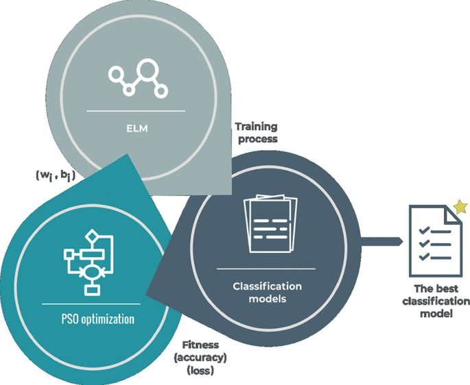
Method representation used in the proposed PSO-ELM. ELM is trained and produces a learning model. This model offers accuracy and loss, all of which are used as the fitness by the PSO algorithm to be evaluated. Finally, for the ELM, the PSO algorithm measures new weights and biases. This approach works when a stop condition is met.

4 Results
After finalizing our dataset by reducing the feature set to 2654 features using chi-square feature selection method, the proposed experimental model was divided into two major experiments.
The first experiment consisted of training a native ELM classifier using the dataset for different values of various parameters. The second experiment was the main focus of this research work. The previously developed ELM classifier was optimized using particle swarm optimization (PSO) and was trained using the same dataset for same parameter settings as the previous experiment and the results were compared.
These experiments were performed using the Python environment on a system with the specifications—Core i5-9300H @2.40 GHz with 8 GB memory.
4.1 Experiment 1
An extreme learning machine (ELM) classifier was implemented in Python using various modules like NumPy, SciPy, etc. The whole experiment was conducted twice using two activation functions—Relu and Sigmoid [13]. In each experiment, we trained a number of ELM classifiers with different number of hidden neurons starting from 100 till 1000 neurons with a step increase of 100 neurons. For a specific number of hidden neurons, ELM classifier was tested 31 times, and the mean of these accuracies was considered.
The maximum average accuracy achieved using Relu as an activation function was 93.28% at 600 neurons in hidden layer, whereas Sigmoid achieved a maximum average accuracy of 94.12% at 500 neurons in hidden layer.
4.2 Experiment 2
Particle swarm optimization (PSO) was used to improve the performance by optimizing the values of input weights and biases of ELM classifiers. This experiment was also conducted twice with the same activation functions and same iterations for the number of hidden neurons. But at each step, ELM classifier was optimized using PSO algorithm explained in Sects. 3.5 and 3.6. The parameter settings used in the PSO algorithm for this experiment are mentioned in Table 1.
The maximum accuracy achieved using Relu as an activation function was 98.58% at 600 neurons in hidden layer, whereas Sigmoid achieved a maximum accuracy of 98.82% at 400 neurons in hidden layer.
The complete results of both the experiments are described in Table 2, and their comparison is visualized in Fig. 6.

Comparison of accuracies for various classifiers with different parameters
5 Conclusion and Future Work
Malware poses a serious threat to Android applications in today’s world because data security and data privacy are of important concern to users. To tackle this problem, in this research, we came up with a modified approach to classify malicious applications from benign ones using machine learning techniques and optimized it with swarm intelligence. We extracted a total of 15,949 features which were used to create the dataset. After applying feature selection techniques, we reduced the dataset to achieve better results using our proposed model. Extreme learning machine (ELM) was used to classify the applications, which is a native method that provided us average results. Particle swarm optimization (PSO) was used to improve the performance of the classifier which gave us a maximum accuracy of 98.82% which is far superior than the traditional algorithms. The proposed idea gives us a fine-tuned model which can tackle the problem efficiently and can be of great help to expert users.
For further enhancements, we plan to upgrade this model using other machine learning and deep learning techniques and aim to optimize it further using different swarm intelligence algorithms. Work done in this research is of static analysis, and we plan to update our dataset by adding new features extracted through dynamic analysis.
References
Lashkari, A.H., Kadir, A.F.A., Taheri, L., Ghorbani, A.A.: Toward developing a systematic approach to generate benchmark android malware datasets and classification. In: Proceedings—International Carnahan Conference on Security Technology 2018-Oct 50 (2018). https://doi.org/10.1109/CCST.2018.8585560
Demertzis, K., Iliadis, L.: Bio-inspired hybrid intelligent method for detecting android malware. Adv. Intell. Syst. Comput. 416, 289–304 (2016). https://doi.org/10.1007/978-3-319-27478-2_20
Yuan, Z., Lu, Y., Xue, Y.: Droiddetector: Android malware characterization and detection using deep learning. Tsinghua Sci. Technol. 21, 114–123 (2016). https://doi.org/10.1109/TST.2016.7399288
Su, X., Zhang, D., Li, W., Zhao, K.: A deep learning approach to android malware feature learning and detection. In: Proceedings—15th IEEE International Conference on Trust, Security and Privacy in Computing and Communications, 10th IEEE International Conference on Big Data Science and Engineering and 14th IEEE International Symposium on Parallel and Distributed Processing, pp. 244–251 (2016). https://doi.org/10.1109/TrustCom.2016.0070
Shamshirband, S., Chronopoulos, A.T.: A new malware detection system using a high performance-ELM method. arXiv (2019)
Hutchison, D., Mitchell, J.C.: Advances in neural networks—ISNN 2015. In: Theoretical Computer Science, pp. 166–173 (2015). https://doi.org/10.1007/978-3-319-25393-0
Sandeep, H.R.: Static analysis of android malware detection using deep learning. In: 2019 International Conference on Intelligent Computing and Control Systems, ICCS, pp. 841–845 (2019). https://doi.org/10.1109/ICCS45141.2019.9065765
Suleiman, Y., Sezer, S., McWilliams, G., Muttik, I.: New android malware detection approach using Bayesian classification. In: Proceedings—International Conference on Advanced Information Networking and Applications, AINA, pp. 121–128. https://doi.org/10.1109/AINA.2013.88
Wu, D.J., Mao, C.H., Wei, T.E., et al.: DroidMat: android malware detection through manifest and API calls tracing. In: Proceedings of the 2012 7th Asia Joint Conference on Information Security, Asia JCIS, pp. 62–69 (2012)
Tallarida, R.J., Murray, R.B.: Chi-square test. In: Manual of Pharmacologic Calculations, pp. 140–142. Springer, New York, New York, NY (1987)
Huang, G., Zhu. Q.Y., Siew, C.K.: Extreme learning machine: theory and applications. Neurocomputing 70, 489–501 (2006). https://doi.org/10.1016/j.neucom.2005.12.126
Marini, F., Walczak, B.: Particle swarm optimization (PSO): a tutorial. Chemom. Intell. Lab. Syst. 149, 153–165 (2015). https://doi.org/10.1016/j.chemolab.2015.08.020
Ratnawati, D.E., Marjono, Widodo, Anam, S.: Comparison of activation function on extreme learning machine (ELM) performance for classifying the active compound. In: AIP Conference Proceedings, p 140001. American Institute of Physics Inc. (2020)
Author information
Authors and Affiliations
Editor information
Editors and Affiliations
Rights and permissions
Copyright information
© 2022 The Author(s), under exclusive license to Springer Nature Singapore Pte Ltd.
About this paper

Cite this paper
Gupta, R., Agarwal, A., Dua, D., Yadav, A. (2022). Android Malware Detection Using Extreme Learning Machine Optimized with Swarm Intelligence. In: Khanna, K., Estrela, V.V., Rodrigues, J.J.P.C. (eds) Cyber Security and Digital Forensics . Lecture Notes on Data Engineering and Communications Technologies, vol 73. Springer, Singapore. https://doi.org/10.1007/978-981-16-3961-6_4
Download citation
DOI: https://doi.org/10.1007/978-981-16-3961-6_4
Published:
Publisher Name: Springer, Singapore
Print ISBN: 978-981-16-3960-9
Online ISBN: 978-981-16-3961-6
eBook Packages: EngineeringEngineering (R0)