Design and Optimization of a Robust Fractional-Order FOPI Controller for Frequency Control of a Microgrid

Abstract

The paper presents the design and optimization of a fractional-order proportional integral (FOPI) controller for frequency control (FC) of a microgrid (MG) interconnecting wind, solar, and diesel-based power generation sources and a battery energy storage system (BESS). The main advantage of a FOPI controller over an integer order (IO) or classical controller is that a FOPI controller allows precise control of the phase of the input error signal in such a way that better and precise desired controller output is obtained. In this work, the value of the FO λ and controller gains has been optimized using genetic algorithm (GA)-based optimization technique. The frequency deviation of the MG using a FOPI controller has been compared with the classical IO controllers such as integral (I), PI, and PIDN controllers for both constant and random step load perturbation. Moreover, the robustness of the proposed GA–optimized FOPI controllers has been examined against random variation in wind speed and solar radiation.

1 Introduction

Since past few decades, there is more emphasis on renewable energy research including solar, wind, biomass, small hydro, geothermal, tidal, and ocean-based renewable power integration in the power system to limit the harmful effects on the environment caused due to the conventional–thermal, hydro, diesel, gas, or nuclear power generation. A microgrid (MG) is a micro-power system with multiple generating sources and storage devices. The power from an MG incorporating renewable sources depends on the availability of the source. Solar power generation depends on the intensity of solar radiation. Wind power generation depends on the speed of the wind. Fluctuations in these weather-dependent renewable power, variation in load, etc. cause frequency instability [1]. Therefore, a proper frequency control (FC) technique must be employed to tackle this issue.

The concept of fractional-order (FO) calculus was proposed hundreds of years ago, though in recent years, it has found its applications as an effective control technique in different research areas including electrical power system. The roadmap of the development of the FO controller based on the FO calculus has been discussed in research articles [2, 3]. Papers [4, 5] highlight the application of a FO controller as a FC tool. Mishra et al. [6] have used a particle swarm optimization (PSO) optimized FO proportional integral derivative (PID) controller for stabilizing the response of a nonlinear unstable system. Arya [7] and Annamraju et al. [8] have applied FO fuzzy PID controllers for FC of multi-area conventional PS. The paper [9] has utilized electric vehicle and FO controller for FC of a multi-area PS. Hence, FO controller provides a benefit of accurate and precise phase control of the input error signal by varying the FO values of λ and μ between 0 and 1. Therefore, FO can be effectively used for FC of an MG in the present problem, and also, the tuning of the fractional λ, μ values, and the gains is essential to achieve advanced frequency stability in the MG. Thus, the present paper addresses a novel application, design, and optimization of a FOPI control technique for the frequency regulation of an MG.

The flow of the present paper is as follows: The MG composition has been described in Sect. 2. The MG model has been represented in the state–space form in Sect. 3. Section 4 presents the FO control theory and the design of the proposed FOPI control scheme. Section 5 discusses the optimization methodology used for finding the optimal values of the parameters of the proposed FOPI controller. Section 6 provides the results and discussions. Finally, in Sect. 7, the conclusions from the present study have been enlisted.

2 Microgrid Composition

MG under study consists of different renewable and non-renewable sources and battery as presented in Fig. 1. The values of the MG parameters have been listed in Appendix.

Fig. 1

Microgrid model

The frequency controller can only regulate the input to conventional power sources and battery. The inputs to the wind and solar power generating sources depend solely on the weather conditions. Different generating sources and battery integrated into the MG in Fig. 1 are described below. The nonlinearities have been neglected to simplify all the transfer functions (TF).

Wind Turbine Generator System (WTGS): Input to the WTGS is input mechanical wind power, p_w which varies with the cube of the on wind speed. Hence, variation in wind speed causes variation in mechanical input power to the WTGS as well as electrical output power from the WTGS. The TF of WTGS is given by [1, 10, 11],

$$G_{{{\text{WTGS}}}} ({\text{s}}) = \frac{{K_{{{\text{WTGS}}}} }}{{1 + sT_{{{\text{WTGS}}}} }}$$

(1)

Solar Photovoltaic System (SPVS): The power output from an SPVS panel depends on solar irradiance, ϕ, and ambient temperature. The TF of SPVS is presented as [1],

$$G_{{{\text{SPVS}}}} ({\text{s}}) = \frac{{K_{{{\text{SPVS}}}} }}{{1 + sT_{{{\text{SPVS}}}} }}$$

(2)

Solar Thermal Power System (STPS): The TF of an STPS is given as [1],

$$G_{{{\text{STPS}}}} ({\text{s}}) = G_{{\text{S}}} ({\text{s}}) \cdot G_{{\text{T}}} ({\text{s}}) = \frac{{K_{{\text{S}}} }}{{1 + sT_{{\text{S}}} }} \cdot \frac{{K_{{\text{T}}} }}{{1 + sT_{{\text{T}}} }}$$

(3)

Diesel Engine Generator System (DEGS): The DEGS the only conventional energy source connected to the MG in Fig. 1. The TF of DEGS is given as [1],

$$G_{{{\text{DEGS}}}} ({\text{s}}) = \frac{{K_{{{\text{DEGS}}}} }}{{1 + sT_{{{\text{DEGS}}}} }}$$

(4)

Battery Energy Storage System (BESS): After supplying power to the loads, the surplus power generated by the MG is stored in a BESS for future usage. The TF of BESS is framed as [1],

$$G_{{{\text{BESS}}}} ({\text{s}}) = \frac{{K_{{{\text{BESS}}}} }}{{1 + sT_{{{\text{BESS}}}} }}$$

(5)

The negative sign with ΔP_BESS in Fig. 1 indicates the storing of excess power in BESS after fulfilling the load demand.

3 State–Space Representation of the Microgrid

The state–space model for MG considered in Fig. 1 has been presented in the following equations:

$$\Delta \dot{P}_{{{\text{WTGS}}}} = - \frac{1}{{T_{{{\text{WTGS}}}} }}\Delta P_{{{\text{WTGS}}}} + \frac{{K_{{{\text{WTGS}}}} }}{{T_{{{\text{WTGS}}}} }}p_{{\text{w}}}$$

(6)

$$\Delta \dot{P}_{{{\text{SPVS}}}} = - \frac{1}{{T_{{{\text{SPVS}}}} }}\Delta P_{{{\text{SPVS}}}} + \frac{{K_{{{\text{SPVS}}}} }}{{T_{{{\text{SPVS}}}} }}\phi$$

(7)

$$\Delta \dot{P}_{{{\text{ST}}}} = - \frac{1}{{T_{{\text{S}}} }}\Delta P_{{{\text{ST}}}} + \frac{{K_{{\text{S}}} }}{{T_{{\text{S}}} }}\phi$$

(8)

$$\Delta \dot{P}_{{{\text{STPS}}}} = - \frac{1}{{T_{{\text{T}}} }}\Delta P_{{{\text{STPS}}}} + \frac{{K_{{\text{T}}} }}{{T_{{\text{T}}} }}\Delta P_{{{\text{ST}}}}$$

(9)

$$\Delta \dot{P}_{{{\text{DEGS}}}} = - \frac{1}{{T_{{{\text{DEGS}}}} }}\Delta P_{{{\text{DEGS}}}} + \frac{{K_{{{\text{DEGS}}}} }}{{T_{{{\text{DEGS}}}} }}\Delta P_{c}$$

(10)

$$\Delta \dot{P}_{{{\text{BESS}}}} = - \frac{1}{{T_{{{\text{BESS}}}} }}\Delta P_{{{\text{BESS}}}} + \frac{{K_{{{\text{BESS}}}} }}{{T_{{{\text{BESS}}}} }}\Delta P_{c}$$

(11)

$$\begin{aligned} \Delta \dot{f} & = - \frac{D}{2H}\Delta f \\ & \quad + \frac{1}{2H}\left( {\Delta P_{{{\text{WTGS}}}} + \Delta P_{{{\text{SPVS}}}} + \Delta P_{{{\text{STPS}}}} + \Delta P_{{{\text{DEGS}}}} - \Delta P_{{{\text{BESS}}}} - \Delta P_{{\text{d}}} } \right) \\ \end{aligned}$$

(12)

The MG can be represented as:

$$\dot{x} = Ax + Bu + Ew$$

(13)

$$y = Cx + Du + Fw$$

(14)

where state matrix,

$$x = [\begin{array}{*{20}l} {\Delta P_{{{\text{WTGS}}}} } \hfill & {\Delta P_{{{\text{SPVS}}}} } \hfill & {\Delta P_{{{\text{ST}}}} } \hfill & {\Delta P_{{{\text{STPS}}}} } \hfill & {\Delta P_{{{\text{DEGS}}}} } \hfill & {\Delta P_{{{\text{BESS}}}} } \hfill & {\Delta f} \hfill \\ \end{array} ]^{{\text{T}}}$$

(15)

$${\text{Control}}\,{\text{input}}\,{\text{matrix}},\,u = [\Delta P_{{\text{c}}} ]$$

(16)

$${\text{Disturbance}}\,{\text{input}}\,{\text{matrix}},\,w = [\begin{array}{*{20}c} {\Delta P_{{\text{d}}} } & {p_{{\text{w}}} } & \phi \\ \end{array} ]^{{\text{T}}}$$

(17)

4 Fractional-Order PI Controller

The concept of FO calculus is based on the differintegral operator defined by Grünwald–Letnikov, Riemann–Liouville, and Caputo in their research work as mentioned in [2, 3]. In this study, a FOPI controller depicted in Fig. 2 has been used for frequency regulation of the MG shown in Fig. 1.

Fig. 2

Fractional-order (FO) controller a FO plane, b design of a FO PI controller

The TF of a classical integer-order (IO) PI controller is presented as

$$G_{{\text{C}}} \left( {\text{s}} \right) = - \left( {K_{{\text{p}}} + \frac{{K_{{\text{i}}} }}{{\text{s}}}} \right)$$

(18)

whereas the TF of a FOPI controller is denoted by,

$$G_{{\text{C}}} \left( {\text{s}} \right) = - \left( {K_{{\text{p}}} + \frac{{K_{{\text{i}}} }}{{{\text{s}}^{\lambda } }}} \right)$$

(19)

where K_p and K_i, are proportional and integral gains of the PI controller, and λ is the FO value associated with integral constant. λ can have any FO value between 0 and 1. Therefore, the most important feature of an FO controller is—by using suitable fractional value of λ, the phase angle can be controlled. Thus, FOPI controllers will minimize the error signal more efficiently than IO or classical PI controllers. Depending on the chosen value of λ which is the power of s, any phase from 0º to 90º can be deducted from the error signal resulting in a better controller output signal from the FOPI controller compared to a classical I, PI or PIDN controller.

The gains of FOPI controller and fractional-order λ value should be optimized following some boundary limits:

$$\begin{gathered} K_{{\text{p}}}^{\min } \le K_{{\text{p}}} \le K_{{\text{p}}}^{\max } \hfill \\ K_{{\text{i}}}^{\min } \le K_{{\text{i}}} \le K_{{\text{i}}}^{\max } \hfill \\ \lambda^{\min } \le \lambda \le \lambda^{\max } \hfill \\ \end{gathered}$$

(20)

The values of the boundary limits for all the parameters have been provided in Table 1. An integral time square error (ITSE)-based objective function has been used for the optimization method.

$${\text{ITSE}} = \int\limits_{0}^{t} {t\left| {\Delta f} \right|^{2} {\text{d}}t}$$

(21)

Table 1 Boundary values of the FOPI parameters

5 Optimization Method: Genetic Algorithm (GA)

GA provides reliably good optimal values of controller parameters in power system problems [12]. In GA, the no of iterations in the optimization process is called generation. There are three GA operators—selection, crossover, and mutation. The objective function is used to evaluate the fitness of the genes. The fittest chromosome is carried forward in the genes of the next generation. Tables 2 and 3 contain the GA parameters used and the optimized values of the controller parameters, respectively. The GA flowchart has been provided in Fig. 3.

Table 2 Parameters considered for GA

Table 3 Optimal values of the FOPI parameters

Fig. 3

GA flowchart

6 Results and Discussion

6.1 Comparison of FC Performance of the Proposed GA-Optimized FOPI Controller with Other Controllers

Figure 4 represents the frequency deviation curves of the MG for different classical and the proposed GA-optimized FOPI controllers for 0.1 p.u. step load change. Input to WTGS, p_w, and input to SPVS and STPS ϕ both have been taken as 0.01 p.u. (step). The auto-tunned values of the classical controller parameters have been provided in Appendix. The dynamic data corresponding to Fig. 4 has been presented in Fig. 5.

Fig. 4

Frequency response of the MG using different controllers

Fig. 5

Comparison among responses of the MG using different controllers—a undershoot, b peak undershoot time, c settling time

It has been observed from Figs. 4 and 5 that the proposed GA optimized FOPI controller provides advanced frequency regulation to the MG compared to the other IO classical controllers.

6.2 Robustness Analysis of the Proposed FOPI Controller

The performance of the proposed FOPI controller has been examined against variation in load, wind speed, and solar radiation.

• (a) Study of random variation in load: Fig. 6 depicts the frequency deviation in MG due to random load perturbation.

  Fig. 6

  

  Effect of random load on controller performance, a random load change, b frequency deviation in the MG due to random load perturbation

From Fig. 6, it has been found that the proposed FOPI controls the frequency response of the MG efficiently even during the random load perturbation in the MG.

• (b) Study of random variation in wind speed: Fig. 7 shows the frequency deviation graphs of MG against random wind speed variation.

  Fig. 7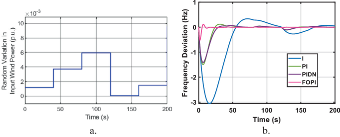

  

  Effect of random wind speed on controller performance, a random change in wind input power, b frequency deviation due to random input wind power

The input wind power, p_w, is proportional to the cube of the wind speed. Hence, a change in input mechanical power reflects a change in wind speed which results in a change in wind output electrical power as well as affects the frequency deviation. However, Fig. 7 reveals despite the random changes in WTGS input; the proposed FOPI controller regulates the MG frequency.

• (c) Study of random variation in solar radiation: Fig. 8 portrays the effect of random variation in solar radiation on frequency deviation graphs of the MG.

  Fig. 8

  

  Effect of random solar radiation on controller performance, a random change in solar radiation, b frequency deviation due to random solar radiation

Thus, Fig. 8 confirms that the random variation in solar radiation causes variation in SPVS and STPS output, but the proposed FOPI controller effectively controls the frequency of the MG under study.

7 Conclusion

An MG model comprising of WTGS, SPVS, STPS, and DEGS has been considered. A BESS has also been connected to the MG for the storage of surplus power generated by the MG. The SPVS, STPS, and WTGS power outputs depend on solar radiation and wind speed, respectively. Hence, due to the change in output power of MG caused by variation in weather conditions as well as due to some change in the disturbance, the frequency regulation is disturbed. To balance the frequency deviation, a FOPI controller has been used for FC of the MG. The FOPI controller directly controls only the input of DEGS and BESS. The optimal values of the parameters of the proposed FOPI controller have been obtained by applying the GA optimization technique. The performance of the FOPI controller has been compared with the responses for other classical controllers by applying step and random disturbances to the MG. It has been found that the non-integer type FOPI controller more efficiently regulates the frequency of the MG compared to integer type classical I, PI, and PIDN controllers in terms of settling time, peak undershoot time, and undershoot. Furthermore, the robustness of the proposed FOPI controller has been verified against change in weather conditions such as wind speed and intensity of solar radiation. Thus, it has been concluded from the simulation results that the proposed GA-optimized FOPI controller efficiently regulates the frequency of the MG.

Appendix

MG: K_WTGS = K_SPVS = K_T = 1, T_WTGS = 1.5 s, T_SPVS = 1.8 s, K_S = 1.8, T_S = 1.8 s, T_T = 0.3 s, K_DEGS = 1/300, T_DEGS = 2 s, K_BESS =  −1/300, T_BESS = 0.1 s, H = 0.083 p.u. MWs, D = 0.015 p.u. MW/Hz. I: K_i = 0.1179; PI: K_p = 3.0378, K_i = 0.5858; PIDN: K_p =  −3.5694, K_i =  −0.5374, K_d =  −1.3599, N = 18.3379.

References

R. Mandal, K. Chatterjee, Frequency control and sensitivity analysis of an isolated microgrid incorporating fuel cell and diverse distributed energy sources. Int. J. Hydrogen Energy 45(23), 13009–13024 (2020). https://doi.org/10.1016/j.ijhydene.2020.02.211
R. Matušů, Application of fractional order calculus to control theory. Int. J. Math. Model Methods Appl. Sci. 5(7), 1162–1169 (2011)
Y. Chen, I. Petras, D. Xue, Fractional Order Control—A Tutorial, American Control Conference 2009 (2009), pp. 1397–1411. https://doi.org/10.1109/ACC.2009.5160719
S. Saxena, Load frequency control strategy via fractional-order controller and reduced-order modeling. Int. J. Electr. Power Energy Syst. 104, 603–614 (2019). https://doi.org/10.1016/j.ijepes.2018.07.005
S. Das, S. Saha, S. Das, A. Gupta, On the selection of tuning methodology of FOPID controllers for the control of higher order processes. ISA Trans. 50(3), 376–388 (2011). https://doi.org/10.1016/j.isatra.2011.02.003
S.K. Mishra, D. Chandra, Stabilization and Tracking Control of Inverted Pendulum Using Fractional Order PID Controllers. J. Eng. 2014, 1–9 (2014). https://doi.org/10.1155/2014/752918
Y. Arya, AGC performance enrichment of multi-source hydrothermal gas power systems using new optimized FOFPID controller and redox flow batteries. Energy. 127, 704–715 (2017). https://doi.org/10.1016/j.energy.2017.03.129
A. Annamraju, S. Nandiraju, Robust frequency control in a renewable penetrated power system: an adaptive fractional order-fuzzy approach. Prot. Control Mod. Power Syst. 4, 1–16 (2019). https://doi.org/10.1186/s41601-019-0130-8
S. Debbarma, A. Dutta, Utilizing electric vehicles for LFC in restructured power systems using fractional order controller. IEEE Trans. Smart Grid 8(6), 2554–2564 (2016). https://doi.org/10.1109/TSG.2016.2527821
R. Mandal, K. Chatterjee, B.K. Patil, Load frequency control of a single area hybrid power system by using integral and LQR based integral controllers, in 20th National Power Systems Conference (NPSC) 2018 (IEEE, 2018), pp. 1–6. https://doi.org/10.1109/NPSC.2018.8771727
D. Bhagdev, R. Mandal, K. Chatterjee, Study and application of MPC for AGC of two area interconnected thermal-hydro-wind system, in Innovations in Power and Advanced Computing Technology (i-PACT) 2019I(EEE, 2019), pp. 1–6. https://doi.org/10.1109/i-PACT44901.2019.8960124
X. Lü, Y. Wu, J. Lian, Y. Zhang, C. Chen, P. Wang, L. Meng, Energy management of hybrid electric vehicles: a review of energy optimization of fuel cell hybrid power system based on genetic algorithm. Energy Convers. Manag. 205, 112474 (2020). https://doi.org/10.1016/j.enconman.2020.112474
Author information
Authors and Affiliations
Corresponding author
Editor information
Editors and Affiliations