Spectral Analysis of Signals

Abstract

The process of determining the frequency contents of a continuous-time signal in the discrete-time domain is known as spectral analysis. Most of the phenomena that occur in nature can be characterized statistically by random processes. Hence, the main objective of spectral analysis is the determination of the power spectrum density (PSD) of a random process. The power is the Fourier transform of the autocorrelation sequence of a stationary random process. The PSD is a function that plays a fundamental role in the analysis of stationary random processes in that it quantifies the distribution of the total power as a function of frequency. The power spectrum also plays an important role in detection, tracking, and classification of periodic or narrowband processes buried in noise. Other applications of spectrum estimation include harmonic analysis and prediction, time series extrapolation and interpolation, spectral smoothing, bandwidth compression, beam forming, and direction finding. The estimation of the PSD is based on a set of observed data samples from the process. Estimating the power spectrum is equivalent to estimating the autocorrelation. This chapter deals with the nonparametric methods, parametric methods, and subspace methods for power spectrum estimation. Further, the spectrogram computation of non-stationary signals using STFT is also briefly discussed in this chapter.

These keywords were added by machine and not by the authors. This process is experimental and the keywords may be updated as the learning algorithm improves.

The process of determining the frequency contents of a continuous-time signal in the discrete-time domain is known as spectral analysis. Most of the phenomena that occur in nature can be characterized statistically by random processes. Hence, the main objective of spectral analysis is the determination of the power spectrum density (PSD) of a random process. The power is the Fourier transform of the autocorrelation sequence of a stationary random process. The PSD is a function that plays a fundamental role in the analysis of stationary random processes in that it quantifies the distribution of the total power as a function of frequency. The power spectrum also plays an important role in detection, tracking, and classification of periodic or narrowband processes buried in noise. Other applications of spectrum estimation include harmonic analysis and prediction, time series extrapolation and interpolation, spectral smoothing, bandwidth compression, beam forming, and direction finding. The estimation of the PSD is based on a set of observed data samples from the process. Estimating the power spectrum is equivalent to estimating the autocorrelation. This chapter deals with the nonparametric methods, parametric methods, and subspace methods for power spectrum estimation. Further, the spectrogram computation of non-stationary signals using STFT is also briefly discussed in this chapter.

12.1 Nonparametric Methods for Power Spectrum Estimation

Classical spectrum estimators do not assume any specific parametric model for the PSD. They are based solely on the estimate of the autocorrelation sequence of the random process from the observed data and hence work in all possible situations, although they do not provide high resolution. In practice, one cannot obtain unlimited data record due to constraints on the data collection process or due to the necessity that the data must be WSS over that particular duration.

When the method for PSD estimation is not based on any assumptions about the generation of the observed samples other than wide-sense stationary, then it is termed a nonparametric estimator.

12.1.1 Periodogram

The periodogram was introduced in [1] searching for hidden periodicities while studying sunspot data. There are two distinct methods to compute the periodogram. One approach is the indirect method. In this approach, first we determine the autocorrelation sequence $r(k)$ from the data sequence x(n) for $- (N - 1) \le k \le (N - 1)$ and then take the DTFT, i.e.,

$$ \hat{P}_{\text{PER}} (f) = \sum\limits_{k = - N + 1}^{N - 1} {\hat{r}[k]{\text{e}}^{ - j2\pi fk} } . $$

(12.1)

It is more convenient to write the periodogram directly in terms of the observed samples x[n]. It is then defined as

$$ \hat{P}_{\text{PER}} \left( f \right) = \frac{1}{N}\left| {\sum\limits_{n = 0}^{N - 1} {x[n]{\text{e}}^{ - j2\pi fn} } } \right|^{2} = \frac{1}{N}\left| {X\left( f \right)} \right|^{2} $$

(12.2)

where $X\left( f \right)$ is the Fourier transform of the sequence x(n). Thus, the periodogram is proportional to the squared magnitude of the DTFT of the observed data. In practice, the periodogram is calculated by applying the FFT, which computes it at a discrete set of frequencies.

$$ D_{f} = \left\{ {f_{k} :f_{k} = \frac{k}{N},\quad k = 0,1,2, \ldots ,\left( {N - 1} \right)} \right\} $$

The periodogram is then expressed by

$$ \hat{P}_{\text{PER}} \left( {f_{k} } \right) = \frac{1}{N}\left| {\sum\limits_{n = 0}^{N - 1} {x[n]{\text{e}}^{ - j2\pi kn/N} } } \right|^{2} \quad f_{k} \in D_{f} . $$

(12.3)

To allow for finer frequency spacing in the computed periodogram, we define a zero-padded sequence according to

$$ x^{\prime}[n] = \left\{ {\begin{array}{*{20}l} {x[n],} \hfill & {n = 0,1, \ldots ,N - 1} \hfill \\ {0,} \hfill & {n = N,N + 1, \ldots ,N^{\prime}} \hfill \\ \end{array} } \right.. $$

(12.4)

Then we specify the new set of frequencies $D^{\prime}_{f} = \{ f_{k} :f_{k} = k/N,k \in \{ 0,1,2, \ldots ,(N - 1)\} \} ,$ and obtain

$$ \hat{P}_{\text{PER}} \left( {f_{k} } \right) = \frac{1}{N}\left| {\sum\limits_{n = 0}^{N - 1} {x[n]{\text{e}}^{{ - j2\pi kn/N^{\prime}}} } } \right|^{2} \quad f_{k} \in D^{\prime}_{f} . $$

(12.5)

A general property of good estimators is that they yield better estimates when the number of observed data samples increases. Theoretically, if the number of data samples tends to infinity, the estimates should converge to the true values of the estimated parameters. So, in the case of a PSD estimator, as we get more and more data samples, it is desirable that the estimated PSD tends to the true value of the PSD. In other words, if for finite number of data samples the estimator is biased, the bias should tend to zero as N $\to \infty$ as should the variance of the estimate. If this is indeed the case, the estimator is called consistent. Although the periodogram is asymptotically unbiased, it can be shown that it is not a consistent estimator. For example, if {$\tilde{X}$[n]} is real zero mean white Gaussian noise, which is a process whose random variables are independent, Gaussian, and identically distributed with variance $\sigma^{2}$, the variance of $\hat{P}_{\text{PER}} \left( f \right)$ is equal to $\sigma^{4}$ regardless of the length N of the observed data sequence. The performance of the periodogram does not improve as N gets larger because as N increases, so does the number of parameters that are estimated, P$\left( {f_{0} } \right)$, P$\left( {f_{1} } \right)$, …, P$\left( {f_{N - 1} } \right)$. In general, the variance of the periodogram at any given frequency is

$$ \begin{aligned} {\text{Var}}\left[ {\widehat{P}_{\text{PER}} \left( f \right)} \right] & = {\text{Cov}}\left[ {\widehat{P}_{\text{PER}} \left( f \right),\widehat{P}_{\text{PER}} \left( f \right)} \right] \\ & = P^{2} \left( f \right)\left[ {1 + \left( {\frac{\sin 2\pi Nf}{N\sin 2\pi f}} \right)^{2} } \right] \\ \end{aligned} $$

(12.6a)

For frequencies not near 0 or 1/2, the above equation reduces to

$$ {\text{Var}}(\hat{P}_{\text{PER}} \left( f \right)) \cong P^{2} \left( f \right) $$

(12.6b)

where P²(f) is the periodogram spectral estimation based on the definition of PSD.

Example 12.1

Consider a random signal composed of two sinusoidal components of frequencies 120 and 280 Hz corrupted with Gaussian distributed random noise. Evaluate its power spectrum using periodogram. Assume sampling frequency F_s = 1024 Hz.

Solution

The following MATLAB program can be used to evaluate the power spectrum of the considered signal using Bartlett’s method.

%Program 12.1

• Power spectrum estimation using the periodogram

• clear;clc;

• N = 512;%total number of samples

• k = 0:N-1;

• f1 = 120;

• f2 = 280;

• F_T = 1024;%sampling frequency in Hz

• T = 1/F_T;

• x = sin(2*pi*f1*k*T) + sin(2*pi*f2*k*T)+2*randn(size(k));%vector of length N

• %containing input samples

• [pxx,f] = psd(x,length(x),F_T);

• plot(f,pxx);grid;

• xlabel('Frequency(Hz)');ylabel('Power spectrum');

• The power spectrum obtained from the above MATLAB program is shown in Fig. 12.1.

  Fig. 12.1

  

  Power spectrum estimation using the periodogram

12.1.2 Bartlett Method

In the Bartlett method [2], the observed data is segmented into $K$ non-overlapping segments and the periodogram of each segment is computed. Finally, the average of periodogram of all the segments is evaluated. The Bartlett estimator has a variance that is smaller than the variance of the periodogram.

Consider a length N sequence x(n). Then, x(n) can be segmented into K subsequence, each subsequence having a length L. If the ith subsequence is denoted by $x_{i} (n)$, $0 \le i < K,$ then the ith subsequence can be obtained from the sequence x(n) as

$$ x_{i} (n) = x(iL + n),\quad 0 \le n \le L - 1 $$

and its periodogram is given by

$$ \overset{\lower0.5em\hbox{$\smash{\scriptscriptstyle\frown}$}}{P}_{i} \left( f \right) = \frac{1}{L}\left| {\sum\limits_{n = 0}^{L - 1} {x_{i} (n){\text{e}}^{ - j2\pi fn} } } \right|^{2} \quad i = 0,1, \ldots ,K - 1 $$

(12.7)

Then the Bartlett spectrum estimator is

$$ \widehat{P}_{\text{B}} \left( f \right) = \frac{1}{K}\sum\limits_{i = 1}^{K} {\widehat{{P_{i} }}} \left( f \right) $$

(12.8)

$$ {\text{Var}}\left( {\widehat{P}_{\text{B}} \left( f \right)} \right) = \frac{1}{K}P^{2} \left( f \right). $$

(12.9)

The variance of the Barlett estimator can be related to the variance of the periodogram as follows.

The Bartlett estimator variance is reduced by a factor of K compared to the variance of the periodogram. However, the reduction in the variance is achieved at the cost of decrease in resolution. Thus, this estimator allows for a trade-off between resolution and variance.

The following example illustrates the computation of the power spectrum of a random signal using the Bartlett method.

Example 12.2

Consider the random signal of Example 12.1 and evaluate its power spectrum using Bartlett’s method.

Solution

The following MATLAB program can be used to evaluate the power spectrum of the considered signal using Bartlett’s method.

%Program 12.2

• Power spectrum estimation using Bartlett’s method

• clear;clc;

• N = 512;%total number of samples

• k = 0 : N-1;

• f1 = 120;

• f2 = 280;

• F_T = 1024;%sampling frequency in Hz

• T = 1/F_T;

• x = sin(2*pi*f1*k*T) + sin(2*pi*f2*k*T)+2*randn(size(k));%vector of length N

• %containing input samples

• L = 128;%length of subsequence

• [pxx,f] = psd(x,L,F_T);

• plot(f,pxx);grid;

• xlabel('Frequency(Hz)');ylabel('Power spectrum');

• The power spectrum obtained from the above MATLAB program is shown in Fig. 12.2.

  Fig. 12.2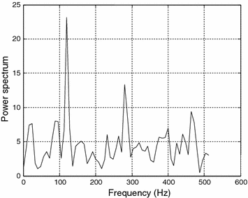

  

  Power spectrum estimation using Bartlett’s method

12.1.2.1 Welch Method

The Welch method [3] is another estimator that exploits the periodogram. It is based on the same idea as the Bartlett’s approach of splitting the data into segments and finding the average of their periodogram. The difference is that the segments are overlapped, and the data within a segment is windowed. If a sequence x(n) of length N is segmented into K subsequences, each subsequence having a length L with an overlapping of D samples between the adjacent subsequences, then

$$ N = L + D(K - 1) $$

(12.10)

where N is the total number of observed samples and K the total number of subsequences. Note that if there is no overlap, K = N/L, and if there is 50% overlap, K = 2 N/L – 1.

The ith subsequence is defined by

$$ x_{i} (n) = x(n + iD), \quad 0 \le n \le L - 1;0 \le i \le K - 1, $$

(12.11)

and its periodogram is given by

$$ \hat{P}_{i} \left( f \right) = \frac{1}{L}\left| {\sum\limits_{n = 0}^{L - 1} {w(n)x_{i} (n){\text{e}}^{ - j2\pi fn} } } \right|^{2} . $$

(12.12)

Here $\hat{P}_{i} (f)$ is the modified periodogram of the data because the samples x(n) are weighted by a non-rectangular window $w(n)$; the Welch spectrum estimate is then given by

$$ \widehat{P}_{\text{Wel}} \left( f \right) = \frac{1}{KC}\mathop \sum \limits_{i = 1}^{K} \widehat{P}_{i} \left( f \right) $$

(12.13)

where C is the normalization factor for power in the window function given by

$$ C = \frac{1}{K}\mathop \sum \limits_{n = 0}^{K - 1} w^{2} \left( n \right) $$

Welch has shown that the variance of the estimator is

$$ {\text{Var}}\left( {\widehat{P}_{\text{Wel}} \left( f \right)} \right) \approx \frac{1}{K}P^{2} \left( f \right)\quad \text{for no overlapping} $$

(12.14a)

$$ \approx \frac{9}{8K}P^{2} \left( f \right)\quad {\text{for}}\;50\% \;{\text{overlapping}}\;{\text{and}}\;{\text{Bartlett}}\;{\text{window}} . $$

(12.14b)

By allowing overlap of subsequences, more number of subsequences can be formed than in the case of Bartlett’s method. Consequently, the periodogram evaluated using the Welch’s method will have less variance than the periodogram evaluated using the Bartlett method.

Example 12.3

Consider the random signal of Example 12.1 and evaluate its power spectrum using Welch’s method with 50% overlapping and Hamming window.

Solution

The following MATLAB program can be used to evaluate the power spectrum of the considered signal using Welch’s method.

%Program 12.3

• Power spectrum estimation using Welch’s method

• clear;clc;

• N = 512;%total number of samples

• k = 0 : N-1;

• f1 = 120;

• f2 = 280;

• F_T = 1024;%sampling frequency in Hz

• T = 1/F_T;

• x = sin(2*pi*f1*k*T) + sin(2*pi*f2*k*T)+2*randn(size(k));%vector of length N

• %containing input samples

• L = 128;%length of subsequence

• window = hamming(L);% window type

• overlap = L/2;%number of overlapping samples(50%overlapping)

• [pxx,f] = psd(x,L,F_T,window,overlap);

• plot(f,pxx);grid;

• xlabel('Frequency(Hz)');ylabel('Power spectrum');

• The power spectrum obtained from the above MATLAB program is shown in Fig. 12.3.

  Fig. 12.3

  

  Power spectrum estimation using Welch’s method

12.1.2.2 Blackman–Tukey Method

In this method, autocorrelation of the observed data sequence x(n) is computed first. Next, the autocorrelation is windowed and then the Fourier transform is applied on it to obtain the power spectrum. Hence, the power spectrum using the Blackman–Tukey method [4] is given by

$$ \widehat{P}\left( f \right) = \sum\limits_{{k = - \left( {N - 1} \right)}}^{N - 1} {w\left( k \right)\widehat{r}\left( k \right){\text{e}}^{ - j2\pi fk} } $$

(12.15)

where the window $w(k)$ is real nonnegative, symmetric, and non-increasing with $\left| k \right|$, that is,

$$ ({\text{i}})\quad 0 \le w(k) \le w(0) = 1 $$

(12.16a)

$$ ({\text{ii}})\quad w( - k) = w(k) $$

(12.16b)

$$ ({\text{iii}})\quad w(k) = 0.M < \left| k \right|.\quad M \le N - 1. $$

(12.16c)

It should be noted that the symmetry property of $w(k)$ ensures that the spectrum is real. It is obvious that the autocorrelation with smaller lags will be estimated more accurately than the ones with lags close to N because of the different number of terms that are used. Therefore, the large variance of the periodogram can be ascribed to the large weight given to the poor autocorrelation estimates used in its evaluation. Blackman and Tukey proposed to weight the autocorrelation sequence so that the autocorrelations with higher lags are weighted less. The bias, the variance, and the resolution of the Blackman–Tukey method depend on the applied window. For example, if the window is triangular (Bartlett),

$$ w_{\text{B}} [k] = \left\{ {\begin{array}{*{20}l} {\frac{M - \left| k \right|}{M},} \hfill & {\left| k \right| \le M} \hfill \\ {0,} \hfill & {\text{otherwise}} \hfill \\ \end{array} } \right. $$

(12.17)

and if $N \gg M \gg 1$, the variance of the Blackman–Tukey estimator is

$$ {\text{Var}}(\hat{P}_{\text{BT}} \left( f \right)) \cong \frac{2M}{3N}P^{2} \left( f \right) $$

(12.18)

where P(f) is the true spectrum of the process. Compared to Eqs. (12.6a) and (12.6b) it is clear that the variance of this estimator may be significantly smaller than the variance of the periodogram. However, as M decreases, so does the resolution of the Blackman–Tukey estimator.

Example 12.4

Consider the random signal of Example 12.1 and evaluate its power spectrum using Blackman–Tukey method.

Solution

The following MATLAB program can be used to evaluate the power spectrum of the considered signal using Blackman–Tukey method.

%Program 12.4

• Power spectrum estimation Blackman–Tukey method

• clear;clc;

• N = 512;%total number of samples

• k = 0 : N-1;

• f1 = 120;

• f2 = 280;

• F_T = 1024;%sampling frequency in Hz

• T = 1/F_T;

• x = sin(2*pi*f1*k*T)+sin(2*pi*f2*k*T)+2*randn(size(k));%vector of length N

• %containing input samples

• r = f_corr(x,x,0,0);% evaluates correlation of input samples

• L = 128;%length of window

• window = Bartlett(L);% window type

• [pxx,f] = psd(r,L,F_T,window);

• plot(f,pxx);grid

• xlabel('Frequency(Hz)');ylabel('Power spectrum(dB)');

• The power spectrum obtained from the above MATLAB program is shown in Fig. 12.4.

  Fig. 12.4

  

  Power spectrum estimation using Blackman–Tukey method

12.1.3 Performance Comparison of the Nonparametric Methods

The performance of a PSD estimator is evaluated by quality factor. The quality factor is defined as the ratio of the squared mean of the PSD to the variance of the PSD given by

$$ Q_{P} = \frac{{\text{var} (\hat{p}(f))}}{{E^{2} (\hat{p}(f))}}. $$

(12.19)

Another important metric for comparison is the resolution of the PSD estimators. It corresponds to the ability of the estimator to provide the fine details of the PSD of the random process. For example, if the PSD of the random process has two peaks at frequencies $f_{1}$ and $f_{2}$, then the resolution of the estimator would be measured by the minimum separation of $f_{1}$ and $f_{2}$ for which the estimator still reproduces two peaks at $f_{1}$ and $f_{2}$. It has been shown in [5] for triangular window that the quality factors of the classical methods are as shown in Table 12.1.

Table 12.1 Comparison of performance of classical methods

From the above table, it can be observed that the quality factor is dependent on the product of the data length N and the frequency resolution $\Delta f$. For a desired quality factor, the frequency resolution can be increased or decreased by varying the data length N.

12.2 Parametric or Model-Based Methods for Power Spectrum Estimation

The classical methods require long data records to obtain the necessary frequency resolution. They suffer from spectral leakage effects, which often mask weak signals that are present in the data which occur due to windowing. For short data lengths, the spectral leakage limits frequency resolution.

In this section, we deal with power spectrum estimation methods in which extrapolation is possible if we have a priori information on how data is generated. In such a case, a model for the signal generation can be constructed with a number of parameters that can be estimated from the observed data. Then, from the estimated model parameters, we can compute the power density spectrum.

Due to modeling approach, we can eliminate the window function and the assumption that autocorrelation sequence is zero outside the window. Hence, these have better frequency resolutions and avoid problem of leakage. This is especially true in applications where short data records are available due to time variant or transient phenomena.

The parametric methods considered in this section are based on modeling the data sequence $y\left( n \right)$ as the output of a linear system characterized by a rational system function of the form

$$ \user2 {H\left( Z \right)} = \user2{\frac {B\left( Z \right)}{A\left( Z \right)}} = \user2{\frac{{\sum\nolimits_{k = 0}^{q} {b_{k} z^{ - k} } }}{{1 + \sum\nolimits_{k = 1}^{p} {a_{k} z^{ - k} } }}}. $$

(12.20)

For the linear system with rational system function $\user2 {H\left( Z \right)}$, the output $\user2 {y\left( n \right)}$ is related to input $\user2 {w\left( n \right)}$ and the corresponding difference equation is

$$ \user2 {y\left( n \right)} +\user2 {\sum\limits_{k = 1}^{p} {a_{k} y\left( {n - k} \right)}} = \user2 {\sum\limits_{k = 0}^{q} {b_{k} w\left( {n - k} \right)}} $$

(12.21)

where $\user2 {\left\{ {b_{k} } \right\}}$ and $\user2 {\left\{ {a_{k} } \right\}}$ are the filter coefficients that determine the location of the zeros and poles of $\user2 {H\left( Z \right)}$, respectively.

Parametric spectral estimation is a three-step process as follows

• Step 1 Select the model

• Step 2 Estimate the model parameters from the observed/measured data or the correlation sequence which is estimated from the data

• Step 3 Obtain the spectral estimate with the help of the estimated model parameters.

In power spectrum estimation, the input sequence is not observable. However, if the observed data is considered as a stationary random process, then the input can also be assumed as a stationary random process.

Autoregressive Moving Average (ARMA) Model

An ARMA model of order $\left( {p,q} \right)$ is described by Eq. (12.21). Let $P_{w} \left( f \right)$ be the power spectral density of the input sequence, $P_{y} \left( f \right)$ be the power spectral density of the output sequence, and $H\left( f \right)$ be the frequency response of the linear system, then

$$ P_{y} \left( f \right) = \left| {H\left( f \right)} \right|^{2} P_{w} (f) $$

(12.22)

where $H\left( f \right)$ is the frequency response of the model.

If the sequence $\omega \left( n \right)$ is a zero mean white noise process of variance $\sigma_{\omega }^{2}$, the autocorrelation sequence is

$$ r_{yy} \left( m \right) = \sigma_{\omega }^{2} \delta \left( m \right). $$

(12.23)

The power spectral density of the input sequence $w\left( n \right)$ is

$$ P_{w} \left( f \right) = \sigma_{\omega }^{2} . $$

(12.24)

Hence, the power spectral density of the output sequence $y\left( n \right)$ is

$$ \begin{aligned} P_{y} \left( f \right) =\; & \left| {H\left( f \right)} \right|^{2} P_{w} \left( f \right) \\ =\; & \sigma _{\omega }^{2} \left| {H\left( f \right)} \right|^{2} \\ =\; & \sigma _{\omega }^{2} \left| {\frac{{B\left( f \right)}}{{A\left( f \right)}}} \right|^{2} . \\ \end{aligned} $$

(12.25)

Autoregressive (AR) Model

If $q = 0$, $b_{0} = 1$, and $b_{k} = 0$ for $1 \le k \le q$ in Eq. (12.21), then

$$ H\left( Z \right) = \frac{1}{A\left( z \right)} = \frac{1}{{1 + \sum\nolimits_{k = 1}^{p} {a_{k} z^{ - k} } }} $$

(12.26)

with the corresponding difference equation

$$ y\left( n \right) + \sum\limits_{k = 1}^{p} {a_{k} y\left( {n - k} \right)} = w\left( n \right) $$

(12.27)

which characterizes an AR model of order $p$. It is represented as AR (p).

Moving Average (MA) Model

If $a_{k} = 0$ for $1 \le k \le p$ in Eq. (12.21), then

$$ H(Z) = B\left( Z \right) = \sum\limits_{k = 0}^{q} {b_{k} z^{ - k} } $$

(12.28)

with the corresponding difference equation

$$ y\left( n \right) = \sum\limits_{k = 0}^{q} {b_{k} w\left( {n - k} \right)} $$

(12.29)

which characterizes a MA model of order $q$. It is represented as MA (q).

The AR model is the most widely used model in practice since the AR model is well suited to characterize spectrum with narrow peaks and also provides very simple linear equations for the AR model parameters. As the MA model requires more number of model parameters to represent a narrow spectrum, it is not often used for spectral estimation. The ARMA model with less number of parameters provides a more efficient representation.

12.2.1 Relationships Between the Autocorrelation and the Model Parameters

The parameters in AR(p), MA(q), and ARMA(p,q) models are related to the autocorrelation sequence $r_{yy} \left( m \right)$.

This relationship can be obtained by multiplying the difference Eq. (12.21) by $y^{ * } \left( {n - m} \right)$ and taking the expected value on both sides. Then

$$ \begin{aligned} E\left[ {y\left( n \right) \cdot y^{*} \left( {n - m} \right)} \right] = & - \sum\limits_{{k = 1}}^{p} {a_{k} E\left[ {y\left( {n - k} \right) \cdot y^{*} \left( {n - m} \right)} \right]} \\ & + \sum\limits_{{k = 0}}^{q} {b_{k} E\left[ {w\left( {n - k} \right) \cdot y^{*} \left( {n - m} \right)} \right]} \\ \end{aligned} $$

(12.30a)

$$ r_{yy} \left( m \right) = - \sum\limits_{k = 1}^{p} {a_{k} r_{yy} \left( {m - k} \right)} + \sum\limits_{k = 0}^{q} {b_{k} \gamma_{wy} \left( {m - k} \right)} . $$

(12.30b)

$\gamma_{\omega x} \left( m \right)$ is the cross-correlation between $w\left( n \right)$ and $y\left( n \right)$.

The cross-correlation $\gamma_{\omega x} \left( m \right)$ is related to the filter impulse response h as

$$ \begin{aligned} \gamma _{{\omega x}} \left( m \right) & = E\left[ {x^{*} \left( n \right)w\left( {n + m} \right)} \right] \\ & = E\left[ {\sum\limits_{{k = 0}}^{\infty } {h\left( k \right)w^{*} \left( {n - k} \right)w\left( {n + m} \right)} } \right] \\ & = \sum\limits_{{k = 0}}^{\infty } {h\left( k \right)} E\left[ {w^{*} \left( {n - k} \right)w\left( {n + m} \right)} \right] \\ = & \sigma _{\omega }^{2} h( - m) \\ \end{aligned} $$

(12.31)

$$ E\left[ {w^{ * } \left( n \right)w\left( {n + m} \right)} \right] = \sigma_{w}^{2} \delta \left( m \right) $$

(12.32a)

$$ \gamma _{{wx}} \left( m \right) = \left\{ {_{{\sigma _{\omega }^{2} h\left( { - m} \right),\;m \le 0}}^{{0,\;m > 0}} } \right. .$$

(12.32b)

By setting q = 0 in Eq. (12.30a), an AR model can be adopted. Then, the model parameters can be related to the autocorrelation sequence as

$$ r_{{yy}} \left( m \right) = \left\{ \begin{gathered} - \sum\limits_{{k = 1}}^{p} {a_{k} r_{{yy}} \left( {m - k} \right),m > 0} \hfill \\ - \sum\limits_{{k = 1}}^{p} {a_{k} r_{{yy}} \left( {m - k} \right) + \sigma _{w}^{2} ,m = 0} \hfill \\ r_{{yy}}^{ * } \left( { - m} \right),m < 0 \hfill \\ \end{gathered} \right. .$$

(12.33)

The above equation can be written in matrix form as

$$ \left[ {\begin{array}{*{20}c} {r_{yy} \left( 0 \right)} & {r_{yy} \left( { - 1} \right)} & \ldots & {r_{yy} \left( { - p + 1} \right)} \\ {r_{yy} \left( 1 \right)} & {r_{yy} \left( 0 \right)} & \ldots & {r_{yy} \left( { - p + 2} \right)} \\ \ldots & \ldots & \ldots & \ldots \\ {r_{yy} \left( {p - 1} \right)} & {r_{yy} \left( {p - 2} \right)} & \ldots & {r_{yy} \left( 0 \right)} \\ \end{array} } \right]\left[ {\begin{array}{*{20}c} {a_{1} } \\ {a_{2} } \\ \begin{aligned} . \hfill \\ . \hfill \\ \end{aligned} \\ {a_{p} } \\ \end{array} } \right] = - \left[ {\begin{array}{*{20}c} {r_{yy} \left( 1 \right)} \\ {r_{yy} \left( 2 \right)} \\ \begin{aligned} . \hfill \\ . \hfill \\ \end{aligned} \\ {r_{yy} \left( p \right)} \\ \end{array} } \right] $$

(12.34)

From Eq. (12.33), we can obtain the variance

$$ \sigma_{w}^{2} = r_{yy} \left( 0 \right) + \sum\limits_{k = 1}^{p} {a_{k} } r_{yy} \left( { - k} \right) $$

(12.35)

Combining Eqs. (12.34) and (12.35), we get

$$ \left[ {\begin{array}{*{20}c} {r_{{yy}} \left( 0 \right)} & {r_{{yy}} \left( { - 1} \right)} & \ldots & {r_{{yy}} \left( { - p + 1} \right)} \\ {r_{{yy}} \left( 1 \right)} & {r_{{yy}} \left( 0 \right)} & \ldots & {r_{{yy}} \left( { - p + 2} \right)} \\ \ldots & \ldots & \ldots & \ldots \\ {r_{{yy}} \left( {p - 1} \right)} & {r_{{yy}} \left( {p - 2} \right)} & \ldots & {r_{{yy}} \left( 0 \right)} \\ \end{array} } \right]\left[ {\begin{array}{*{20}l} {a_{1} } \hfill \\ {a_{2} } \hfill \\ \vdots \hfill \\ {a_{p} } \hfill \\ \end{array} } \right] = - \left[ {\begin{array}{*{20}c} {r_{{yy}} \left( 1 \right)} \hfill \\ {r_{{yy}} \left( 2 \right)} \hfill \\ \vdots \hfill \\ {r_{{yy}} \left( p \right)} \hfill \\ \end{array} } \right] $$

(12.36)

which is known as the Yule–Walker equation.

The correlation matrix is a Toeplitz non-singular and can be solved with Levinson–Durbin algorithm for obtaining the inverse matrix.

12.2.2 Power Spectrum Estimation Based on AR Model via Yule–Walker Method

Since the autocorrelation sequence actual values are not known a priori, their estimates are to be computed from the data sequence using

$$ \overset{\lower0.5em\hbox{$\smash{\scriptscriptstyle\frown}$}}{r}_{yy} \left( m \right) = \frac{1}{N}\sum\limits_{n = 0}^{N - m - 1} {y^{ * } \left( n \right)} y\left( {n + m} \right)\quad m \ge 0 $$

(12.37)

These autocorrelation estimates and the AR model parameter estimates are used in Eq. (12.36) in place of their true values, and then the equation is solved using the Levinson–Durbin algorithm to estimate the AR model parameters. Then, the power density spectrum estimate is computed using

$$ P_{\text{Yul}} \left( f \right) = \frac{{\overset{\lower0.5em\hbox{$\smash{\scriptscriptstyle\frown}$}}{E}_{p}^{2} }}{{\left| {1 + \sum\nolimits_{k = 1}^{p} {\hat{a}_{k} {\text{e}}^{ - j2\pi fk} } } \right|^{2} }} $$

(12.38)

where $\hat{a}_{k}$ are AR parameter estimates and

$$ \overset{\lower0.5em\hbox{$\smash{\scriptscriptstyle\frown}$}}{E}_{p}^{{}} = r_{yy} \left( 0 \right)\mathop \Pi \limits_{k = 1}^{p} \left[ {1 - \left| {\hat{a}_{k} } \right|^{2} } \right] $$

(12.39)

is the estimated minimum mean squared value for the pth order predictor.

The following example illustrates the power spectrum estimation based on AR model via Yule–Walker method.

Example 12.5

Consider a fourth-order AR process characterized by

$$ y(n) = 2.7607y(n - 1) - 3.8106y(n - 2) + 2.6535y(n - 3) - 0.9238y(n - 4) = w(n) $$

where $w(n)$ is a zero mean, unit variance, white noise process.

Estimate the power spectrum of the AR process using the Yule–Walker method.

Solution

The MATLAB function pyulear(X,m,F _T ) gives the power spectrum of a discrete-time signal X using the Yule–Walker method. m being the order of the autoregressive (AR) model used to produce the PSD. F _T is the sampling frequency. A prediction filter with two zeros at $z_{1} = 0.9804{\text{e}}^{j0.22\pi } ;z_{2} = 0.9804{\text{e}}^{j0.28\pi }$ gives the fourth-order AR model parameters. The two zeros are close to the unit circle; hence, the power spectrum will have two sharp peaks at the normalized frequencies $0.22\pi$ and $0.28\pi$ rad/sample.

The following MATLAB Program 11.5 is used to obtain the power spectrum using the Yule–Walker method.

%Program 12.5

• Power spectrum estimation via Yule–Walker method

• clear;clc;

• F_T = 1024;

• randn(‘state’,1);

• w = randn(200,1);

• y = filter(1,[1-2.7607 3.8106 -2.6535 0.9238],w);

• pyulear(y,4,F_T);

• The power spectrum obtained from the above program based on 200 samples is shown in Fig. 12.5.

  Fig. 12.5

  

  Power spectral density estimate using Yule–Walker method based on 200 samples

• Due to lack of sufficient resolution, the two peaks corresponding to the frequencies $0.22\pi$ and $0.28\pi$ are not seen. The resolution can be improved by increasing the data length.

• When the above program is run with 1000 data samples, the power spectrum estimate obtained is shown in Fig. 12.6 in which we can see clearly the two peaks corresponding to the frequencies $0.22\pi$ and $0.28\pi$.

  Fig. 12.6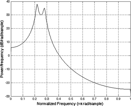

  

  Power spectral density estimate using Yule–Walker method based on 1000 samples

12.2.3 Power Spectrum Estimation Based on AR Model via Burg Method

The Burg method [6] can be used the estimation of the AR model parameters by minimizing the forward and backward errors in the linear predictors. Here we consider the problem of linearly predicting the value of a stationary random process either forward in time (or) backward in time.

Forward Linear Prediction

Here in this case, from the past values of a random process, a future value of the process can be predicted. So, consider one-step forward linear prediction as depicted in Fig. 12.7, for which the predicted value of $y\left( n \right)$ can be written as

Fig. 12.7

One-step forward linear predictor

$$ \overset{\lower0.5em\hbox{$\smash{\scriptscriptstyle\frown}$}}{y} \left( n \right) = - \sum\limits_{k = 1}^{p} {a_{p} (k)y\left( {n - k} \right)} $$

(12.40)

where $\left\{ { - a_{p} (k)} \right\}$ are the prediction coefficients of the predictor of order p.

The forward prediction error is the difference between the value $y\left( n \right)$ and the predicted value $(\overset{\lower0.5em\hbox{$\smash{\scriptscriptstyle\frown}$}}{y} \left( n \right))$ of $y\left( n \right)$ and can be expressed as

$$ \begin{aligned} e_{p}^{f} \left( n \right) & = y\left( n \right) - \overset{\lower0.5em\hbox{$\smash{\scriptscriptstyle\frown}$}}{y} \left( n \right) \\ & = y\left( n \right) + \sum\limits_{k = 1}^{p} {a_{p} (k)} y\left( {n - k} \right). \\ \end{aligned} $$

(12.41)

Backward Linear prediction

In the backward linear prediction, the value $y\left( {n - p} \right)$ of a stationary random process can be predicted from the data sequence $y\left( n \right),y\left( {n - 1} \right), \ldots ,y\left( {n - p + 1} \right)$ of the process. For one-step backward linear prediction of order p, the predicted value of $y\left( {n - p} \right)$ can be written as

$$ \overset{\lower0.5em\hbox{$\smash{\scriptscriptstyle\frown}$}}{y} \left( {n - p} \right) = - \sum\limits_{k = 1}^{p} {a_{p}^{*} (p - k)} y\left( {n + k - p} \right). $$

(12.42)

The difference between $y\left( {n - p} \right)$ and estimate $\dddot y\left( {n - p} \right)$ is the backward prediction error which can be written as denoted as

$$ e_{p}^{b} \left( n \right) = y\left( {n - p} \right) + \sum\limits_{k = 0}^{p - 1} {a_{p}^{*} (k)} y\left( {n + k - p} \right). $$

(12.43)

For lattice filter realization of the predictor, a p-stage lattice filter is described by the following set of order-recursive equation

$$ e_{0}^{f} \left( n \right) = e_{0}^{b} \left( n \right) = x\left( n \right) $$

(12.44a)

$$ e_{m}^{f} \left( n \right) = e_{m - 1}^{f} \left( n \right) + K_{m} e_{m - 1}^{b} \left( {n - 1} \right)\quad m = 1,2, \ldots ,p $$

(12.44b)

$$ e_{m}^{b} = K_{m}^{ * } e_{m - 1}^{f} \left( n \right) + e_{m - 1}^{b} \left( {n - 1} \right)\quad m = 1,2, \ldots ,p $$

(12.44c)

where $K_{m}$ is the mth reflection coefficient in the lattice filter.

A typical stage of a lattice filter is shown in Fig. 12.8.

Fig. 12.8

A typical stage of a lattice filter

From the forward and backward prediction errors, the least squares error for given data $y(n),n = 0,1, \ldots ,N - 1,$ can be expressed as

$$ \varepsilon_{m} = \sum\limits_{n = m}^{N - 1} {\left( {\left| {e_{m}^{f} \left( n \right)} \right|^{2} + \left| {e_{m}^{b} \left( n \right)} \right|^{2} } \right).} $$

(12.45)

Now, the error is to be minimized with respect to predictor coefficients satisfying the following Levinson–Durbin recursion

$$ a_{m} \left( k \right) = a_{m - 1} \left( k \right) + K_{m} a_{m - 1}^{*} \left( {m - k} \right), \quad 1 \le k \le m - 1;1 \le m \le p. $$

(12.46)

where $K_{m} = a_{m} (m)$ is the mth reflection coefficient in the lattice filter of the predictor.

Minimization of $\varepsilon_{m}$ with respect to the reflection coefficient $K_{m}$ yields

$$ \overset{\lower0.5em\hbox{$\smash{\scriptscriptstyle\frown}$}}{K}_{m} = \frac{{ - \sum\nolimits_{n = m}^{N - 1} {e_{m - 1}^{f} \left( n \right)} \left( {e_{m}^{b} \left( n \right)} \right)^{ * } }}{{\frac{1}{2}\overset{\lower0.5em\hbox{$\smash{\scriptscriptstyle\frown}$}}{E}_{m}^{{}} }} $$

(12.47)

where $\overset{\lower0.5em\hbox{$\smash{\scriptscriptstyle\frown}$}}{E}_{m}^{{}}$ is the total squared error which is an estimate of $\overset{\lower0.5em\hbox{$\smash{\scriptscriptstyle\frown}$}}{E}_{m - 1}^{f} + \overset{\lower0.5em\hbox{$\smash{\scriptscriptstyle\frown}$}}{E}_{m - 1}^{b}$, $\overset{\lower0.5em\hbox{$\smash{\scriptscriptstyle\frown}$}}{E}_{m - 1}^{f}$ and $\overset{\lower0.5em\hbox{$\smash{\scriptscriptstyle\frown}$}}{E}_{m - 1}^{b}$ being the least squares estimates of the forward and backward errors given by

$$ \overset{\lower0.5em\hbox{$\smash{\scriptscriptstyle\frown}$}}{E}_{m - 1}^{f} = \sum\limits_{n = m}^{N - 1} {} \left| {e_{m - 1}^{f} \left( n \right)} \right|^{2} $$

(12.48)

$$ \overset{\lower0.5em\hbox{$\smash{\scriptscriptstyle\frown}$}}{E}_{m - 1}^{b} = \sum\limits_{n = m}^{N - 1} {\left| {e_{m - 1}^{b} \left( n \right)} \right|^{2} } . $$

(12.49)

The estimate $\overset{\lower0.5em\hbox{$\smash{\scriptscriptstyle\frown}$}}{E}_{m}^{{}}$ can be computed by using the following recursion

$$ \overset{\lower0.5em\hbox{$\smash{\scriptscriptstyle\frown}$}}{E}_{m}^{{}} = \left( {1 - \left| {\overset{\lower0.5em\hbox{$\smash{\scriptscriptstyle\frown}$}}{K}_{m} } \right|^{2} } \right)\overset{\lower0.5em\hbox{$\smash{\scriptscriptstyle\frown}$}}{E}_{m - 1}^{{}} \left| {e_{m}^{f} \left( {m - 2} \right)} \right|^{2} -^{{}} \left| {e_{m}^{b} \left( {m - 2} \right)} \right|^{2} $$

(12.50)

The Burg method computes the reflection coefficients $\overset{\lower0.5em\hbox{$\smash{\scriptscriptstyle\frown}$}}{K}_{m}$ using Eqs. (12.47) and (12.50), and AR parameters are estimated by using Levinson–Durbin algorithm. Then, the power spectrum can be estimated as

$$ P_{\text{BUR}} \left( f \right) = \frac{{\widehat{E}_{m}^{2} }}{{\left| {1 + \sum\nolimits_{k = 1}^{p} {\widehat{a}_{k} {\text{e}}^{ - j2\pi fk} } } \right|^{2} }}. $$

(12.51)

The following example illustrates the power spectrum estimation using the Burg method.

Example 12.6

Consider the AR process as given in Example 12.5. Evaluate its power spectrum based on 200 samples using the Burg method.

Solution

The MATLAB Program 12.5 can be used by replacing pyulear(y,4,Fs) by pburg(y,4,Fs) to compute power spectrum using the Burg method. Thus, the PSD obtained based on 200 samples using the Burg method is shown in Fig. 12.9.

Fig. 12.9

Power spectral density estimate via Burg method based on 200 samples

The two peaks corresponding to the frequencies $0.22\pi$ and $0.28\pi$ are clearly seen from Fig. 12.9. Using the Burg method based on 200 samples, whereas it is not as shown in Fig. 12.5 using Yule–Walker method for the same number of samples.

The main advantages of the Burg method are high-frequency resolution, stable AR model, and computational efficiency. The drawbacks of the Burg method are spectral line splitting at high SNRs and spurious spikes for high-order models.

12.2.4 Selection of Model Order

Generally, model order is unknown a priori. If the guess for the model order is too low, it will result in highly smoothed spectral estimate and the high-order model increases resolution but low-level spurious peaks will appear in the spectrum. The two methods suggested by Akaike [7, 8] for model order selection are:

• 1. Akaike forward prediction error (FPE) criterion states that

$$ {\mathbf{FPE}}\left( p \right) = \sigma_{{w_{p} }}^{2} \left( {\frac{N + p + 1}{N - p - 1}} \right) $$

(12.52)

should be minimum. Here, N stands for the number of data samples, p is the order of the filter, and $\sigma_{{w_{p} }}^{2}$ is the white noise variance estimate.

• 2. Akaike forward prediction error (FPE) criterion states that

$$ {\mathbf{FPE}}\left( p \right) = N\,\ln (\sigma_{{w_{p} }}^{2} ) + 2p $$

(12.53)

should be minimum.

12.2.5 Power Spectrum Estimation Based on MA Model

By setting p = 0 in Eq. (11.30a) and letting $h(k) = b(k),1 \le k \le q,$ a MA model can be adopted. Then, the model parameters can be related to the autocorrelation sequence as

$$ r_{yy} \left( m \right) = \left\{ {\begin{array}{*{20}c} {\sigma_{\omega }^{2} \sum\nolimits_{k = 0}^{q} {b_{k} b_{k + m} ;} } & {0 \le m \le q} \\ {0;} & {m > q} \\ {r_{yy}^{*} \left( { - m} \right);} & {m < 0} \\ \end{array} } \right.. $$

(12.54)

Then, the power spectrum estimate based on MA model is

$$ P_{{{\mathbf{MA}}}} \left( f \right) = \sum\limits_{m = - q}^{q} {r_{yy} \left( m \right)} \;{\text{e}}^{ - j2\pi fm} . $$

(12.55)

Equation (12.55) can be written in terms of MA model parameter estimates $\left( {\overset{\lower0.5em\hbox{$\smash{\scriptscriptstyle\frown}$}}{b}_{k} } \right)$, and the white noise variance estimate $(\overset{\lower0.5em\hbox{$\smash{\scriptscriptstyle\frown}$}}{\sigma }_{{w_{{}} }}^{2} )$ can be written as

$$ P_{MA} \left( f \right) = \overset{\lower0.5em\hbox{$\smash{\scriptscriptstyle\frown}$}}{\sigma }_{{w_{{}} }}^{2} \left| {1 + \sum\limits_{k = 1}^{q} {\overset{\lower0.5em\hbox{$\smash{\scriptscriptstyle\frown}$}}{b}_{k} \;{\text{e}}^{ - j2\pi fk} } } \right|^{2} . $$

(12.56)

12.2.6 Power Spectrum Estimation Based on ARMA Model

ARMA model is used to estimate the spectrum with less parameters. This model is mostly used when data is corrupted by noise.

The AR parameters are estimated first, independent of the MA parameters, by using the Yule–Walker method or the Burg method. The MA parameters are estimated assuming that the AR parameters are known.

Then, the ARMA power spectral estimate is

$$ P_{\text{ARMA}} \left( f \right) = \overset{\lower0.5em\hbox{$\smash{\scriptscriptstyle\frown}$}}{\sigma }_{{w_{{}} }}^{2} \left| {\frac{{1 + \sum\nolimits_{k = 1}^{q} {\overset{\lower0.5em\hbox{$\smash{\scriptscriptstyle\frown}$}}{b}_{k} {\text{e}}^{ - j2\pi fk} } }}{{1 + \sum\nolimits_{k = 1}^{p} {\overset{\lower0.5em\hbox{$\smash{\scriptscriptstyle\frown}$}}{a}_{k} {\text{e}}^{ - j2\pi fk} } }}} \right|^{2} . $$

(12.57)

12.3 Subspace Methods for Power Spectrum Estimation

The subspace methods do not assume any parametric model for power spectrum estimation. They are based solely on the estimate of the autocorrelation sequence of the random process from the observed data. In this section, we briefly discuss three subspace methods, namely, Pisarenko harmonic decomposition, MUSIC, and eigenvector method.

12.3.1 Pisarenko Harmonic Decomposition Method

Consider a process y consisting of m sinusoids with additive white noise. The autocorrelation values of the process y can be written in matrix form as

$$ \left[ {\begin{array}{*{20}c} {r_{{yy}} (1)} \\ {r_{{yy}} (2)} \\ \vdots \\ {r_{{yy}} (m)} \\ \end{array} } \right] = \left[ {\begin{array}{*{20}c} {{\text{e}}^{{j2\pi f_{1} }} } & {{\text{e}}^{{j2\pi f_{2} }} } & {{\text{e}}^{{j2\pi f_{3} }} } & \ldots & {{\text{e}}^{{j2\pi f_{m} }} } \\ {{\text{e}}^{{j4\pi f_{1} }} } & {{\text{e}}^{{j4\pi f_{2} }} } & {{\text{e}}^{{j4\pi f_{3} }} } & \ldots & {{\text{e}}^{{j4\pi f_{m} }} } \\ \vdots & \vdots & \vdots & \ldots & \vdots \\ {{\text{e}}^{{j2\pi mf_{1} }} } & {{\text{e}}^{{j2\pi mf_{2} }} } & {{\text{e}}^{{j2\pi mf_{3} }} } & \ldots & {{\text{e}}^{{j2\pi mf_{m} }} } \\ \end{array} } \right]\left[ {\begin{array}{*{20}l} {P_{1} } \hfill \\ {P_{2} } \hfill \\ \vdots \hfill \\ {P_{m} } \hfill \\ \end{array} } \right] $$

(12.58)

where $P_{i}$ is the average power in the ith sinusoid.

If the frequencies $f_{i} ,^{{}} 1 \le i \le m,$ are known, then from the known autocorrelation values $r_{yy} (1)$ to $r_{yy} (m),$ the sinusoidal powers can be determined from the above equation.

The stepwise procedure for the Pisarenko harmonic decomposition method is as follows.

• Step 1: Estimate the autocorrelation vector from the observed data.

• Step 2: Find the minimum eigenvalue and the corresponding eigenvector $(v_{m + 1} )$

• Step 3 : Find the roots of the following polynomial

$$ \sum\limits_{k = 0}^{M} {v_{m + 1} (k + 1)} z^{ - k} $$

(12.59)

where $v_{m + 1}$ is the eigenvector. The roots lie on the unit circle at angles $2\pi f_{i}^{{}}$ for $1 \le i \le M,$M is dimension of eigenvector,

Step 4 : Solve Eq. (12.58.) for sinusoidal powers $(P_{i} )$.

12.3.2 Multiple Signal Classification (MUSIC) Method

The MUSIC estimates the power spectrum from a signal or a correlation matrix using Schmidt’s eigen space analysis method [9]. The method estimates the signal’s frequency content by performing eigen space analysis of the signal’s correlation matrix. In particular, this method is applicable to signals that are the sum of sinusoids with additive white Gaussian noise and more, in general, to narrowband signals. To develop this, first let us consider the ‘weighted’ spectral estimate

$$ P\left( f \right) = S^{H} (f)\left( {\sum\limits_{k = m + 1}^{M} {c_{k} V_{k}^{{}} V_{k}^{H} } } \right)S(f) = \sum\limits_{k = m + 1}^{M} {c_{k} } \left| {S^{H} \left( f \right)V_{k} } \right|^{2} $$

(12.60)

where m is the dimension of the signal subspace, $V_{k}$, $k = m + 1, \ldots ,M$ are the eigen vectors in the noise subspace, $c_{k}$ are a set of positive weights, and

$$ S\left( f \right) = \left[ {1,{\text{e}}^{j2\pi f} ,{\text{e}}^{j4\pi f} , \ldots ,{\text{e}}^{j2\pi (m - 1)f} } \right]\,\text{is\,complex\,sinusoidal\,vector}. $$

It may be noted that at $f = f_{i}$, $S\left( {f_{i} } \right) = S_{i} ,$ such that at any one of the p sinusoidal frequency components of the signal we have,

$$ P\left( {f_{i} } \right) = 0\quad i = 1,2, \ldots ,m. $$

(12.61)

This indicates that

$$ \frac{1}{P\left( f \right)} = \frac{1}{{\sum\nolimits_{k = m + 1}^{M} {c_{k} \left| {S^{H} \left( f \right)V_{k} } \right|^{2} } }} $$

(12.62)

is infinite at $f = f_{i} .$ But, in practice due to the estimation errors, $\frac{1}{P\left( f \right)}$ is finite with very sharp peaks at all sinusoidal frequencies providing a way for estimating the sinusoidal frequencies.

Choosing $c_{k} = 1$ for all k, the MUSIC frequency estimator [10] is written as

$$ P_{{{\mathbf{MUSIC}}}} \left( f \right) = \frac{1}{{\sum\nolimits_{k = m + 1}^{M} {\left| {S^{H} \left( f \right)V_{k} } \right|^{2} } }} $$

(12.63)

The peaks of $P_{{{\mathbf{MUSIC}}}} \left( f \right)$ are the estimates of the sinusoidal frequencies, and the powers of the sinusoids can be estimated by solving Eq. (12.58). The following example illustrates the estimation of power spectrum using the MUSIC method.

Example 12.7

Consider a random signal generated by the following equation

$$ x(n) = \sin \left( {\frac{{2\pi f_{1} n}}{{F_{\text{s}} }}} \right) + 2\sin \left( {\frac{{2\pi f_{2} n}}{{F_{\text{s}} }}} \right) + 0.1w(n) $$

where the frequencies f ₁ and f ₂ are 220 and 332 Hz, respectively, the sampling frequency F_s is 2048 Hz and $w(n)$ is a zero mean, unit variance, white noise process. Estimate power spectrum of the sequence $\left\{ {x(n),0 \le n \le 1023} \right\}.$

Solution

The MATLAB function pmusic(X,m,‘whole’) gives the power spectrum of a discrete-time signal X using the MUSIC method, m being the number of complex sinusoids in the signal X. If X is an autocorrelation data matrix of discrete-time signal x, the function corrmtx can be used to generate data matrices. The signal vector x consists of two real sinusoidal components. In this case, the dimension of the signal subspace is 4 because each real sinusoid is the sum of two complex exponentials.

The following MATLAB Program 12.6 is used to obtain the power spectrum using the MUSIC method.

Program 12.6

• Power spectrum estimation using the MUSIC method

• clear;clc;

• randn('state',0);

• N = 1024;%total number of samples

• k = 0 : N-1;

• f1 = 280;

• f2 = 332;

• F_T = 2048;%sampling frequency in Hz

• T = 1/F_T;

• x = sin(2*pi*f1*k*T) + 2*sin(2*pi*f2*k*T)+0.1*randn(size(k));%input vector of length N

• X = corrmtx(x,12);%estimates (N+12) by (12+1) rectangular autocorrelation matrix

• pmusic(X,4,'whole'); %estimates power spectrum of x containing two sinusoids

• The power spectrum obtained from the above program is shown in Fig. 12.10.

  Fig. 12.10

  

  Power spectral density estimate using MUSIC method

12.3.3 Eigenvector Method

The eigenvector method is a weighted version of the MUSIC method. Selecting $c_{k} = \frac{1}{{\lambda_{k} }}$ in Eq. (12.62) for all k, the eigenvector method produces a frequency estimator given by Johnson [11].

$$ P_{\text{eig}} \left( f \right) = \frac{1}{{\left( {\mathop \sum \nolimits_{k = m + 1}^{M} \left( {\frac{1}{{\lambda_{k} }}} \right)\left| {V_{k}^{H} S\left( f \right)} \right|^{2} } \right)}} $$

(12.64)

where M is the dimension of the eigenvectors and $V_{k}$ is the kth eigenvector of the autocorrelation matrix of the observed data sequence. The integer m is the dimension of the signal subspace, so the eigenvectors $V_{k}$ used in the sum correspond to the smallest eigenvalues $\lambda_{k}^{{}}$ of the autocorrelation matrix. The eigenvectors used in the PSD estimate span the noise subspace. The power spectrum estimation using the eigenvector method is illustrated through the following example.

Example 12.8

Consider the random signal generated in the Example 12.7 and estimate its power spectrum using the eigenvector method.

Solution

The MATLAB function peig(X,m,‘whole’) estimates the power spectrum of a discrete-time signal X, m being the number of complex sinusoids in the signal X. If X is an autocorrelation data matrix of discrete-time signal x, the function corrmtx can be used to generate data matrices. The signal vector x consists two real sinusoidal components. In this case, the dimension of the signal subspace is 4 because each real sinusoid is the sum of two complex exponentials.

The following MATLAB Program 12.7 is used to obtain the power spectrum using the eigenvector method.

• Program 12.7

• Power spectrum estimation using the eigenvector method

• clear;clc;

• randn('state',0);

• N = 1024;%total number of samples

• k = 0 : N-1;

• f1 = 280;

• f2 = 332;

• F_T = 2048;%sampling frequency in Hz

• T = 1/F_T;

• x = sin(2*pi*f1*k*T)+2*sin(2*pi*f2*k*T)+0.1*randn(size(k));%input vector of length N

• X = corrmtx(x,12);%estimates (N+12) by (12+1) rectangular autocorrelation matrix

• peig(X,4,'whole');%estimates power spectrum of x containing two sinusoids

• The power spectrum produced from the above program is shown in Fig. 12.11.

  Fig. 12.11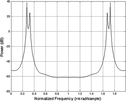

  

  Power spectral density estimate using eigenvector method

12.4 Spectral Analysis of Non-stationary Signals

A signal with time-varying parameters, for example, a speech signal, is called a non-stationary signal. The spectrogram which shows how the spectral density of a signal varies with time is a basic tool for spectral analysis of non-stationary signals. Spectrograms are usually generated using the short-time Fourier transform (STFT) using digitally sampled data. To compute the STFT, a sliding window which usually is allowed to overlap in time is used to divide the signal into several blocks of data. Then, an N-point FFT is applied to each block of data to obtain the frequency contents of each block.

The window length affects the time resolution and the frequency resolution of the STFT. A narrow window results in a fine time resolution but a coarse frequency resolution, whereas a wide window results in a fine frequency resolution but a coarse time resolution. A narrow window is to be used to provide wideband spectrogram for signals having widely varying spectral parameters. A wide window is preferred to have narrowband spectrogram. The following example illustrates the computation of the spectrogram of a speech signal.

Example 12.9

Consider a speech signal ‘To take good care of yourself’ from the sound file ‘goodcare.wav’ (available in the CD accompanying the book). Compute the spectrogram of the speech signal using Hamming window of lengths 256 samples and 512 samples with an overlap of 50 samples.

Solution

The STFT of a non-stationary signal x can be computed by using the MATLAB file specgram(x,wl,Fs, window,noverlap)

where wl stands for window length, and noverlap is the number of overlap samples.

• Program12.8

• Spectrogram of a speech signal

• [x,F_T] = wavread('goodcare.wav');

• i = 1:length(x)

• figure(1),plot(x)

• xlabel(‘Time index i’);ylabel('Amplitude');

• figure(2), specgram(x,256, F_T,hamming(256),50)

• The speech signal 'To take god care of yourself' is shown in Fig. 12.12.

  Fig. 12.12

  

  A speech signal

  Fig. 12.13

  

  a Spectrogram with window length 256, overlap = 50 and b spectrogram with window length 512, overlap = 50

• The spectrograms of the speech signal for window lengths of 256 and 512 samples are shown in Fig. 12.13a, b respectively.

• From the above spectrograms, the trade-off between frequency resolution and time resolution is evident.

12.4.1 MATLAB Exercises

• 1. Consider a random signal of length 1024 composed of two sinusoidal components of frequencies 180 and 320 Hz with sampling frequency of $F_{T}$ = 2048 Hz corrupted with zero mean, unit variance, white noise process. Evaluate its power spectrum using Bartlett’s method with subsequence lengths of each 256 samples.

• 2. Consider the following signal of length N = 1024 with sampling frequency of F_s = 2048 Hz corrupted with zero mean, unit variance, white noise process.

$$ x\left( i \right) = \sin \left( {\frac{800\pi i}{{F_{T} }}} \right)\cos \left( {\frac{800\pi i}{{F_{T} }}} \right) + w\left( i \right),\quad 0 \le i < N $$

where $w(i)$ is zero mean Gaussian white noise.

Evaluate its power spectrum using Welch’s method with subsequence lengths of each 256 samples using Blackman window for overlaps of 64 and 128 samples, respectively.

• 3. Consider the following signal of length N = 1024 with sampling frequency of F_s = 2048 Hz corrupted with zero mean, unit variance, white noise process.

$$ x\left( i \right) = \sin^{2} \left( {\frac{400\pi i}{{F_{T} }}} \right)\cos^{2} \left( {\frac{200\pi i}{{F_{T} }}} \right) + w\left( i \right), \quad 0 \le i < N $$

where $w(i)$ is zero mean unit variance, white noise process.

Evaluate its power spectrum using Blackman–Tukey method with window length of 256 samples.

• 4. Consider a fourth-order AR process characterized by

$$ y(n) + a_{1} y(n - 1) + a_{2} y(n - 2) + a_{3} y(n - 3) + a_{4} y(n - 4) = w(n) $$

where $w(n)$ is a zero mean, unit variance, white noise process. The parameters $\left\{ {a_{1} ,a_{2} ,a_{3} ,a_{4} } \right\}$ are chosen such that the prediction error filter

$$ A(z) = 1 + a_{1} z^{ - 1} + a_{2} z^{ - 2} + a_{3} z^{ - 3} + a_{4} z^{ - 4} $$

has zeros at the locations.

$$ 0.98{\text{e}}^{ \pm j0.15\pi } \;{\text{and}}\;0.98{\text{e}}^{ \pm j0.35\pi } $$

Estimate the power spectrum of the AR process using the Yule–Walker method and Burg method based on 200 samples. Comment on the results.

• 5. Consider the following signal of length N = 1024 with sampling frequency of F_s = 2048 Hz corrupted with zero mean, unit variance, white noise process.

$$ x\left( n \right) = \sum\limits_{i = 1}^{3} {{\text{e}}^{{j2\pi f_{i} n}} } + w\left( n \right), \quad 0 \le n < N $$

where $w(i)$ is zero mean unit variance, white noise process, and the frequencies are Hz $f_{1} = 256\,{\text{Hz}},f_{2} = 338\,{\text{Hz}},$ and $f_{3} = 338\,{\text{Hz}}.$

Evaluate its power spectrum using the MUSIC method and the eigenvector method. Comment on the results.

• 6. Consider a speech signal from the sound file ‘speech.wav’ (available in the CD accompanying the book) and compute its spectrogram for different window lengths with and without overlap. Comment on the results.

References

A. Schuster, On the investigation of hidden periodicities with application to a supposed 26 day period of meteorological phenomena. Terr. Magn. Atmos. Electr. 3, 13–41 (1898)
M.S. Bartlett, Smoothing periodograms from time series with continuous spectra. Nature 161, 686–687 (1948)
P.D. Welch, The use of fast Fourier transform for the estimation of power spectra: A method based on time averaging over short, modified periodograms. IEEE Trans. Audio Electroacoust. 15, 70–83 (1967)
R.B. Blackman, J.W. Tukey, The Measurement of Power Spectra from the Point of View of Communication Engineering (Dover Publications, USA, 1958)
J.G. Proakis, D.G. Manolakis, Digital Signal Processing Principles, Algorithms and Applications (Printice-Hall, India, 2004)
J.P. Burg, A new Analysis technique for time series data. Paper presented at the NATO Advanced Study Institute on Signal Processing, Enschede, 1968
H. Akaike, Power spectrum estimation through autoregressive model fitting. Ann. Inst. Stat. Math. 21, 407–420 (1969)
H. Akaike, A new look at the statistical model identification. IEEE Trans. Autom. Control 19(6), 716–723 (1974)
S.L. Marple, in Digital Spectral Analysis. (Prentice-Hall, Englewood Cliffs, NJ, 1987), pp. 373–378, 686–687
R.O. Schmidt, Multiple emitter location and signal parameter estimation. IEEE Trans. Antennas Propag. AP-34, 276–280 (1986)
D.H. Johnson, The application of spectral estimation methods to bearing estimation problems. Proc. IEEE 70(9), 126–139 (1982)
Author information
Authors and Affiliations
Corresponding author
Rights and permissions
Copyright information
© 2018 Springer Nature Singapore Pte Ltd.
About this chapter
Cite this chapter
Rao, K., Swamy, M. (2018). Spectral Analysis of Signals. In: Digital Signal Processing. Springer, Singapore. https://doi.org/10.1007/978-981-10-8081-4_12
Download citation
DOI: https://doi.org/10.1007/978-981-10-8081-4_12
Published:
Publisher Name: Springer, Singapore
Print ISBN: 978-981-10-8080-7
Online ISBN: 978-981-10-8081-4
eBook Packages: Mathematics and StatisticsMathematics and Statistics (R0)