Simple Programs

Abstract

Normally a computational task is spelt out in pseudo code form or as a flowchart. Forming the program code with this as guide is good practice. The task can be simple and direct or conditional. The latter is often realized using keywords like while or if. They are explained through clear and focused examples. The idea of iterative routines, their convergence to a solution of desired accuracy using judgment based on metrics to stop iteration—all these go with these. A few widely used approaches to iterative solutions are explained here. The variety of exercises given, help in understanding the types of tasks as well as possible iterative procedures.

These keywords were added by machine and not by the authors. This process is experimental and the keywords may be updated as the learning algorithm improves.

As was seen in the last two chapters basic algebraic operations are carried out in Python as with a simple calculator. More involved operations call for preparation of programs and working with them. The program structure in Python has to conform to specific syntactic rules. These are to be religiously followed to ensure that Python interprets the program for subsequent execution (van Rossum and Drake 2014).

3.1 Basic Program Structure

Even the simplest of programs calls for a sequence of computations/activities to be executed with its associated constraints (Guttag 2013). Let us take such a simple program by way of illustration.

Example 3.1

Compute the sum of n _r natural numbers.

The steps [1]–[5] in the sequence in Fig. 3.1 achieve this for n _r = 12; the result is output—[6] and the related output in the following line. Any other (positive) integral value can be assigned to n _r and the corresponding sum computed in the same manner.

Fig. 3.1

Python Interpreter sequence for Examples 3.1 and 3.2

Figure 3.2 aids the understanding of the program and its working. ‘ while ’ is a keyword. ‘ while i:’ tests the value of i; as long as it is True —that is it is non-zero—the group of statements following is executed. The colon ‘:’ following i signifies this. This set of statements forming the group is to be indented with respect to the beginning of the line (incidentally in Python such a group is often referred to as a ‘suite’). The indentation can be achieved through tabs or spaces. But all the statements within the group should have the same indentation—done consistently with tabs or spaces (preferably spaces). One line left free after the group [4] and [5] here—signifies the end of the group. In the specific program here if i (equal to n _r) at the start is non-zero, it is added to the sum [4] and decremented [5]. The sequence continues until i becomes zero; i.e., n _r (12), n _r − 1 (11), n _r − 2 (10), … 2, and 1 are all successively added to the sum. Once the loop operation is over the program proceeds to the following line [6] and continues execution. Here the values of n _r and sums are printed out. The simplicity of the loop structure is striking. There is no need to put parentheses around the condition to be tested, no need to identify the group by enclosing it within curly brackets and so on. The group may have as many executable statements as desired. The whole condition is checked after every execution of the group sequence.

Fig. 3.2

Structure of the program for the sequence [1]–[6] in Fig. 3.1 (Example 3.1)

Example 3.2

Identify all the numbers in the interval {100 to 200} which are divisible by 13 and output them.

The 6-line program from [7]–[11] achieves this; it is a bit more involved compared to the previous one. The program accepts three integers—l1 (lower limit), l2 (upper limit), and a specified number n—and prints out all the numbers between l1 and l2 which are divisible by n. j—a dummy/running variable—is assigned the value of the lower limit to start with. Two successive checks are done on j. First check whether j < l2; if so enter the loop/continue within the loop execution. Within the loop 1 check whether j is divisible by n. If so enter loop 2 and execute it. Else do not enter loop 2/keep away from it. Loop 2 here demands a single action—print the value of the number and proceed to the next line. Once you exit loop 2, you are back in loop 1. Increment the value of j [11]. This forms the last line of the program within loop 1. In the specific case here all numbers in the interval—100–200—that are divisible by 13 are printed out in the same sequence as they are encountered.

The program brings out a number of additional aspects of Python.

• Loop 2 is within loop 1. All statements within loop 2 form a sub-group. (Incidentally loop 2 has only a single statement here.) They appear with the same indentation within loop 1 (see Fig. 3.3).

  Fig. 3.3

  

  Structure of the program for the sequence [7]–[11] in Fig. 3.1 (Example 3.2)

• ‘ if ’ is a keyword. It is used to check a condition and execute a loop if the condition is satisfied.

• The operator ‘==’ checks whether the values of quantities on either side are identical. Specifically here if j%n is zero, j%n == 0 is true (or 1); if it is non-zero, it is false (or 0).

Incidentally if a loop has only a single statement in it, the same can follow the condition on the same line. The Python Interpreter sequence is as in Fig. 3.4.

Fig. 3.4

The sequence in Fig. 3.3 with its loop 2 being in a single line

Any normal/useful program will require a sequence of activities (representing the corresponding executable statements) to be carried out. The sequence will be linked through specific conditional decisions (as in the two small illustrations above). It is necessary to conceive of the overall computation, fully understand the same, represent it in a clear logical sequence and then do the program coding. Such a structured representation is conveniently done in ‘pseudo-code ’ form. It is good programming practice to represent the program in pseudo-code form and then proceed with the coding proper. The pseudo code for a program with one conditional loop within is shown in Fig. 3.5a; Example 3.1 can be seen to be of this type. The pseudo-code in Fig. 3.5b has two conditional loops—loop 2 being executed within loop 1; Example 3.2 can be seen to be of this type. The following are noteworthy here:

Fig. 3.5

a Pseudo codes for the sequence in Fig. 3.1: a First example and b Second example

• Any sequence of executions which does not involve conditional checks is represented by one/a few statements. The suite of these statements together constitutes one logical block to be executed. ‘begin’ and ‘end’ signify the beginning and the end of the block/suite.

• Every logical block is entered after a conditional check. To clarify this, the logical block is identified through a definite indent on the left of the parent block.

• For successive logical checks followed by corresponding logical blocks similar indentations are used.

In general the pseudo code of a program may involve a number of conditional loops in a sequence; some of these loops may have single or multiple loops within in cascaded/sequential forms. A number of such pseudo code structures appear with the examples to follow here as well as in subsequent chapters.

The pseudo code representation of the program enables the programmer to conceive of the program in its totality, identify the conditions and activities at the highest level and represent it in a compact form. Subsequently each of the activities identified can be looked into separately and split into separate connected conditional blocks (See Fig. 3.6). The process can be continued as much as necessary; finally each block in the representation can be coded separately. All such coded blocks can be combined conforming to the representations at different stages and finally the overall program can be realized. This is the ‘top down’ approach used for the program. The approach has many advantages:

Fig. 3.6

‘Top down’ approach to pseudo code representation

• Visualization of the program in the proper perspective—in terms of major blocks and their connections/links at the top level.

• Identification of the activities at each block, their connections, and sequences.

• Clarity in visualization and program realization.

• Easiness in testing and debugging: each of the identified smallest blocks can be programmed, tested, and debugged separately and blocks combined in a step by step manner.

• With large programs different segments can be developed individually, and (if necessary) separately by different groups. All segments can be knitted together with the least interface problems.

3.2 Flow Chart

Flow chart is an alternate form of representation of computer programs. Each identified activity in a program is represented as a block and the program conceived as a group of blocks connected through lines and arrows representing program flow. Figure 3.7 shows a simple flow chart. Start and stop—the beginning and end of the program are represented with respective circles. Inputs and outputs are identified through double-line oblong enclosures shown. Executable groups of statements are represented by rectangular blocks. The flow chart in Fig. 3.7 has four such executable block segments. The diamond (or a rhombus in its place) is a decision block. It represents a condition to be tested and the resulting branching. There may be two or more branches on the output side of a conditional block. A decision/branching is a key element in a flow chart. It steers the program conforming to the logical process desired. The blocks are connected through lines with arrows showing directions of program flow. In general a program represented by a flow chart progresses downwards. The flowcharts for the two examples considered earlier are shown in Fig. 3.8.

Fig. 3.7

A typical flowchart structure

Fig. 3.8

Flowcharts for a Example 3.1 and b Example 3.2

Flow charts of programs encountered in practice can be much more involved—involving a number of decision blocks, and executable blocks. Well thought out programs can be represented as well organized flow charts. In turn it helps the coding and execution considerably.

The choice of a pseudo code or a flowchart for a program is purely a subjective one. When embarking on preparing a program for a task, the need to clearly conceive the program task, and represent it in the form of a flow chart or a pseudo code with full logic flow and interlinking fully clarified, need hardly be stressed.

3.3 Conditional Operations

A select set of keywords helps to test conditions and steer program. Their usage is brought out through a set of examples here.

Example 3.3

Output the sum of squares of the first eight odd integers.

The segment [1]–[4] in the python Interpreter sequence in Fig. 3.9 computes the desired sum—sum of squares of the eight odd integers starting with 1—and outputs the same (=680). Here n is a counter—initialized to 8 and counting is done downwards until n is zero. The loop starting with ‘ while’ is executed as long as n ≠ 0; ‘ while’ is a keyword here. n = 0 is interpreted as ‘ False ’ and causes termination of the loop execution. The flow chart for the program is shown in Fig. 3.10; it can be seen to be similar to the flowchart in Fig. 3.8a as far as functional blocks and program flow are concerned. In the print statement [3] the function repr (sm) converts sm to a printable string. It is concatenated with the string ‘the required sum is’ and the combination output in a convenient form. [4] is possibly a simpler print version. The print function outputs the string and sn directly.

Fig. 3.9

Python Interpreter sequence for Examples 3.3 and 3.4

Fig. 3.10

Flowchart for Example 3.3 (Interpreter sequence [1]–[4] in Fig. 3.9)

‘ True ’ and ‘ False ’ are keywords; they are the Boolean values equivalent to 1 and 0 respectively. Their use is illustrated through the following example.

Example 3.4

Identify the first seven positive integers and output the sum of their cubes.

The routine [5]–[8] in the sequence in Fig. 3.9 obtains the desired sum and outputs the same. As in the previous program n counts down from 8. a is assigned the ‘ True ’ value initially. The loop execution continues as long as the status of a remains True . It is changed to False in the loop when n becomes zero [7]. [7] illustrates the use of keyword ‘ if ’. Like ‘ while ’, the ‘ if ’ statement checks for a condition; on the condition being satisfied, the statement (group of statements) following is (are) executed. The condition being tested is whether n == 0. If the condition is true—that is n is zero—the statement specified is executed (a is assigned the value False ). In turn execution terminates here. The sum (444,528) is output following line [8]. The flowchart is similar to that in Fig. 3.10 and is not shown separately.

The Python Interpreter sequence in Fig. 3.11 illustrates use of some additional features basic to Python programs, again through examples.

Fig. 3.11

Python Interpreter sequence for Examples 3.5, 3.6, and 3.7

Example 3.5

What is the total number of positive integers below 200 which are divisible by 11?

The routine [1]–[4] in Fig. 3.11 obtains this number. There are altogether 18 of these numbers as can be seen from the line following [4]. The program is also an illustration for the use of keyword ‘ is ’.

Here the condition ‘a’ being true is being tested in [2] with the use of ‘ is ’. The block of three executable statements up to [3] is executed as long as a is True . As soon as a =  False the loop execution stops. The operation ‘ is not ’ can be used similarly. ‘a is not b’ has value ‘ True ’ as long as a and b are not identical.

Example 3.6

Identify all the numbers between 100 and 1000 which are divisible by 11 and 13 and output them.

The program sequence [5]–[8] in Fig. 3.11 identifies and outputs these numbers. The condition that the number represented by b is divisible by 11 (b%11 == 0) as well as by 13 (b%13 == 0) is tested using the single condition in [7]. It uses the logical operator ‘ and’ —a keyword; p and q is True only if p is True and simultaneously q is also True . The logical operator ‘or’ can be used in a similar manner. p or q is True if either p is True or q is True .

Example 3.7

Identify the smallest number greater than 10000 which is a power of 29.

The routine follows from [9] in Fig. 3.11. Starting with 29 we take its successive powers. The process is continued without break until the number crosses the value 10000. Once this value is crossed execution breaks out of the loop as specified by [11]. ‘break’—a keyword—exits from the current loop on the specified condition being true. ‘while True’ is always true: hence in the absence of the conditional break statement within, the loop execution will continue ad infinitum. Incidentally the desired number here is 24,389(=29³).

Example 3.8

Obtain the sum of the cubes of all positive integers in the range [0, 10] which have 3 as a factor.

The segment [1]–[4] in the Python Interpreter sequence in Fig. 3.12 is the relevant program. This simple example also illustrates the use of the ‘ range ()’ function.

Fig. 3.12

Python Interpreter sequence for Examples 3.8 and 3.9

The scope of the range function is clarified in Fig. 3.13. range () specifies a sequence of integers—often used to carry out an iteration as done here. The first integer signifies the start for the range and the second one its termination. The first can be absent in which case the default value is taken as zero. The third stands for the interval for the range; if absent the default interval value is taken as unity. All the three integers can be positive or negative. The range specification should be realizable.

Fig. 3.13

Structure and scope of range () in Python: Note that a, b, and c should be integers or functions which return an integer

• range (5), range (0, 5), range (0, 5, 1) all these specify the range {0, 1, 2, 3, 4}.

• range (−2, 3, 1) and range (−2, 3) specify the same range {−2, −1, 0, 1, 2}

• range (10, −5, −2) implies the range {10, 8, 6, 4, 2, 0, −2, −4}.

• range (2, 4, −1) is erroneous.

In the context here the suite of executable statements—in fact the single one in [2]: sm += i³ is executed over a specified range—namely 0–10 with an interval of 3. The routine outputs the sum 3³ + 6³ + 9³ as can be seen from [3]. [4] also achieves the same output. Both are shown here to bring out the fact that a string can be specified through ‘… ’ or “…’’.

Example 3.9

In the range [2, 10] identify the integers as ‘odd’ or ‘even’ and output accordingly.

The sequence [5]–[8] in Fig. 3.12 executes the desired task. It also illustrates the use of the keyword ‘ continue’ . The outer loop is executed for all m in the range 2–10. If (n%2 == 0)—that is n is an even number—the value is output as an ‘even number’. Then the routine continues with the loop—ignoring the sequence following. This is implied by ‘ continue’ . Of course if n is odd, (n%2 == 0) is not satisfied and the loop execution continues with the rest of the executable lines. Here the number concerned is output as an ‘odd number’. If the ‘ continue’ is replaced by ‘ break’ the loop will terminate after the first execution following satisfaction of condition (n% == 0)—after the first even number (=2) is output. The program has been repeated as a sequence following [9] with ‘ continue’ being absent. Here the even numbers are output with an ‘even number’ tag. Apart from this they are also output with tag ‘number’ since line [8] is also executed here. The program is included here to clarify the role of the keyword—‘ continue’ .

3.4 Iterative Routines

Consider the quadratic equation

$$ px^{ 2} + qx + r = 0 $$

where p, q, and r are constants. The solutions can be directly obtained using the formula

$$ x = \frac{{ - q \pm \sqrt {q^{2} - 4pr} }}{2p} $$

If p = 1, q = −3, and r = 2, we get 1 and 2 as the possible solutions. There are a number of situations where a solution cannot be obtained directly in this manner. A widely adopted procedure is to select an appropriate iterative method of solving such equations (Kreyszig 2006). Let us illustrate this through an example.

Example 3.10

Find the cube root of 10.

It is implicitly assumed here that we do not have access to log tables or calculator based procedures which yield the cubic root directly. We fall back on a ‘trial and error’ approach—a binary search. The procedure involves the following steps:

• 1. Let a = 10—a is assigned the value of the number whose cube root we seek.

• 2. Starting with b = 1, get b3 as b ³.

• 3. Increment b and get its cube. Do this successively until b ³ exceeds a.

• 4. Now we know that the cube root of a lies between the last value of b and that of b − 1. Let b 1 = b − 1 and b2 = b. This completes the first part of the iteration.

• 5. Compute bm—the mean of b1 and b2 as bm = (b1 + b2)/2.

• 6. Obtain bm ³. If bm ³ > a, we know that the cube root of a lies between b1 and bm. Assign bm to b2 as b2 = bm. Proceed to step 8.

• 7. If bm ³ ≤ a in step 6, we know that the cube root of a lies between bm and b2. Assign bm to b1 as b1 = bm.

• 8. If bm and b1 (or bm and b2) are sufficiently close, we take bm as the cube root value with the desired level of accuracy; else we go back to step 5.

• 9. The iterative procedure outlined above is depicted in flowchart form in Fig. 3.14. The Python code for the example is in Fig. 3.15.—[1]–[6]. The result is in [7]. We have introduced a counter—‘n’—in the routine to keep track of the number of iterations gone through. If n exceeds a preset limit we terminate the program. Here the limit has been set as 20. When execution is completed we get the desired cube root of a as 2.1552734375; the solution is after 10 iterative cycles.

  Fig. 3.14

  

  Flowchart for Example 3.10

  Fig. 3.15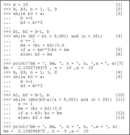

  

  Python iterative sequence for Example 3.10

The routine also illustrates the use of keyword—‘ else ’. else is always used in combination with if to steer a routine through one or the other alternative code groups. The iteration process—reduction in the search range of solution in successive iteration cycles gone through is depicted in Fig. 3.16. The following are noteworthy here:

Fig. 3.16

Narrowing of the search range in successive iterations for Example 3.10

• The approach followed is of a ‘divide and conquer’ type; with each successive step the search range is halved. In turn the % error or indecision in the value of the cube root obtained is also halved.

• Since 2⁻¹⁰ = 1/1024, the condition b1 – b2 ≤ 0.001 (=1/1000) is achieved in 10 successive iterations. Hence n = 10 when the iteration stops.

• If ε denotes the accuracy specified (ε = 0.001 here), as ε reduces the number of iterative cycles required to achieve the specified accuracy increases. In fact the number of iterative cycles required is $\left\lceil { - { \log }_{2}\upvarepsilon} \right\rceil$.

• Beyond a limit the cumulative effect of truncation errors will dominate, preventing further improvement in accuracy (error propagation is not of direct interest to us here).

• 2.1552734375³ – 10 = 0.01168391. The fractional error in the cube value is 0.001168391 = 0.117%.

• The program is run with the termination condition altered to that in [11] in Fig. 3.15. The accuracy for termination is specified in terms of the cube value (in contrast to the last case where it was in terms of the cube root value). The program stops after nine iterations. The cube root value obtained is 2.154296875. Correspondingly the fractional error is |(2.154296875³ – 10)|/10 = 0.0001919.

As mentioned earlier the successive bifurcation procedure outlined here can be used to seek solution for a variety of equations. More often we seek solutions for x such that f(x) = 0 where f(x) is a specified function of x. For the above case f(x) = 10 – x ³. In all these cases we should have a clear prior idea of the possible range of solutions and the number of solutions in the range. This is to prevent a ‘wild-goose-chase’ situation.

The sequence in Fig. 3.17 is a slightly altered approach to the problem in Example 3.10. Here the search interval in every iterative cycle is reduced to 1/3rd of the preceding one—[1] and [4]. As in the preceding case starting with one, b is successively incremented until a value of b whose cube exceeds a is identified. The desired cube root of a lies between b − 1 and b. This base interval is divided into three equal intervals ([1] and [2])—ba to bb, bb to bc and bc to b itself. a is compared with ba ³, bb ³, and bc ³ and the interval where it lies is identified. This forms the base interval for the start of the next iteration. It is again divided into three equal segments—[4]—(each of length 1/3rd of the previous case) and ba, bb, and bc reassigned to the respective new segment boundary values. The iterative cyclic process is continued until the interval is close enough to zero. The acceptable interval limit specified to stop iteration here [3] is 0.0001. The cube root value is obtained in eight iterations; its value is 2.154448000812884 · 2.154448000812884³ – 10 = 0.00018535 is the error in the cube value.

Fig. 3.17

Python Interpreter sequence with the altered approach for Example 3.10

The example here also illustrates the use of keyword— elif (stands for ‘else if’)—[5]. The condition chain— if … elif … elif … elif … else … can be used judiciously to test multiple conditions and steer a routine to respective code segments.

The iteration termination has been specified here in terms of accuracy in the root value. If necessary it can be specified in terms of the same in the cube value as was done earlier in the approach using bifurcation of the intervals.

3.5 Exercises

• 1. $x = \left( {\sum\nolimits_{i = 2}^{6} {\left| i \right|^{j} } } \right)^{1/j}$: Write a Python program to evaluate x for:

  • a. j = 1, 3, 10, 30, 100

  • b. j = −1, −3, −10, −30, −100

  • c. j = 1, 1/3, 1/10, 1/30, 1/100

  • d. j = −1, −1/3, −1/10, −1/30, −1/100

  All the above represent norms of vectors in finite dimensional linear spaces (of dimension 5). The vector component values have been taken as 2, 3, 4, 5, and 6. If j increases in the positive direction the larger magnitude gets more weight; eventually as j tends to infinity only the largest magnitude prevails. As j decreases from one, difference in contributions from components become less pronounced; in the limit as j tends to zero, all components are given equal weight. For negative values of j smaller magnitudes prevail over the larger ones with behavior characteristics as above. Choice of j helps to focus on selected characteristics of spaces

• 2. Write a Python program to evaluate the following iteratively. Continue the iteration until the change due to the last element as a fraction of the latest value is less than 10⁻⁶:

  • a. $x = 1 + \frac{1}{1!} + \frac{1}{2!} + \frac{1}{3!} + \frac{1}{4!} \ldots$

  • b. $f(x) = 1 + \frac{x}{1!} + \frac{{x^{2} }}{2!} + \frac{{x^{2} }}{3!} + \frac{{x^{4} }}{4!} \ldots$ for x = −0.1, −0.3, +0.1, +1.0, +3.0, +10.0

  • c. $f(x)( = \sin x) = \frac{x}{1!} - \frac{{x^{3} }}{3!} + \frac{{x^{5} }}{5!} - \frac{{x^{7} }}{7!} \ldots$ for x = −0.1, −0.3, +0.1, +1.0, +3.0, +10.0

  • d. $f(x)( = \cos x) = 1 - \frac{{x^{2} }}{2!} + \frac{{x^{4} }}{4!} - \frac{{x^{6} }}{6!} + \frac{{x^{8} }}{8!} \ldots$ for x = −0.1, −0.3, +0.1, +1.0, +3.0, +10.0

• 3. Write a Python program to evaluate 5.1^7.2, 5.1^−7.2, 5.1^1/7.1, 5.1^−1/7.1. Use 5.1^7.2 = 5.1⁷ * 5.1^0.2. Compute 5.1^0.2 iteratively and multiply it by 5.1⁷. To get x^−y evaluate x^y and take its reciprocal.

• 4. Modify the program for Example 3.9 as indicated below, run the same, and comment on the results:

  • a. Use break in place of continue.

  • b. Use the if … else combination.

  • c. Swap the odd and even segments and do the above.

• 5. Numerical methods of solving equations (even in a single variable) take various forms. Unless one has a fairly clear idea of the nature/region of the solution sought things may go haywire. As an example consider the solution of the quadratic in x: x ² – x – 1 = 0. The two solutions are 0.5(1±$\sqrt 5$). One approach to solving for x is as follows:

  $$ y(x) = x + 1 $$

  (3.1)
  $$ y(x) = x^{2} $$

  (3.2)

  Start with a value for x, substitute it in (3.1) to get y. Use this value of y in (3.2) and solve for next approximate value of x. Continue this iteratively until the difference in successive values of x is within the acceptable limit. If x does not converge within a specified number of iterations, give up! Write a program to solve the given equation for x. Start with x = 0 as initial value. Solution of (3.2) yields two values for x; proceed with both.

  Write a program to solve for x starting with (3.2) and try it with initial value x = 0.

• 6. Consider the cubic equation y(x) = x ³ + ax ² + bx + c = 0. Since y(0) = c, y(x) has a real root with a sign opposite that of c. If c is positive, one can evaluate y for different values of x (say −0.1, −1.0, −10.0, −100.0) until y is negative. Then a negative root can be obtained following the algorithm in Example 3.10. If c is negative a similar procedure can be followed with positive values of x to extract a positive root. The remaining roots can be obtained by solving the remaining quadratic factor. Write a program to solve a cubic polynomial. Solve the cubic for the sets of values—(1.0, 1.0, 1.0), (1.0, 1.0, −1.0), (1.0, 10.0, 10.0), (1.0, 10.0, −10.0), and (1.0, −10.0, 10.0), of the set (a, b, c).

• 7. Newton-Raphson method: the method solves y(x) = o for x using a first degree polynomial approximation of y as

  $$ y_{1} = y_{0} + \left. {\frac{dy}{dx}} \right|_{{x_{0} }} \delta x $$

  where y ₀ is the value of y at x = x₀. With y₁ = 0 we have

  $$ \delta x = - \frac{{y_{0} }}{{\left. {\frac{dy}{dx}} \right|_{{x_{0} }} }} $$

  With x ₁ = x ₀ + δx evaluate next y. Continue iteratively until difference in successive values of x is within tolerance specified. Write a Python program for the general case (Make room for iteration failure with an upper limit to the number of iterations). Solve e ^−x – 2 cosx = 0 in the interval (0, π/2).

  Apply the method to get the cube root of 10.

• 8. With (x ₁, y ₁) and (x ₂, y ₂) as two points on a straight line in the (x, y) plane, equation of the straight line through the two points is

  $$ y = y_{1} + \frac{{y_{2} - y_{1} }}{{x_{2} - x_{1} }}(x - x_{1} ) $$

  (3.3)

  Solving this for y = 0 yields the solution x ₀. The procedure can be extended to solve y(x) = 0 for x.

  Get two points (x ₁, y ₁) and (x ₂, y ₂) as on the curve with y ₁ and y₂ being of opposite signs. Form (3.3) and get x₃. Evaluate y₃ by substituting in the given function. If y ₁ and y ₃ are of different signs, form the equation similar to (3.3) for next iteration using (x ₁, y ₁) and (x ₃, y ₃); else use (x ₂, y ₂) and (x ₃, y ₃) for it. Continue the iteration until solution (or its failure!). Write a Python program for the iterative method. Solve the equations in Exercise (7) above.

• 9. An amount of c rupees is deposited every month in a recurring deposit scheme for a period of y years. Annual interest rate is p%. Write a program to get the accumulated amount at the end of the deposit period with compounding done at the end of every year. Write a program to get the accumulated amount if the compounding is done monthly. Get the accumulated amounts for c = 100, p = 8, and y = 10.

• 10. A bank advances an amount of d rupees to a customer at p% compound interest. He has to repay the loan in equated monthly installments (EMI) for y years. Write a program to compute the EMI (EMI based loan repayment is the reverse of the recurring deposit scheme). Get the EMI for d = 10, 000, p = 10, and y = 10.

• 11. Depreciation:

  • a. In ‘straight line depreciation’ if an item (of machinery) is bought for p rupees and its useful life is y years the annual depreciation is p/y rupees.

  • b. In ‘double declining balance’ method if the annual depreciation is d%, the book value of the item at the end of y years is (1 − (d/100))^y times its bought out value. The annual reduction in book value is the depreciation.

  • c. In ‘Sum of years digit’ method of depreciation, with y as the useful life in years of an item form s as the sum of integers up to (and including) y. The depreciation in the xth year is (x/s) times the bought out value.

  Write programs to compute depreciation by all the three methods. With p = 80,000, y = 10, d = 10, get the depreciation and the book values at the end of each year for five years.

• 12. Copper wire (tinned) is used as the ‘fuse wire’ to protect electrical circuits. With d mm as the diameter of the wire used, the fusing current I _f is 80 × d ^1.5 amperes. Adapt the program in Example 3.10 to get the fusing current for a given d. For the set of values of d – {0.4, 0.6, 0.8, 1.0, 1.2} get the fusing currents.

• 13. Coffee Strength Equalization: Amla has three identical tumblers—A, B, and C. Each is 80 % full. A has coffee decoction and B and C have milk. She has to prepare three tumblers of coffee of equal amount and equal strength (accurate to 1%) without the aid of any other vessel. From A she pours coffee into B and C and fills them; after this she goes through a similar cyclic pouring sequence—B to C, C to A, A to B and so on. How many times does she have to do this to get the required set? Solve this through a Python program.

• 14. Recurring Deposits and Equated Monthly Installment repayment of loan amount: a fixed amount of Rs 100/- is deposited every month in a recurring deposit scheme of a bank. The annual interest rate is r %. Write programs to do the following:

  Compounding is done monthly; calculate the equivalent monthly simple interest rate.

  With interest compounded every month calculate the maturity amount after y years.

  With interest compounded annually calculate the maturity value of the amount.

  Note that the problem of taking a loan and returning it as EMIs is the same as the recurring deposit scheme run in the reverse direction.

References

Guttag JV (2013) Introduction to computation and programming using Python. MIT Press, Massachusetts
Kreyszig E (2006) Advanced engineering mathematics, 9th edn. Wiley, New Jeresy
van Rossum G, Drake FL Jr (2014) The Python library reference. Python software foundation
Author information
Authors and Affiliations
Corresponding author
Rights and permissions
Copyright information
© 2016 Springer Nature Singapore Pte Ltd.
About this chapter
Cite this chapter
Padmanabhan, T.R. (2016). Simple Programs. In: Programming with Python. Springer, Singapore. https://doi.org/10.1007/978-981-10-3277-6_3
Download citation
DOI: https://doi.org/10.1007/978-981-10-3277-6_3
Published:
Publisher Name: Springer, Singapore
Print ISBN: 978-981-10-3276-9
Online ISBN: 978-981-10-3277-6
eBook Packages: Computer ScienceComputer Science (R0)