Continuation Hierarchy and Quantifier Scope

Abstract

We present a directly compositional and type-directed analysis of quantifier ambiguity, scope islands, wide-scope indefinites and inverse linking. It is based on Danvy and Filinski’s continuation hierarchy, with deterministic semantic composition rules that are uniquely determined by the formation rules of the overt syntax. We thus obtain a compositional, uniform and parsimonious treatment of quantifiers in subject, object, embedded-NP and embedded-clause positions without resorting to Logical Forms, Cooper storage, type-shifting and other ad hoc mechanisms. To safely combine the continuation hierarchy with quantification, we give a precise logical meaning to often used informal devices such as picking a variable and binding it off. Type inference determines variable names, banishing “unbound traces”. Quantifier ambiguity arises in our analysis solely because quantifier words are polysemous, or come in several strengths. The continuation hierarchy lets us assign strengths to quantifiers, which determines their scope. Indefinites and universals differ in their scoping behavior because their lexical entries are assigned different strengths. PPs and embedded clauses, like the main clause, delimit the scope of embedded quantifiers. Unlike the main clause, their limit extends only up to a certain hierarchy level, letting higher-level quantifiers escape and take wider scope. This interplay of strength and islands accounts for the complex quantifier scope phenomena. We present an economical “direct style”, or continuation hierarchy on-demand, in which quantifier-free lexical entries and phrases keep their simple, unlifted types.

1 Introduction

The proper treatment of quantification has become a large research area ever since Montague called attention to “the puzzling cases of quantification and reference” back in 1974 (Montague 1974). The impressive breadth of the area is evident from two recent surveys (Szabolcsi 2000, 2009), which concentrate only on interactions of quantifier phrases among themselves (leaving out, for example, binding of pronouns by quantifiers). The two surveys collect a great amount of empirical data—more and more puzzles. There is also a great number of proposals for a theory to explain the puzzles. And yet even the basic features of the theory remain undecided. In the conclusion of her survey (Szabolcsi 2000) poses the following three challenges that call for significant new research:

• 1. “develop the tools, logical as well as syntactic, that are necessary to account for the whole range of existing readings;”

• 2. “draw the proper empirical distinction between readings that are actually available and those that are not;”

• 3. determine “whether ‘spell-out syntax’ is sufficient for the above two purposes” [in other words, if quantifier scope can be determined without resorting to Logical Form]

This chapter takes on the challenges and develops a logical tool that is expressive to capture empirical data—available and unavailable readings—for a range of quantifier phenomena, from quantifier ambiguity to scope islands, wide-scope indefinites and inverse linking. The “spell-out syntax” proved sufficient: we directly compose meanings that are model-theoretic, not trees. There is quite more work yet to do. Future work dealing with numeric and downward-entailing quantifiers, plural indefinites, and quantificational binding will hopefully clarify presently ad hoc parameters such as the number of hierarchy levels.

1.1 What is Quantifier Scope

“The scope of an operator is the domain within which it has the ability to affect the interpretation of other expressions” (Szabolcsi 2000, Sect. 1.1). In this chapter, we concentrate on how a quantifier affects the interpretation of another quantified phrase. For example,

• (1) I showed every boy a planet.

has the reading that I showed each boy a possibly different planet. The quantifier ‘every’ affected the interpretation of ‘a planet’, which refers to a possibly different planet for a different boy. That reading is called linear scope. The sentence has another—inverse—reading, whereupon each boy was shown the same planet. The example thus exhibits quantifier ambiguity. Although the inverse-scope reading of (1) entails the linear reading (which lead to doubts if inverse readings have to be accounted for at all (Reinhart 1979)), this is not always the case. For example, the linear and inverse readings of

• (2) Two of the students attended three of the seminars.

• (3) Neither student attended a seminar on rectangular circles.

do not entail each other. Szabolcsi (2000) demonstrates solid inverse-scope readings on many more examples. A theory of scope must also explain why no quantifier ambiguity arises in examples like

• (4) That every boy left upset a teacher.

• (5) Someone reported that John saw everyone.

• (6) Some professor admires every student and hates the Dean.

and yet other examples with a quantifier within an embedded clause, such as

• (7) Everyone reported that [Max and some lady] disappeared.

are ambiguous. Szabolcsi argues (Szabolcsi 2000, Sect. 3.2) that “different quantifier types have different scope-taking abilities”. The theory should therefore support lexical entries for quantifiers that take scope differently and compositionally in relation to each other. The present chapter describes such a theory.

1.2 Why Continuations

Our theory of quantifier scope is based on continuation semantics, which emerged (Barker 2002; de Groote 2001) as a compelling alternative to traditional approaches to quantification—Montague’s proper treatment, Quantifier Raising (QR), type-shifting (surveyed by Barker (2002))—as well as to the Minimalism views (surveyed by Szabolcsi (2000); she also extensively discusses QR and its empirical inadequacy). Continuation semantics is compelling because it can interpret quantificational NPs (QNPs) compositionally in situ, without type-shifting, Cooper storage, or building any structures like Logical Forms beyond overt syntax. Accordingly, QNPs in subject and other positions are treated the same, QNPs and NPs are treated the same, and scope taking is semantic. Central to the approach is the hypothesis that “some linguistic expressions (in particular, QNPs) have denotations that manipulate their own continuations” (Barker 2002, Sect. 1). Although continuation semantics is only a decade old, its origin can be traced to Montague’s proper treatment: “saying that NPs denote generalized quantifiers amounts to saying that NPs denote functions on their own continuations” (Barker 2002, Sect. 2.2; see also de Groote (2001)) . Several continuation approaches have been developed since Barker (2002), using so-called control operators (de Groote 2001; Shan 2007a; Bekki and Asai 2009) or Lambek-Grishin calculus (Bernardi and Moortgat 2010).

1.3 Contributions

Like all continuation approaches, our theory features a compositional, uniform and in-situ analysis of QNPs in object, subject and other positions. Moreover, we address the following open issues.

• Inverse scope, scope islands and wide-scope indefinites One way to account for these phenomena is to combine control operators with metalinguistic quotation (Shan 2007b). More common—see for example Shan (2004)—is using a continuation hierarchy, such as Danvy and Filinski’s (D&F) hierarchy (Danvy and Filinski 1990), which has been thoroughly investigated in the Computer Science theory. The common problem, which has not been addressed in the metalinguistic quotation and the previous D&F hierarchy approaches, is avoiding “unbound traces”—preventing denotations with unbound variables. Barker and Shan’s essentially ‘variable-free’ semantics (Barker and Shan 2008) side-steps the unbound traces problem altogether. However it relies on a different and little investigated hierarchy. The corresponding direct-style (see the next point) is unknown. Our approach is the first to give a rigorous account of inverse scope, scope islands and wide-scope indefinites using the D&F hierarchy. We rely on types to prevent unbound traces. We formalize the pervasive intuition that a QNP is represented by a trace (QR), pronoun (Montague) or variable (Cooper storage) that gets bound somehow. We make this intuition precise and give it logical meaning, banishing unbound traces once and for all.

• Direct style In Barker’s continuation approach (Barker 2002), every constituent’s denotation explicitly receives its continuation, even though few constituents need to manipulate these continuations. Combining such continuation-passing-style (CPS) denotations is quite cumbersome, as we see in Sect. 2.2. Thus, we would like to avoid CPS denotations for quantifier-free constituents, in particular, for lexical entries other than quantifiers. Direct-style continuation semantics lets us combine continuation-manipulating denotations directly with ordinary denotations, simplifying analyses and keeping most lexical entries ‘uncomplicated’, which we illustrate in Sect. 2.3. We present a version of direct-style for the D&F hierarchy. Unlike other direct-style approaches (Shan 2007a, b), ours uses the ordinary $\lambda$-calculus and denotational semantics rather than operational semantics and a calculus with control operators. Our treatment of inverse scope relies on the properties of the D&F hierarchy extensively, as detailed in Sect. 4.

• Source of quantifier ambiguity It is common to explain quantifier ambiguity by the nondeterminism of semantic composition rules (Barker 2002; de Groote 2001). One syntactic formation operation may correspond to several semantic composition functions, or the analysis may include operators like ‘lift’ or ‘wrap’ that may be freely applied to any denotation. In contrast, our semantic composition rules are all deterministic. Although we extensively rely on schematic rules to ease notation and emphasize commonality, how these schemas are instantiated is determined unambiguously by types. Furthermore, our analysis has no optional or freely applicable rules or semantic combinators. Each syntactic formation operation maps to a unique semantic composition operation, and vice versa: each operation on denotations has a syntactic counterpart. This one-to-one correspondence between surface syntax and semantic composition underlies our entire approach—which is thus directly compositional. (See Sect. 6 of Barker (2002) for discussion of compositionality and how nondeterminism in semantic composition rules constitutes a threat.) The source of quantifier ambiguity in our approach is solely in the lexical entries for the quantifier words rather than in the rules of syntactic formation or semantic composition. Different lexical entries for the same quantifier word have denotations corresponding to different levels of the continuation hierarchy, thus having different strength, or ability to scope over wider contexts.¹ One advantage of our approach is better control over overgeneration: when only lexical entries are ambiguous, it is easier to see all available denotations and hence assure against overgeneration.

To summarize: our contribution is a directly compositional analysis of quantifier ambiguity, scope islands, inverse linking and wide-scope indefinites in the D&F continuation hierarchy, in direct style, without risking unbound traces, and using deterministic semantic composition rules. We analyze QNP in situ and compositionally, relying on no structure beyond the overt syntax. All non-determinism is in the choice of lexical entries for quantifier words. The presentation uses the familiar denotational semantics.

1.4 The Structure of the Chapter

The warm-up Sect. 2 gradually introduces continuation semantics on a small fragment and explains our notation and terminology. Section 2.3 presents the direct-style continuation semantics as an economical CPS-on-demand. We treat bound variables rigorously in Sect. 3, with type annotations to infer variable names and to prevent unbound variables in final denotations. Section 4 presents the continuation hierarchy and uses it to analyze quantifier ambiguity. The corresponding direct-style, or CPS hierarchy on-demand, is described in Sect. 4.2. Scope islands, wide-scope indefinites and briefly inverse linking are the subject of Sect. 5.

For illustrations we use a small fragment of English with context-free syntax and extensional semantics, extending and refining the fragment throughout the chapter. Figure 1 shows the relationship between the fragments, illustrating parallel development in CPS and direct style.

Fig. 1

Relationship between the fragments used in the chapter

The continuation hierarchy of quantifier scope described in the chapter has been implemented. The complete Haskell code is available online at http://okmij.org/ftp/gengo/QuanCPS.hs. The file implements the fragment of the chapter in the spirit of the Penn Lambda Calculator (Champollion et al. 2007), letting the user write parse trees and determine their denotations. We have used our semantic calculator for all the examples in the chapter.

2 Warm-Up: The Proper Continuation Treatment of Quantifiers

In this warm-up section, we recall Barker’s continuation semantics (Barker 2002) and summarize it in our notation. Alongside, we also introduce Barker and Shan’s continuation semantics (Barker and Shan 2004; Shan 2007a) in direct style, which avoids pervasive type lifting of lexical entries. We use the simplicity of the examples to introduce notation and calculi to be used in further sections.

2.1 Direct Semantics

Like Barker (2002), we start with a simple, quantifier-free fragment, with context-free syntax and extensional semantics. The language of denotations is a plain higher-order language, Fig. 2 with the obvious model-theoretical interpretation. The language has base types $e$ and $t$ and function types, for example $(e(et))$. We will often omit outer parentheses. Expressions (denoted by ‘non-terminal’ $d$) comprise constants (denoted by $c$) and applications $d_1\cdot d_2$, which are left associative: $d_1\cdot d_2\cdot d_3$ stands for ${(d_1\cdot d_2) \cdot d_3}$. Constants are logical constants (negation, etc) and domain constants (such as $\mathbf{john }$). Logical connectives $\wedge$ (conjunction), $\vee$ (disjunction), $\implies$ (implication) are constants of the type $t(tt)$, whose applications are written in infix, for example, $d_1 \wedge d_2$.

Fig. 2

The language $\mathcal {D}$ of denotations

Fig. 3

Syntax and direct semantics for a small quantifier-free fragment

The syntax and semantics for our fragment is given in Fig. 3. The syntax formation operation Merge corresponds to forward application ${}^{>}$ or backward application ${}^{<}$ in semantics (see (8)).² The notation $d_1 {}^{>}d_2$ says nothing at all whether $d_1$ takes scope over $d_2$. The category M stands for the complete (matrix) sentence, terminated by the period. The corresponding semantic operation is $\mathopen {\left( \big \vert \right. } {\cdot } \mathclose {\left. \big \vert \right) }$. For now, these semantic composition operations are defined as follows:

• (8)
  $$\begin{aligned} d_1 {}^{>}d_2 \mathop {=}\limits ^{\text {def}}d_1 \cdot d_2\\ d_1 {}^{<}d_2 \mathop {=}\limits ^{\text {def}}d_2 \cdot d_1\\ \mathopen {\left( \big \vert \right. } {e} \mathclose {\left. \big \vert \right) } \mathop {=}\limits ^{\text {def}}e \end{aligned}$$

We extend these definitions in Sect. 2.2 when we add quantifiers, and we extend the definition of $\mathopen {\left( \big \vert \right. } {\cdot } \mathclose {\left. \big \vert \right) }$ a few more times. It will become clear then that the latter semantic operation is not vacuous at all. Finally, Sect. 5.1 will make it clear that $\mathopen {\left( \big \vert \right. } {\cdot } \mathclose {\left. \big \vert \right) }$ plays the role of the delimiter of the quantifier scope.

Figure 3 and the similar figures in the following sections demonstrate that each syntactic formation operation maps to a semantic composition operation and vice versa: each operation on denotations is reflected in syntax. This one-to-one syntax-semantic composition correspondence underlies our entire approach. We easily determine the denotation of a sample sentence

• (9)
  $$\begin{aligned}{}[_\mathsf{M }[_\mathsf S [_\mathsf NP \mathsf{John }][_\mathsf VP [_\mathsf Vt \mathsf{saw }][_\mathsf NP \mathsf{Mary }]]].]\\ \text {to be}\mathbf{see }\cdot \mathbf{mary }\cdot \mathbf{john }. \end{aligned}$$

2.2 CPS Semantics

We now review continuation semantics, which lets us add quantifiers to our fragment. Barker (2002) has argued that the denotations of quantified phrases need access to their context. Here is a simple illustration. Suppose we had a magic domain constant $\mathbf{everyone }$ as the denotation of everyone. We could write the meaning of [$_\mathsf{M }$ [$_\mathsf S$John [$_\mathsf VP$saw [$_\mathsf NP$everyone]]].] as $\mathopen {\left( \big \vert \right. } {\mathbf{see }\cdot \mathbf{everyone }\cdot \mathbf{john }} \mathclose {\left. \big \vert \right) }$, whose model-theoretical interpretation must be the same as that of the logical formula $\forall x.\, \mathbf{see }\cdot x\cdot \mathbf{john }$. Removing $\mathbf{everyone }$ from $\mathopen {\left( \big \vert \right. } {\mathbf{see }\cdot \mathbf{everyone }\cdot \mathbf{john }} \mathclose {\left. \big \vert \right) }$ leaves the “term with a hole” $\mathopen {\left( \big \vert \right. } {\mathbf{see }\cdot []\cdot \mathbf{john }} \mathclose {\left. \big \vert \right) }$—the context of $\mathbf{everyone }$ in the original term. We intuit that $\mathbf{everyone }$ manages to grab its context, up to the enclosing $\mathopen {\left( \big \vert \right. } {\cdot } \mathclose {\left. \big \vert \right) }$, and quantify over it.

To give each term the ability to grab its context, we write the terms in a continuation-passing style (CPS), whereupon each expression receives as an argument its context represented as a function, or continuation. Before we can write any CPS term, we have to resolve a small problem. To represent contexts we have to be able to build functions—an operation our language of denotations $\mathcal {D}$ (Fig. 2) does not support. Therefore, we “inject” $\mathcal {D}$ into the full $\lambda$-calculus, with $\lambda$-abstractions. This calculus, or language $\mathcal {L}$, is presented in Fig. 4.

Fig. 4

Simply-typed $\lambda$-calculus, the language $\mathcal {L}$. (Base types $\sigma$ and constants $d$ are introduced in Fig. 2)

Fig. 5

Syntax and continuation semantics for the small fragment

The expressions of the language $\mathcal {D}$ (Fig. 2) are all constants of the $\lambda$-calculus $\mathcal {L}$; the types of $\mathcal {D}$ are all base types of $\mathcal {L}$. In this sense, $\mathcal {D}$ is embedded in $\mathcal {L}$. The language $\mathcal {L}$ has its own function types, written with an arrow $\rightarrow$. Distinguishing two kinds of function types makes the continuation argument stand out in CPS terms as well as types. We exploit this distinction in Sect. 2.3.

We take $\rightarrow$ to be right associative and hence we write $t\rightarrow (t\rightarrow t)$ as $t\rightarrow t\rightarrow t$. Besides the constants, $\mathcal {L}$ has variables, abstractions and applications. The application is again left associative, with $m_1 m_2 m_3$ standing for $(m_1 m_2) m_3$.

$\mathcal {L}$ is the full $\lambda$-calculus and has reductions, $m \leadsto m'$. An expression is in normal form if no reduction applies to it or any of its sub-expressions. The notation $m\left\{ x\mapsto m'\right\}$ in the $\beta$-reduction rule stands for the capture-avoiding substitution of $m'$ for $x$ in $m$. A unique normal form always exists and can be reached by any sequence of reductions; in other words, $\mathcal {L}$ is strongly normalizing.

We are set to write CPS denotations for our fragment. Constants like $\mathbf{john }$ have little to do but to “plug themselves” into their context: $\mathopen {\lambda {k}.\,} k\ \mathbf{john }$.³ Here $k$ represents the context of $\mathbf{john }$ within the whole sentence denotation. The whole denotation must be of the type $t$; hence $k$ has the type $e\rightarrow t$ and the type of the CPS form of $\mathbf{john }$ is $(e\rightarrow t)\rightarrow t$. With the CPS denotations, our fragment now reads as in Fig. 5. The semantic composition operators are now defined as follows.

The CPS form of $m_1{}^{>}m_2$ is $\mathopen {\lambda {k}.\,} m_1 (\mathopen {\lambda {f}.\,} m_2(\mathopen {\lambda {x}.\,}k\ (f\cdot x)))$: it fills its context $k$ with $f\cdot x$, where $f$ is what $m_1$ fills its context with, and $x$ is what $m_2$ fills its context with.

Using Fig. 5 to compute the denotation of the sample sentence (9) gives us:

The $\beta$-reductions lead to the same expression $((\mathbf{see }\cdot \mathbf{mary })\cdot \mathbf{john })$ as in Sect. 2.1. The argument $k_1$ was the continuation of . The term $(\mathopen {\lambda {k_0}.\,}\ldots )$ was the denotation of the main clause [$_\mathsf S$John [$_\mathsf VP$saw Mary]], whose context is empty, represented by $\mathopen {\lambda {v}.\,}v$. (If the clause were an embedded one, its context would not have been empty. We discuss embedded clauses in Sect. 5.1.)

Figure 5 contains two extra rows, not present in Fig. 3: The CPS semantics lets us express QNPs. The denotation of everyone, $\mathopen {\lambda {k}.\,}\forall x.\,k\ x$, is what we have informally argued at the beginning of Sect. 2.2 the denotation of everyone should be: the quantifier grabs its continuation $k$ and quantifies over it. The denotation is a bit sloppy since we have not yet introduced quantifiers in any of our languages, $\mathcal {D}$ or $\mathcal {L}$. Such an informal style, appealing to predicate logic, is very common. For now, we go along; we come back to this point in Sect. 3, arguing that it pays to be formal. Let us see how quantification works:

The sample sentence “John saw everyone” had the quantifier in the object position, and yet we, unlike Montague, did not have to do anything special to accommodate it. In fact, comparing (11) against (12) shows that everyone is treated just like Mary. The $\beta$-reductions accumulate the context captured by the quantifier until it eventually becomes the full sentence context.

A quantifier in the subject position, unlike with QR, is treated just like a quantifier in the object position:

Thus, continuation semantics can treat QNPs in any syntactic position with no type-shifting and no surgery on the syntactic derivation. The resulting denotation for “Someone saw everyone” is the linear-scope reading. Deriving the inverse-scope reading is the subject of Sect. 4.

2.3 Direct-Style Continuation Semantics

This section describes a “direct style” advocated by Barker and Shan (2004) and Shan (2004, 2007a). Its great appeal is in simple, non-CPS denotations for quantifier-free phrases. In particular, lexical entries other than quantifiers keep their straightforward mapping to domain constants, like the mapping in Fig. 3. Our presentation of direct style is different from that of Shan (2007a): we use the ordinary $\lambda$-calculus and the denotational semantics, without introducing operational semantics and so-called control operators (although the informed reader will readily recognize these operators in our presentation). We introduce direct style as ‘CPS on-demand’.

We start with an observation about CPS denotations:

In general, the CPS denotation of a quantifier-free term can be built by first determining the denotation according to the non-CPS rules (8), then wrapping $\mathopen {\lambda {k}.\,}k\ (\cdot )$ around the result.

This observation gives us the idea to merge quantifier-free and CPS semantics; see Fig. 6. If denotations are quantifier-free—that is, if their types have no arrows—we use the non-CPS composition rules (8), which constitute the first case in (14) and (15) below. For CPS denotations, we use the CPS composition rules (10), written as the last case in (14) and (15). When composing CPS and non-CPS denotations, we implicitly promote the latter into CPS by wrapping them in $\mathopen {\lambda {k}.\,}k\ (\cdot )$. The two middle cases of (14) and (15) show the result of that promotion after simplification ($\beta$-reductions). Thus the composition rules ${}^{>}$ and ${}^{<}$ become schematic with four cases. Likewise, $\mathopen {\left( \big \vert \right. } {\cdot } \mathclose {\left. \big \vert \right) }$ becomes schematic with two cases, shown in (16). We stress the absence of any nondeterminism: which of the four composition rules to apply is uniquely determined by the types of the denotations being combined.

Fig. 6

Syntax and direct-style continuation semantics for the small fragment: the merger of Figs. 3 and 5. Lexical entries other than the quantifiers keep the simple denotations from Fig. 3

• (14)
  $$\begin{aligned}m_1 {}^{>}m_2&\mathop {=}\limits ^{\text {def}}\left\{ \begin{array}{lll} m_1 \cdot m_2 &{}\text {if} &{}m_1:(\sigma \sigma '), m_2:\sigma \\ \mathopen {\lambda {k}.\,} m_2 (\mathopen {\lambda {x}.\,} k (m_1\cdot x)) &{}\text {if}&{} m_1:(\sigma \sigma '), m_2:(\sigma \rightarrow t)\rightarrow t\\ \mathopen {\lambda {k}.\,} m_1 (\mathopen {\lambda {f}.\,} k (f\cdot m_2)) &{}\text {if} &{}m_1:((\sigma \sigma ')\rightarrow t)\rightarrow t, m_2:\sigma \\ \mathopen {\lambda {k}.\,} m_1 (\mathopen {\lambda {f}.\,} m_2 (\mathopen {\lambda {x}.\,} k (f\cdot x)))&{}\text {if} &{}m_1:((\sigma \sigma ')\rightarrow t)\rightarrow t,\\ &{}&{}m_2:(\sigma \rightarrow t)\rightarrow t \end{array}\right. \end{aligned}$$

• (15)
  $$\begin{aligned} m_1 {}^{<}m_2&\mathop {=}\limits ^{\text {def}}\left\{ \begin{array}{lll} m_2 \cdot m_1 &{}\text {if}&{} m_1:\sigma , m_2:(\sigma \sigma ')\\ \mathopen {\lambda {k}.\,} m_2 (\mathopen {\lambda {f}.\,} k (f\cdot m_1)) &{}\text {if}&{} m_1:\sigma , m_2:((\sigma \sigma ')\rightarrow t)\rightarrow t\\ \mathopen {\lambda {k}.\,} m_1 (\mathopen {\lambda {x}.\,} k (m_2\cdot x)) &{}\text {if}&{} m_1:(\sigma \rightarrow t)\rightarrow t, m_2:(\sigma \sigma ')\\ \mathopen {\lambda {k}.\,} m_1 (\mathopen {\lambda {x}.\,} m_2 (\mathopen {\lambda {f}.\,} k (f\cdot x))) &{} \text {if} &{}m_1:(\sigma \rightarrow t)\rightarrow t,\\ &{}&{}m_2:((\sigma \sigma ')\rightarrow t)\rightarrow t \end{array}\right. \end{aligned}$$

• (16)
  $$\begin{aligned} \mathopen {\left( \big \vert \right. } {m} \mathclose {\left. \big \vert \right) }&\mathop {=}\limits ^{\text {def}}\left\{ \begin{array}{lll} m &{} \text {if}&{} m:t\\ m (\mathopen {\lambda {v}.\,}v) &{}\text {if} &{}m:(t\rightarrow t)\rightarrow t \end{array}\right. \end{aligned}$$

Since the sentence [$_\mathsf{M }$John [$_\mathsf VP$saw Mary].] is quantifier-free, its denotation is trivially determined as in Sect. 2.1, with no $\beta$-reductions—in marked contrast with Sect. 2.2. For [$_\mathsf{M }$Someone [$_\mathsf VP$saw Mary].], we compute as $\mathbf{see }\cdot \mathbf{mary }$ of the type $(et)$ by the simple rules of (8). The denotation of someone has the type $(e\rightarrow t)\rightarrow t$, which is a CPS type: it has arrows. The types tell us to use the third case of (15) to combine $\left[ \left[ \mathsf someone \right] \right]$ with . We obtain the final result $\exists y.\,\mathbf{see }\cdot \mathbf{mary }\cdot y$ after applying the second case of (16).

Direct style thus keeps quantifier-free lexical entries ‘unlifted’ and removes the tedium of the CPS semantics. Such CPS-on-demand, or selective CPS, has been used to implement delimited control in Scala (Rompf et al. 2009).

3 The Nature of Quantification

Before we advance to the main topic, scope and ambiguity, we take a hard look at logical quantification. So far, we have used quantified logical formulas like $\forall x.\,\mathbf{see }\cdot x\cdot \mathbf{john }$ without formally introducing quantifiers. The informality, however attractive, makes it hard to specify how to correctly use a logical quantifier to obtain a well-formed closed formula. For example, QR approaches may produce a denotation with an unbound trace, which must then be somehow fixed or avoided. A proper theory should not let sentence denotations with unbound variables arise in the first place.

We go back to the language $\mathcal {D}$, Fig. 2, and extend it with standard first-order quantifiers. The result is the language $\mathcal {D}_Q$ in Fig. 7.

Fig. 7

The language $\mathcal {D}_Q$ of denotations

We added variables, which are natural numbers, and two expression forms $\forall _n d$ and $\exists _n d$ to quantify over the variable $n$. Their model-theoretical semantics is standard, relying on the variable assignment $\phi$, which maps variables to entities. Then $\forall _n d$ is true for the assignment $\phi$ iff $d$ is true for every assignment that differs from $\phi$ only in the mapping of the variable $n$.

Figure 7 also extends the type system, with annotated types $\rho$ and judgments $d:\rho$ of $d$ having the annotated type $\rho$. Expression types $\sigma$ are annotated with the upper bound on the variable names that may occur in the expression. For example, $d:\sigma ^1$ means that $d$may have (several) occurrences of the variable $0$; $d:\sigma ^2$ means $d$ may contain the variables $0$ and $1$. Our variables are de Bruijn levels. An expression $d$ of the type $\sigma ^0$ is a closed expression. We will often omit the type annotation (superscript) $0$—hence $\mathcal {D}$ can be regarded as the variable-free fragment of $\mathcal {D}_Q$.

The language $\mathcal {L}$ will now use the expressions of $\mathcal {D}_Q$ as constants, and annotated types $\rho$ as base types. Although the semantic composition functions in (14), (15) and (16) remain the same, their typing becomes more precise, as shown in Fig. 8. (Recall $\mathopen {\left( \big \vert \right. } {\cdot } \mathclose {\left. \big \vert \right) }$ is the semantic composition function that corresponds to the clause boundary, which we will discuss in detail in Sect. 5.1.) As usual, the typing rules are schematic: $m_1$ and $m_2$ stand for arbitrary expressions of $\mathcal {L}$, $\sigma _1$ and $\sigma _2$ stand for arbitrary $\mathcal {D}_Q$ types, and $n_1$, $n_2$, $l_1$, $l_2$, etc. are arbitrary levels. The choice $n$ or $l$ for the name of level metavariables has no significance beyond notational convenience. The English fragments in Figs. 5, 6 remain practically the same; the quantifier words now receive precisely defined rather than informal denotations, and precise semantic types; see Fig. 9.

Fig. 8

Typing rules for ${}^{>}$ in (14) (${}^{<}$ is analogous) and for $\mathopen {\left( \big \vert \right. } {\cdot } \mathclose {\left. \big \vert \right) }$ in (16)

Fig. 9

Precise denotations of quantifiers and their annotated types. The rest of the fragment remains the same; see Figs. 5 or 6

Figure 9 assigns denotations and types to everyone and someone that are schematic in $n$. That is, there is an instance of the denotation for each natural number $n$. One may worry about choosing the right $n$ and possible ambiguities. The worries are unfounded. As we demonstrate below, the requirement that the whole sentence denotation be closed (that is, have the type $t^0$) uniquely determines the choice of $n$ in the denotation schemas for the quantifier words. The choice of variable names $n$ is hence type-directed and deterministic. As an example, we show the typing derivation for “Someone saw everyone”, which we explain below.

$$\begin{aligned} \frac{\left[ \left[ {\mathsf {someone}}\right] \right] \,{:}\, (e^1\rightarrow t^1)\rightarrow t^0 \quad \frac{\left[ \left[ {\mathsf {see}}\right] \right] \,{:}\,e(et)^0 \quad \left[ \left[ {\mathsf {everyone}}\right] \right] \,{:}\,(e^2\rightarrow t^2)\rightarrow t^1}{\mathbf{see }{}^{>}(\mathopen {\lambda {k}.\,}\forall _1(k 1))\,{:}\,((et)^2\rightarrow t^2)\rightarrow t^1}}{\frac{(\mathopen {\lambda {k}.\,}\exists _0(k 0)){}^{<}(\mathbf{see }{}^{>}\mathopen {\lambda {k}.\,}\forall _1(k 1))\,{:}\,(t^2\rightarrow t^2)\rightarrow t^0}{(|(\mathopen {\lambda {k}.\,}\exists _0(k 0)){}^{<}(\mathbf{see }{}^{>}\mathopen {\lambda {k}.\,}\forall _1(k 1))|)\,{:}\,t^0}} \end{aligned}$$

The resulting denotation $\beta$-reduces to $\exists _0\forall _1 \mathbf{see }\cdot 1\cdot 0$, as in Sect. 2.2. The other derivations in Sects. 2.2 and 2.3 are made rigorous similarly.

In the derivation above, the schematic denotation $\left[ \left[ \mathsf someone \right] \right]$ was instantiated with $n=0$, and the schema $\left[ \left[ \mathsf everyone \right] \right]$ was instantiated with $n=1$. It may be unclear how we have made this choice. It is a simple exercise to see that no other choice fits. Relying on the simplicity of the example, we now demonstrate the general method of choosing the variable names $n$ appearing in schematic denotations. We repeat the derivation, this time assuming that $\left[ \left[ \mathsf someone \right] \right]$ is instantiated with some variable name $n$ and $\left[ \left[ \mathsf everyone \right] \right]$ is instantiated with some name $l$. These so-called schematic or logical meta-variables $n$ and $l$ stand for some natural numbers that we do not know yet. As we build the derivation and fit the denotations, we discover constraints on $n$ and $l$, which in the end let us determine these numbers.

$$\begin{aligned} {} \frac{\left[ \left[ \mathsf {someone}\right] \right] : (e^{n+1}\rightarrow t^{n+1})\rightarrow t^n \quad \frac{\left[ \left[ \mathsf {see}\right] \right] : e(et)^0 \quad \left[ \left[ {\mathsf {everyone}}\right] \right] : (e^{l+1}\rightarrow t^{l+1})\rightarrow t^l}{\mathbf{see }{}^{>}(\mathopen {\lambda {k}.\,}\forall _l(k\;l)) : ((et)^{l+1}\rightarrow t^{l+1})\rightarrow t^l}}{\frac{(\mathopen {\lambda {k}.\,}\exists _n(k\;n)){}^{<}(\mathbf{see }{}^{>}\mathopen {\lambda {k}.\,}\forall _l(k\;l)) : (t^{\max {(n+1,l+1)}}\rightarrow t^{l+1})\rightarrow t^n \quad \text {where } n+1=l}{\mathopen {\left( \big \vert \right. } {(\mathopen {\lambda {k}.\,}\exists _n(k\;n)){}^{<}(\mathbf{see }{}^{>}\mathopen {\lambda {k}.\,}\forall _l(k\;l))} \mathclose {\left. \big \vert \right) } : t^0 \quad \text {where } n=0,\ \max {(n+1,l+1)}=l+1}} \end{aligned}$$

In the last-but-one step of the derivation, we attempt to type $(\mathopen {\lambda {k}.\,}\exists _n(k\ n)){}^{<}(\mathbf{see }{}^{>}\mathopen {\lambda {k}.\,}\forall _l(k\ l))$ using the rule

$$\begin{aligned} \frac{m_1 : (\sigma _2^{n_1}\rightarrow t^{l_1})\rightarrow t^{l_2} \quad m_2 : ((\sigma _2\sigma _1)^{n_2}\rightarrow t^{l_3})\rightarrow t^{l_1}}{m_1{}^{<}m_2 : (\sigma _1^{\max (n_1,n_2)}\rightarrow t^{l_3})\rightarrow t^{l_2}}. \end{aligned}$$

This attempt only works if $n+1=l$, because according to the rule, the types of $m_1$ and $m_2$ must share the same name $l_1$. In the last step of the derivation, applying the typing rule for $\mathopen {\left( \big \vert \right. } {\cdot } \mathclose {\left. \big \vert \right) }$ from Fig. 8 gives two other constraints: $n=0$ and $\max {(n+1,l+1)}=l+1$. The three constraints have a unique solution: $n=0$, $l=1$.

More complex sentences with more quantifiers require us to deal with more variable names $n_1$, $n_2$, $n_3$, etc., and more constraints on them. The overall principle remains straightforward: since typing is syntax-directed there is never a puzzle as to which typing rule to use at any stage of the derivation. At most one typing rule applies. An application of a typing rule generally imposes constraints on the levels. We collect all constraints and solve them at the end (some constraints can be solved as we go).

Accumulating and solving such constraints is a logic programming problem. Luckily, in modern functional and logic programming languages like Haskell, Twelf or Agda, type checking propagates and solves constraints in a very similar way. If we write our denotations in, say, Haskell, the Haskell type checker automatically determines the names of schematic meta-variables and resolves schematic denotations and rules. We have indeed used the Haskell interpreter GHCi as such a ‘semantic calculator’, which infers types, builds derivations and instantiates schemas. Like the Penn Lambda Calculator (Champollion et al. 2007), the Haskell interpreter also reduces terms. We can enter any syntactic derivation at the interpreter prompt and see its inferred type and its normal-form denotation.

The choice of variable names, dictated by the requirement that sentence denotations be closed, in turn describes quantifier scopes, as we shall see next.

4 The Inverse-Scope Problem

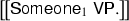
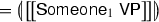
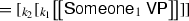
If we compute the denotation of [$_\mathsf{M }$Someone VP.] by the rules of Sect. 2.2, we obtain

No matter what VP is, the existential always scopes over it. Thus, we invariably get the linear-scope reading for the sentence. Obtaining the inverse-scope reading is the problem. One suggested solution (Barker 2002; de Groote 2001) is to introduce nondeterminism into semantic composition rules. We do not find that approach attractive because of over-generation: we may end up with a great number of denotations, not all of which correspond to available readings. Explaining different scope-taking abilities of existentials and universals (see Sect. 5) also becomes very difficult.

Our solution to inverse scope is the continuation hierarchy (Danvy and Filinski 1990). Like Russian dolls, contexts nest. Plugging a term into a context gives a bigger term, which can be plugged into another, wider context, and so on. This hierarchy of contexts is reflected in the continuation hierarchy. Quantifiers gain access not only to their immediate context but also to a higher-up context, and may hence quantify over outer contexts. We build the hierarchy from the CPS denotations of Sect. 2.2, to be called ${\mathrm {CPS}}^{1}$ denotations (with the annotated types of Sect. 3). We introduce the corresponding direct style of the hierarchy in Sect. 4.2.

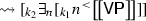
Before we begin, let us quickly skip ahead and peek at the final result, to see the difference that the continuation hierarchy makes. Equation (17) will look somewhat like

(see Eq. (25) for the complete example). VP will now have a chance to introduce a quantifier to scope over $\exists y.\cdot$.

We build the hierarchy by iterating the CPS transformation. An expression may be re-written in CPS multiple times. Each re-writing adds another continuation representing a higher (outer) context (Danvy and Filinski 1990). Let us take an example. A term $\mathbf{john }$ written in CPS takes the continuation argument representing the term’s context, and plugs itself into that context: $\mathopen {\lambda {k}.\,}k\ \mathbf{john }$. Mechanically applying to it the rules of transforming terms into CPS (Danvy and Filinski 1990) gives $\mathopen {\lambda {k_1}.\,}\mathopen {\lambda {k_2}.\,}(k_1\ \mathbf{john })\ k_2$. This ${\mathrm {CPS}}^{2}$ term receives two continuations and plugs $\mathbf{john }$ into the inner one, obtaining the ${\mathrm {CPS}}^{1}$ term $k_1\ \mathbf{john }$ that computes the result to be plugged into the outer context $k_2$. We may diagram the ${\mathrm {CPS}}^{1}$ term $\mathopen {\lambda {k_1}.\,}k_1\ \mathbf{john }$ as $[_{k_1} \ldots [\mathbf{john }] \ldots ]$, that is, $\mathbf{john }$ filling in the hole in a context represented by $k_1$. Likewise we diagram the ${\mathrm {CPS}}^{2}$ term $\mathopen {\lambda {k_1}.\,}\mathopen {\lambda {k_2}.\,}(k_1\ \mathbf{john })\ k_2$ as $[_{k_2} \ldots [_{k_1} \ldots [\mathbf{john }] \ldots ] \ldots ]$. In the ${\mathrm {CPS}}^{2}$ case, if $k_2$ represents the outer context, the application $k_2\ e$ represents plugging $e$ into that context. If $k_1$ is an inner context, $k_1\ e\ k_2$ corresponds to plugging $e$ into it and the result into an outer context $k_2$. We shall see soon that types make it clear which context, outer or inner, a continuation represents and what needs to be plugged into what.

The ${\mathrm {CPS}}^{2}$ term $\mathopen {\lambda {k_1}.\,}\mathopen {\lambda {k_2}.\,}k_1\ \mathbf{john }\ k_2$ is however extensionally equivalent to the ${\mathrm {CPS}}^{1}$ term $\mathopen {\lambda {k}.\,}k\ \mathbf{john }$ we started with. In general, if a term uses its continuation ‘trivially’,⁴ further CPS transformations leave the term intact. Thus, after quantifier-free lexical entries are converted once into CPS, they can be used as they are at any level of the CPS hierarchy.

Although the ${\mathrm {CPS}}^{2}$ term of $\mathbf{john }$ is same as the ${\mathrm {CPS}}^{1}$ term, the types differ. The ${\mathrm {CPS}}^{1}$ type is $(e\rightarrow t^n)\rightarrow t^n$, telling us that $\mathbf{john }$ receives a context to be plugged with a term of the type $e$ giving a term of the type $t^n$. The ${\mathrm {CPS}}^{2}$-term receives another continuation $k_2$, representing the outer context $t^{n}\rightarrow t^{l_1}$. Thus the type of $\mathopen {\lambda {k_1}.\,}\mathopen {\lambda {k_2}.\,}k_1\ \mathbf{john }\ k_2$ is $(e\rightarrow ((t^n\rightarrow t^{l_1})\rightarrow t^{l_2}))\rightarrow ((t^n\rightarrow t^{l_1})\rightarrow t^{l_2})$. This type is schematic, written with schematic meta-variables $n$, $l_1$ and $l_2$ standing for some variable names to be determined when building a derivation, as described in Sect. 3.

In general, types in the CPS hierarchy have a regular structure and can be described uniformly. The key observation is recurrence of the pattern $(t^n\rightarrow t^{l_1})\rightarrow t^{l_2}$ that can be represented by its sequence of annotations $n, l_1, l_2$. Therefore, we introduce the notation

• (18)

where all $n$s and $l$s are schematic meta-variables. Since these sequences can become very long, we use Greek letters $\alpha , \beta , \gamma$ to each stand for a schematic sequence of variable names. All occurrences of the same Greek letter bearing the same superscripts and subscripts refer to the same sequence. We will state the length of the sequence separately or leave it implicit in the CPS level under discussion. Thus the type of $\mathopen {\lambda {k}.\,}k\ \mathbf{john }$ for any CPS level has the form $(e\rightarrow \{\alpha \})\rightarrow \{\alpha \}$. Juxtaposed Greek letters and schematic variables signify concatenated sequences. For example, (18) is compactly written as follows.

• (19)

4.1 CPS-Hierarchy Semantics

The ${\mathrm {CPS}}^{2}$ semantics for our language fragment is shown in Fig. 10. Except for the quantifiers, the figure looks like the ordinary CPS semantics, Fig. 5, with the wholesale replacement of the type $t$ by $\{\alpha \}$. The interesting part is quantifier words. There are now two sets of them, indexed with $1$ and $2$: the quantifier words become polysemous, with two possible denotations. Postulating the polysemy of quantifiers is similar to generalizing the conjunction schema (Partee and Rooth 1983), or assuming the free indexing in LF.

The quantifiers everyone$_1$ and someone$_1$ are the quantifiers from Sect. 2.2, whose denotations are re-written in CPS. For example, the denotation of everyone from Fig. 9 (which is the precise version of that from Fig. 5) is $\mathopen {\lambda {k}.\,}\forall _n (k\ n)$; re-writing it in CPS gives $\mathopen {\lambda {k_1}.\,}\mathopen {\lambda {k_2}.\,}k_1\ n\ (\mathopen {\lambda {v}.\,}k_2 (\forall _n v))$. It plugs the variable $n$ into the (inner) context $k_1$, then plugs the result into $\forall _n[]$ and finally into the outer context $k_2$. Thus, everyone$_1$ quantifies over the immediate, inner context $k_1$, as in Sect. 2.2 above. The continuation arguments to everyone$_1$ are used trivially, so the denotation can be used as it is not only for ${\mathrm {CPS}}^{2}$ but also for ${\mathrm {CPS}}^{3}$ and at higher levels.

Fig. 10

Syntax and the ${\mathrm {CPS}}^{2}$ semantics for the small fragment. $\alpha$ and $\beta$ are sequences of schematic meta-variables of length 3, and $\gamma$ is a sequence of length 2. See the text for expressions and types of the semantic composition operators ${}^{>}$, ${}^{<}$ and $\mathopen {\left( \big \vert \right. } {\cdot } \mathclose {\left. \big \vert \right) }$

The second set of quantifiers quantify over the outer context, as their denotation says. For example, $\mathopen {\lambda {k_1}.\,}\mathopen {\lambda {k_2}.\,}\forall _n (k_1\ n\ k_2)$ plugs the variable $n$ into the inner context $k_1$, plugs the result into $k_2$ and quantifies over the final result. The inner and the outer contexts are uniquely determined, as shall see shortly.

The semantic combinators ${}^{>}$ and ${}^{<}$ in (10) use their continuation argument trivially; therefore, they also work for ${\mathrm {CPS}}^{2}$ and for all other levels of the hierarchy. We need to give them more general schematic types, extending Fig. 8 so it works at any level of the hierarchy:

• (20) $\frac{m_1 : (\sigma _2^{n_1}\rightarrow \{\alpha \})\rightarrow \{\beta \} \quad m_2 : ((\sigma _2\sigma _1)^{n_2}\rightarrow \{\gamma \})\rightarrow \{\alpha \}}{m_1{}^{<}m_2 : (\sigma _1^{\max (n_1,n_2)}\rightarrow \{\gamma \})\rightarrow \{\beta \}}$

• (21) $\frac{m_1 : ((\sigma _2\sigma _1)^{n_1}\rightarrow \{\alpha \})\rightarrow \{\beta \} \quad m_2 : (\sigma _2^{n_2}\rightarrow \{\gamma \})\rightarrow \{\alpha \}}{m_1{}^{>}m_2 : (\sigma _1^{\max (n_1,n_2)}\rightarrow \{\gamma \})\rightarrow \{\beta \}}$

We only need to change $\mathopen {\left( \big \vert \right. } {\cdot } \mathclose {\left. \big \vert \right) }$ to account for the two continuation arguments, and hence, two initial continuations:

• (22) $\mathopen {\left( \big \vert \right. } {m} \mathclose {\left. \big \vert \right) } \mathop {=}\limits ^{\text {def}}m (\mathopen {\lambda {v}.\,}\mathopen {\lambda {k_2}.\,}k_2\ v)(\mathopen {\lambda {v}.\,}v)$

The initial ${\mathrm {CPS}}^{1}$ continuation $(\mathopen {\lambda {v}.\,}\mathopen {\lambda {k_2}.\,}k_2\ v)$ plugs its argument into the outer context; the initial outer context is the empty context. Schematically, $\mathopen {\left( \big \vert \right. } {m} \mathclose {\left. \big \vert \right) }$ may be diagrammed as $[_{k_2} [_{k_1} m ]]$.

The two sets of quantifiers, level-1 and level-2, treat the inner and outer contexts differently. The remainder of this subsection presents several examples of computing denotations of sample sentences by using the lexical entries and the composition rules of Fig. 10 and performing simplifications by $\beta$-reductions. As we shall see, the sequence of reductions for, say, Someone$_1$VPcan be diagrammed at a high level as follows:

• (23)

We hence see that it is the level-1 quantifiers that wedge themselves between the inner context $k_1$ and the outer context $k_2$. We also see that, if the VP contains only level-1 QNPs, they would quantify over $[_{k_1} n {}^{<}\ldots ]$ giving the linear-scope reading. On the other hand, if the VP has a level-2 QNP, it will quantify over the outer context $[_{k_2} \exists _n [_{k_1} n {}^{<}\ldots ]]$ yielding the inverse-scope reading. After this preview, we describe the computation of denotations in detail.

It is a simple exercise to show that [$_\mathsf{M }$Someone$_1$ [$_\mathsf VP$saw everyone$_1$ ].] has the same linear-scope reading $\exists _0\forall _1 \mathbf{see }\cdot 1\cdot 0$ as computed with the ordinary CPS, Sect. 2.2—with essentially the same $\beta$-reductions shown in that section. It is also easy to see that [$_\mathsf{M }$Someone$_2$ [$_\mathsf VP$saw everyone$_2$ ].] also has exactly the same denotation. The interesting cases are the sentences with different levels of quantifiers. For example,

(1)

The result still shows the linear-scope reading, because someone$_2$ quantifies over the wide context and so wins over the narrow-context quantifier everyone$_1$. One may wonder how we chose the names of the quantified variables: $0$ for someone$_2$ and $1$ for everyone$_1$. The choice is clear from the final denotation: since it should have the type $t^0$ (that is, be closed), the schema for the corresponding someone$_2$ must have been instantiated with $n=0$. Therefore, $\forall _1 (\mathbf{see }\cdot 1\cdot 0)$ must have the type $t^1$, which determines the schema instantiation for everyone$_1$. One may say that ‘names follow scope’. The variable names can also be chosen before $\beta$-reducing, while building the typing derivation, as demonstrated in Sect. 3.

We now make a different choice of lexical entries for the same quantifier words in the running example:

(2)

We obtain the inverse-scope reading: everyone$_2$ quantified over the higher, or wider, context and hence outscoped someone$_1$. This outscoping is noticeable already in the result of the first set of $\beta$-reductions, which may be diagrammed as $\forall _0 [_{k_2} \exists _1 [_{k_1} \mathbf{see }\cdot 0\cdot [1]]]$. Since the universal quantifier eventually got the widest scope, the schema for everyone$_2$ must have been instantiated with $n=0$. Again, the choice of quantifier variable names is determined by quantifiers’ scope.

Thus the continuation hierarchy lets us derive both linear- and inverse-scope readings of ambiguous sentences. The source of the quantifier ambiguity is squarely in the lexical entries for the quantifier words rather than in the rules of syntactic formation or semantic composition.

4.2 Continuation Hierarchy in Direct Style

Like the ordinary CPS, the CPS hierarchy can also be built on demand. Therefore, we do not have to decide in advance the highest CPS level for our denotations, and be forced to rebuild our fragment’s denotations should a new example call for yet a higher level. Rather, we build sentence denotations by combining parts with different CPS levels, or even not in CPS. The primitive parts, lexical entry denotations, may remain not in CPS (which is the case for all quantifier-free entries) or at the minimum needed CPS level, regardless of the level of other entries. The incremental construction of hierarchical CPS denotations—building up levels only as required—makes our fragment modular and easy to extend. It also relieves us from the tedium of dealing with unnecessarily high-level CPS terms.

Luckily, the semantic combinators ${}^{<}$ and ${}^{>}$ capable of combining the denotations of different CPS levels have already been defined. They are (14) and (15) in Sect. 2.3. The luck comes from the fact that the composition of ${\mathrm {CPS}}^{1}$ denotations uses its continuation argument trivially, and therefore, works at any level of the CPS hierarchy. We only need to extend the schema for $\mathopen {\left( \big \vert \right. } {\cdot } \mathclose {\left. \big \vert \right) }$, in a regular way:

$$\begin{aligned} \mathopen {\left( \big \vert \right. } {m} \mathclose {\left. \big \vert \right) } \mathop {=}\limits ^{\text {def}}\left\{ \begin{array}{lll} m&{}\text {if}&{} m:\{0\}\\ m (\mathopen {\lambda {v}.\,}v) &{}\text {if}&{}m:\{nn0\}\\ m (\mathopen {\lambda {v}.\,}\mathopen {\lambda {k}.\,}kv) (\mathopen {\lambda {v}.\,}v) &{}\text {if}&{} m:\{nnl_1l_1l_2l_20\}\\ \ldots &{} &{} \end{array}\right. \end{aligned}$$

(3)

Applying the schematic definition (26) requires a bit of explanation. If the term $m$ has the type with no arrows, we should compute $\mathopen {\left( \big \vert \right. } {m} \mathclose {\left. \big \vert \right) }$ according to the first case, which requires $m$ be of the type $t^0$. If $m$ has the type that matches $\{nn0\}$, that is, $(t^n\rightarrow t^n)\rightarrow t^0$ for some $n$, we should use the second case, and so on. A term like $\mathopen {\lambda {k}.\,}k\ (\mathbf{leave }\cdot \mathbf{john })$ of the schematic type $\{0\alpha \alpha \}$ may seem confusing: its type matches $\{nn0\}$ (with $\alpha$ instantiated to $\{0\}$ and $n$ to $0$) as well as the type $\{nnl_1l_1l_2l_20\}$ (with $\alpha = \{000\}$ and $n=l_1=l_2=0$) and all further CPS types. We can compute $\mathopen {\left( \big \vert \right. } {\mathopen {\lambda {k}.\,}k\ (\mathbf{leave }\cdot \mathbf{john })} \mathclose {\left. \big \vert \right) }$ according to the second or any following case. The ambiguity is spurious however: whichever of the applicable equations we use, the result is the same—which follows from the fact that a ${\mathrm {CPS}}^{i}$ term which uses its continuation argument trivially is a ${\mathrm {CPS}}^{i'}$ term for all $i'\ge i$Danvy and Filinski (1990). As a practical matter, choosing the lowest-level instance of the schema (26) produces the cleanest derivation.

Figure 11 shows our new fragment.

Fig. 11

Syntax and the multi-level direct-style continuation semantics for the small fragment: the merger of Figs. 3, 10. Lexical entries other than the quantifiers keep the simple denotations from Fig. 3. Here $\alpha$, $\beta$ and $\gamma$ are sequences of schematic meta-variables whose length is determined by the CPS level; $\beta$ is two longer than $\gamma$

The quantifier-free lexical entries have the simplest denotations and can be combined with ${\mathrm {CPS}}^{n}$ terms, $n\ge 0$. The quantifiers everyone$_1$ and someone$_1$ have the schematic denotations that can be used at the ${\mathrm {CPS}}^{n}$ level $n\ge 1$. The higher-level quantifiers are systematically produced by applying the $\uparrow$ combinator of the type $((e^{n+1}\rightarrow \{\alpha \})\rightarrow \{\beta \}) \rightarrow ((e^{n+1}\rightarrow \{\gamma \alpha \})\rightarrow \{\gamma \beta \})$ (where $\alpha$ and $\beta$ have the same length and $\gamma$ is one longer).

• (27) $\uparrow m \mathop {=}\limits ^{\text {def}}\mathopen {\lambda {k}.\,}\mathopen {\lambda {k'}.\,}m (\mathopen {\lambda {v}.\,}k\ v\ k')$

With the entries in Fig. (11), all sample derivations from Sect. 4 can be repeated in direct style with hardly any changes.

Our direct-style multi-level continuation semantics is essentially the same as that presented in Shan (2004). We do not account for directionality in semantic types (since we use CFG or potentially CCG, rather than type-logical grammars) but we do account for the levels of quantified variables in types (whereas in Shan (2004), quantification was handled informally).

We have thus shown that the CPS hierarchy just as the ordinary CPS can be built on demand, without committing ourselves to any particular hierarchy level but raising the level if needed as a denotation is being composed. The result is the modular semantics, and much simpler and more lucid semantic derivations. From now on, we will use this multi-level direct style.

5 Scope Islands and Quantifier Strength

We have used the continuation hierarchy to explain quantifier ambiguity between linear- and inverse-scope readings. We contend that the ambiguity arises because quantifier words are polysemous: they have multiple denotations corresponding to different levels of the CPS hierarchy. The higher the CPS level, the wider the quantifier scope.

We turn to two further problems. First, just quantifiers’ competing with each other on their strength (CPS level) does not explain all empirical data. Some syntactic constructions such as embedded clauses come into play and restrict the scope of embedded quantifiers. That restriction however does not seem to spread to indefinites: “the varying scope of indefinites is neither an illusion nor a semantic epiphenomenon: it needs to be ‘assigned’ in some way” (Szabolcsi 2000). We shall use the CPS hierarchy to account for scope islands and to assign the varying scope to indefinites.

5.1 Scope Islands

Like our running example “Someone saw everyone”, two characteristic examples (4) and (5), repeated below, also have two quantifier words.

• (28) That every boy left upset a teacher.

• (29) Someone reported that John saw everyone.

These examples are not ambiguous however: (28) (the same as (4)) has only the inverse-scope reading, whereas (29) (the same as (5)) has only the linear-scope reading. The common explanation (see survey Szabolcsi (2000)) is that embedded tensed clauses are scope islands, preventing embedded quantifiers from taking scope wider than the island.

To analyze these examples, we at least have to extend our fragment with more lexical entries and with syntactic forms for clausal NPs, with the corresponding semantic combinators.⁵ Figure 12 shows the additions. Most of them are straightforward. In particular, we generalize quantifying NPs like everyone to quantifying determiners like every. The determiner receives an extra $(et)$ argument for its restrictor property, of the type of the denotation of a common noun.⁶ Unlike Barker (2002), we do not use choice functions in the denotations for the quantifier determiners. Instead, the denotation of the NP is obtained from the denotations of the Det and N by ordinary function application.

Fig. 12

Syntax and the multi-level direct-style continuation semantics for the additional fragment

Just as quantifying NPs are polysemous, so are quantifying Dets on our analysis: there are weak (or level-1) forms every$_1$ and a$_1$ and strong (or level-2) forms every$_2$ and a$_2$. Stronger quantifiers outscope weaker ones. For example, [$_\mathsf{M }$ [$_\mathsf S$ [a$_1$boy] [upset [every$_2$teacher]]].] determines the inverse-scope reading $\forall _0(\mathbf{teacher }\cdot 0 \implies \exists _1 (\mathbf{boy }\cdot 1 \wedge \mathbf{upset }\cdot 0\cdot 1))$.

Recall from Fig. 11 how the matrix denotation $\mathsf{M }\rightarrow \mathsf S .$ is obtained from the denotation of the main clause: $\left[ \left[ \mathsf{M }\right] \right] =\mathopen {\left( \big \vert \right. } {\left[ \left[ \mathsf S \right] \right] } \mathclose {\left. \big \vert \right) }$. We see exactly the same pattern for the clausal NPs in the semantic operations corresponding to $\mathsf Vs \ \mathsf that \ \mathsf S$ and $\mathsf that \ \mathsf S$: in all the cases, the denotation of a clause is enclosed within $\mathopen {\left( \big \vert \right. } {\cdot } \mathclose {\left. \big \vert \right) }$, which is the semantic counterpart of the syntactic clause boundary. The typing rules for $\mathopen {\left( \big \vert \right. } {\cdot } \mathclose {\left. \big \vert \right) }$ in Fig. 8 specify its result have the type $t^0$, as befits the denotation of a clause. The type $t^0$ is not a CPS type and hence $\mathopen {\left( \big \vert \right. } {\left[ \left[ \mathsf S \right] \right] } \mathclose {\left. \big \vert \right) }$ cannot get hold of its context to quantify over. Therefore, if S had any embedded quantifiers, they can quantify only as far as the clause. The operation $\mathopen {\left( \big \vert \right. } {\cdot } \mathclose {\left. \big \vert \right) }$ thus acts as the scope delimiter, delimiting the context over which quantification is possible. (Incidentally, the same typing rules of $\mathopen {\left( \big \vert \right. } {\cdot } \mathclose {\left. \big \vert \right) }$ severely restrict how this scope-delimiting operation may be used within lexical entries. For example, $\mathopen {\left( \big \vert \right. } {\left[ \left[ \mathsf VP \right] \right] } \mathclose {\left. \big \vert \right) }$ is ill-typed since VP does not have the type $t^n$ or $(t^n\rightarrow \{\alpha \})\rightarrow \{\beta \}$.)

In case of (28), we obtain the same denotation (30) no matter which lexical entry we choose for the embedded determiner, $\mathsf{every }_1$ (31) or $\mathsf{every }_2$ (32). The quantifier remains trapped in the clause and the sentence is not ambiguous. Incidentally, since all quantifier variables used within a clause will be quantified within the clause, their names can be chosen regardless of the names of other variables within the sentence. That’s why the name $0$ is reused in (30). Again, names follow scope. A similar analysis applies to (29).

• (30) $\exists _0 (\mathbf{teacher }\cdot 0 \wedge \mathbf{upset }\cdot 0\cdot (\mathbf{That }\cdot \forall _0 (\mathbf{boy }\cdot 0 \implies \mathbf{leave }\cdot 0)))$

• (31)

• (32)

We have demonstrated that a scope island is an effect of the operation $\mathopen {\left( \big \vert \right. } {\cdot } \mathclose {\left. \big \vert \right) }$, which is the semantic counterpart of the syntactic clause boundary. In our analysis, each surface syntactic constituent still corresponds to a well-formed denotation, and each surface syntactic formation rule still corresponds to a semantic combinator. Our approach hence is directly compositional.

5.2 Wide-Scope Indefinites

Given that enclosing all clause denotations in $\mathopen {\left( \big \vert \right. } {\cdot } \mathclose {\left. \big \vert \right) }$ traps all quantifiers inside, how do indefinites manage to get out? And they do get out: “Indefinites acquire their existential scope in a manner that does not involve movement and is essentially syntactically unconstrained” (Szabolcsi 2000, Sect. 3.2.1). For example:

• (33) $\text {Everyone reported that [Max and some lady] disappeared.}$

• (34) $\text {Most guests will be offended [if we don't invite some philosopher].}$

• (35) $\text {All students believe anything [that many teachers say].}$

Szabolcsi argued (Szabolcsi 2000) that all these examples are ambiguous. In particular, in (33) (the same as (7)), either different people meant a different lady disappearing along with Max, or there is one lady that everyone reported as disappearing along with Max. Interestingly, the example

• (36) Someone reported that [Max and every lady] disappeared.

is not ambiguous: there is a single reporter of the disappearance for Max and all ladies. The unambiguity of (36) is explained by the embedded clause’s being a scope island, which prevents the universal from taking wide scope. The ambiguity of (33) leads us to conclude that indefinites, in contrast to universals, can scope out of clauses, complements and coordination structures. Szabolcsi (2000) gives a large amount of evidence for this conclusion. Accordingly, our theory must first explain how anything can get out of a scope island, then postulate that only indefinites have this escaping ability.

The operation $\mathopen {\left( \big \vert \right. } {\cdot } \mathclose {\left. \big \vert \right) }$ that effects the scope island has the schematic type that can be informally depicted as ${\mathrm {CPS}}^{i}[t]\rightarrow {\mathrm {CPS}}^{0}[t]$ where

$$\begin{aligned} {\mathrm {CPS}}^{i}[t] = \{\alpha \} \quad \text {where the length of} \,\alpha \, \mathrm{{is}} \, 2^{i+1}-1 \end{aligned}$$

Since the result of $\mathopen {\left( \big \vert \right. } {m} \mathclose {\left. \big \vert \right) }$ has a ${\mathrm {CPS}}^{0}$ type, that is $t$, the result cannot get hold of any context. Hence we need a less absolutist version of $\mathopen {\left( \big \vert \right. } {\cdot } \mathclose {\left. \big \vert \right) }$ which merely lowers rather than collapses the hierarchy. We call that operation $\mathopen {\left( \big \vert \right. } {\cdot } \mathclose {\left. \big \vert \right) }_2$, of the informal schematic type ${\mathrm {CPS}}^{\le 2}[t]\rightarrow {\mathrm {CPS}}^{0}[t]$ and ${\mathrm {CPS}}^{i+2}[t]\rightarrow {\mathrm {CPS}}^{i}[t]$ where $i\ge 1$. Whereas $\mathopen {\left( \big \vert \right. } {m} \mathclose {\left. \big \vert \right) }$ delimits all the contexts of $m$, $\mathopen {\left( \big \vert \right. } {m} \mathclose {\left. \big \vert \right) }_2$ delimits only the first two contexts of the hierarchy. Quantifiers within $m$ of level 3 and higher will be able to get hold of the context of $\mathopen {\left( \big \vert \right. } {m} \mathclose {\left. \big \vert \right) }_2$. One may think of $\mathopen {\left( \big \vert \right. } {\cdot } \mathclose {\left. \big \vert \right) }_2$ as the inverse of $\uparrow \uparrow$. The following example illustrates the lowering:

• (37a) $\left[ \left[ \mathsf{someone_1~left }\right] \right] = \mathopen {\lambda {k_1}.\,}\mathopen {\lambda {k_2}.\,} k_1\ (\mathbf{leave }\cdot n)\ (\mathopen {\lambda {v}.\,}k_2 \exists _nv)$

• (37b) $\mathopen {\left( \big \vert \right. } {\left[ \left[ \mathsf{someone _1~\mathsf{left }}\right] \right] } \mathclose {\left. \big \vert \right) }_2 = \exists _0(\mathbf{leave }\cdot 0)$

• (37c) $\mathopen {\left( \big \vert \right. } {\uparrow \left[ \left[ \mathsf{someone _1~\mathsf{left }}\right] \right] } \mathclose {\left. \big \vert \right) }_2 = \exists _0(\mathbf{leave }\cdot 0)$

• (37d) $\mathopen {\left( \big \vert \right. } {\uparrow \uparrow \left[ \left[ \mathsf{someone _1~\mathsf{left }}\right] \right] } \mathclose {\left. \big \vert \right) }_2 = \mathopen {\lambda {k_1}.\,}\mathopen {\lambda {k_2}.\,} k_1\ (\mathbf{leave }\cdot n)\ (\mathopen {\lambda {v}.\,}k_2 \exists _nv)$

In (37a) and the identical (37d), the existential quantifies over the potentially wide context $k_1$. In (37b) and (37c), whose denotations are again identical, $\exists _0$ scopes just over $\mathbf{leave }\cdot 0$ and extends no further.

Why did we choose 2 as the number of contexts to delimit at the embedded clause boundary? Any number $i\ge 2$ will work, to explain the quantifier ambiguity within the embedded clause and wide-scope indefinites. We chose $i=2$ for now pending analysis of more empirical data.

If (37a)–(37d) is the specification for $\mathopen {\left( \big \vert \right. } {\cdot } \mathclose {\left. \big \vert \right) }_2$, then (38) below is the implementation. It is derived from the schema (26) by cutting it off after the third line and inserting the generic lowering-by-two operation as the final default case.

$$\begin{aligned} \mathopen {\left( \big \vert \right. } {m} \mathclose {\left. \big \vert \right) }_2 \mathop {=}\limits ^{\text {def}}{\left\{ \begin{array}{ll} m &{}\text {if}~m:\{0\}\\ m (\mathopen {\lambda {v}.\,}v) &{}\text {if}~m:\{nn0\}\\ m (\mathopen {\lambda {v}.\,}\mathopen {\lambda {k}.\,}kv) (\mathopen {\lambda {v}.\,}v) &{}\text {if}~m:\{nnl_1l_1l_2l_20\}\\ m (\mathopen {\lambda {v}.\,}\mathopen {\lambda {k}.\,}kv) (\mathopen {\lambda {v}.\,}\mathopen {\lambda {k}.\,}kv) &{}\text {otherwise} \end{array}\right. } \end{aligned}$$

(4)

It is easy to show that the definition (38) indeed satisfies (37a)–(37d). A useful lemma is the identity $(\uparrow m) (\mathopen {\lambda {v}.\,}\mathopen {\lambda {k}.\,}kv) = m$, easily verified from the definition (27) of $\uparrow$.

To make use of this lowering operation $\mathopen {\left( \big \vert \right. } {\cdot } \mathclose {\left. \big \vert \right) }_2$, we adjust the lexical entries in Fig. 12 as shown in Fig. 13. The main change is replacing $\mathopen {\left( \big \vert \right. } {\cdot } \mathclose {\left. \big \vert \right) }$ in the semantic composition rules for embedded clauses with $\mathopen {\left( \big \vert \right. } {\cdot } \mathclose {\left. \big \vert \right) }_2$. In other words, we now distinguish the main clause boundary from embedded clause boundaries. Figure 13 also reflects our postulate: only indefinites may be at the CPS level 3 and higher—not universals.

Fig. 13

Adjustments to the syntax and the multi-level direct-style continuation semantics for the additional fragment, to account for wide-scope indefinites. If the size of the sequence $\gamma$ is $j$, the size of $\beta _3$ is $3(j+2)$ and of $\beta _4$ is $7(j+2)$

The typical example (33) can now be analyzed as follows (see Fig. 12 for the denotations of disappeared and report):

• (39) $[_\mathsf{M }\,\mathsf{Everyone }_1 \mathsf{reported that }\,[_\mathsf S \, \mathsf{Max and some }_\mathsf{i }\, \mathsf{lady disappeared }].]$

When the level $i$ of $\mathsf{some }_\mathsf{i }$ is $1$ or $2$, the indefinite is trapped in the scope island.

• (40a) $\forall _0 \mathbf{report }\cdot \left( \exists _0 (\mathbf{lady }\cdot 0 \wedge \mathbf{disappear }\cdot (\mathbf{alongWith }\cdot \mathbf{max }\cdot 0))\right) \cdot 0$

At the level $i=3$, the indefinite scopes out of the clause but is defeated by the universal in the subject position, giving us another linear-scope reading, along the lines expounded in Sect. 2.2.

• (40b) $\forall _{0}\exists _1 \mathbf{lady }\cdot 1 \wedge \mathbf{report }\cdot (\mathbf{disappear }\cdot (\mathbf{alongWith }\cdot \mathbf{max }\cdot 1))\cdot 0$

Finally, $\mathsf{some }_4$, lowered from level 4 to level 2 as it crosses the embedded clause boundary, has sufficient strength left to scope over the entire sentence.

• (40c) $\exists _0\mathbf{lady }\cdot 0 \wedge \forall _1\mathbf{report }\cdot (\mathbf{disappear }\cdot (\mathbf{alongWith }\cdot \mathbf{max }\cdot 0)) \cdot 1$

5.3 Inverse Linking

Our analysis of inverse linking turns out quite similar to the analysis of wide-scope indefinites. We take the argument NP of a PP to be a scope island, albeit it is evidently a weaker island than an embedded tensed clause. We realize the island by an operation similar to $\mathopen {\left( \big \vert \right. } {\cdot } \mathclose {\left. \big \vert \right) }_2$. Therefore, a strong enough quantifier embedded in NP can escape and take a wide scope. That escaping from the island corresponds to inverse linking.

To demonstrate our analysis, we extend our fragment with prepositional phrases; see Fig. 14. We add a category of N’ of nouns adjoined with PP. We generalize Det to take as its argument N’ rather than bare common nouns. For simplicity, we use the same $\mathopen {\left( \big \vert \right. } {\cdot } \mathclose {\left. \big \vert \right) }_2$ operation for the PP island as we used for the embedded-clause island. Recall that $(\wedge )$ is a constant of the type $t(tt)$ and we write the $\mathcal {D}_Q$ expression $(\wedge )\cdot d_1\cdot d_2$ as $d_1 \wedge d_2$.

Fig. 14

Adjustments to the syntax and the multi-level direct-style continuation semantics for the additional fragment, to account for prepositional phrases. The higher-level quantificational determiners are produced with the $\uparrow$ operations; see Fig. 13 for illustration. If the size of the sequence $\alpha$ is $j$, the size of $\beta$ is also $j$ and the size of $\gamma$ is $2j+1$

The type of the quantificational determiners shows that a determiner takes a restrictor and a continuation, which may contain $n$ other free variables. The determiner adds a new one, which it then binds. Although the denotations of determiners in Fig. 14 bind the variables they themselves introduced, that property is not assured by the type system. For example, nothing prevents us from writing ‘bad’ lexical entries like $\mathopen {\lambda {z}.\,} \forall _n z$ or $1$. Although the type system will ensure that the overall denotation is closed, what a binder ends up binding will be hard to predict. It is an interesting problem to define ‘good’ lexical entries (with respect to scope) and codify the notion in the type system. This is the subject of ongoing work Kameyama et al. (2011).

We analyze inverse linking thusly.

• (41a) ${[ _\mathsf{NP }\,\mathsf{No } [ _\mathsf{N' }\,[ _\mathsf{N' }\, \mathsf{man }] [ _\mathsf{PP }\,\mathsf{from a foreign }\, \mathsf{country }]]]} \mathsf{was admitted }.$

• (41b) $neg\cdot \exists _0\mathbf{man }\cdot 0 \wedge (\exists _1 \mathbf{country }\cdot 1 \wedge \mathbf{from }\cdot 1\cdot 0) \wedge \mathbf{admitted }\cdot 0$

• (41c) $exists_0\mathbf{country }\cdot 0 \wedge \lnot \cdot \exists _1 \mathbf{man }\cdot 1 \wedge \mathbf{from }\cdot 0\cdot 1 \wedge \mathbf{admitted }\cdot 1$

The PP in (41a) contains an ambiguous quantifier. If the quantifier is weak, it is trapped in the PP island and gives the salient reading (41b). If the quantifier is strong enough to escape, the inverse-linking reading (41c) emerges. We thus reproduce quantifier ambiguity for QNP within NP and explain inverse linking.

6 Conclusions

We have given the first rigorous account of linear- and inverse-scope readings, scope islands, wide-scope indefinites and inverse linking based on the D&F continuation hierarchy. Quantifier ambiguity arises because quantifier words are polysemous, with multiple denotations corresponding to different levels of the hierarchy. The higher the level, the wider the scope. Embedded clauses and PPs create scope islands by lowering the hierarchy and trapping low-level quantifiers. Higher-level quantifiers (which we postulate only indefinites possess) can escape the island and take wider scope. The continuation hierarchy lets us assign scope to indefinites and universals and explain their differing scope-taking abilities.

Our analysis is directly compositional: each surface syntactic constituent corresponds to a well-formed denotation, and each surface syntactic formation rule corresponds to a unique semantic combinator.

We have shown how to build the continuation hierarchy modularly and on-demand, without committing ourselves to any particular hierarchy level but raising the level if needed as a denotation is being composed. In particular, quantifier-free lexical entries have unlifted types and simple denotations.

We look forward to extending our analysis to other aspects of scope—how quantifiers interact with coordination (as in (1.1)), pronouns and polarity items—and to distributivity in universal quantification. We would also like to investigate if hierarchy levels can be correlated with Minimalism features or feature domains. Finally, we plan to extend our analyses of single sentences to discourse.

References

Barker, C. (2002). Continuations and the nature of quantification. Natural Language Semantics, 10(3), 211–242.
Barker, C., & Shan, C.-c. (2006). Types as graphs: Continuations in type logical grammar. Journal of Logic, Language and Information, 15(4), 331–370.
Barker, C., & Shan, C.-c. (2008). Donkey anaphora is in-scope binding. Semantics and Pragmatics1(1), 1–46.
Bekki, D., & Asai, K. (2009). Representing covert movements by delimited continuations. Proceedings of the \(6{\text{ th }}\)International Workshop on Logic and Engineering of Natural Language Semantics, Japanese Society of, Artificial Intelligence (November 2009).
Bernardi, R., & Moortgat, M. (2010). Continuation semantics for the Lambek-Grishin calculus. Information and Computation, 208(5), 397–416.
Champollion, L., Tauberer, J., & Romero, M. (2007). The Penn Lambda Calculator: Pedagogical software for natural language semantics. In T. H. King & E. M. Bender (Eds.), Proceedings of the Workshop on Grammar Engineering Across Frameworks (pp. 106–127). Stanford: CA, Center for the Study of Language and Information.
Danvy, O., & Filinski, A. (1990). Abstracting control. Proceedings of the 1990 ACM Conference on Lisp and Functional Programming (pp. 151–160), New York, ACM Press (27–29 June 1990).
de Groote, P. (2001). Type raising, continuations, and classical logic. In R. van Rooy & M. Stokhof (Eds.), Proceedings of the \(13{\text{ th }}\)Amsterdam Colloquium (pp. 97–101). Institute for Logic: Language and Computation, Universiteit van Amsterdam.
Kameyama, Y., Kiselyov, O., & Shan, C.-c. (2011). Computational effects across generated binders: Maintaining future-stage lexical scope. Technical Report CS-TR-11-17, Department of Computer Science, Graduate School of Systems and Information Engineering, University of Tsukuba.
Montague, R. (1974). The proper treatment of quantification in ordinary English. In R. H. Thomason (Ed.), Formal philosophy: Selected papers of Richard Montague (pp. 247–270). New Haven: Yale University Press.
Partee, B. H., & Rooth, M. (1983). Generalized conjunction and type ambiguity. In R. Bäuerle, C. Schwarze, & A. von Stechow (Eds.), Meaning use and interpretation of language (pp. 361–383). Berlin: Walter de Gruyter.
Reinhart, T. (1979). Syntactic domains for semantic rules. In F. Guenthner & S. J. Schmidt (Eds.), Formal semantics and pragmatics for natural languages (pp. 107–130). Dordrecht: Reidel.
Rompf, T., Maier, I., & Odersky, M. (2009). Implementing first-class polymorphic delimited continuations by a type-directed selective CPS-transform. In G. Hutton & A. P. Tolmach (Eds.), ICFP ’09: Proceedings of the ACM International Conference on Functional Programming (pp. 317–328). New York: ACM Press.
Shan, C.-c. (2004). Delimited continuations in natural language: Quantification and polarity sensitivity. In H. Thielecke (Ed.), CW’04: Proceedings of the \(4{\text{ th }}\)ACM SIGPLAN Continuations Workshop (pp. 55–64). Number CSR-04-1 in Technical Report, School of Computer Science, University of Birmingham.
Shan, C.-c. (2007a). Linguistic side effects. In C. Barker & P. Jacobson (Eds.). Direct compositionality (pp. 132–163). New York: Oxford University Press.
Shan, C.-c. (2007b). Inverse scope as metalinguistic quotation in operational semantics. In: K. Yoshimoto (Ed.), Proceedings of the \(4{\text{ th }}\)International Workshop on Logic and Engineering of Natural Language Semantics (pp. 167–178), Japanese Society of Artificial Intelligence (18–19 June 2007).
Szabolcsi, A. (2000). The syntax of scope. In M. Baltin & C. Collins (Eds.), Handbook of contemporary syntactic theory (pp. 607–634). Oxford: Blackwell.
Szabolcsi, A. (2009). Quantification. Cambridge: Cambridge University Press.
Acknowledgments
We are very grateful to Chris Tancredi for many helpful suggestions and a thought-provoking conversation. We thank anonymous reviewers for their comments.
Author information
Authors and Affiliations
Corresponding author
Editor information
Editors and Affiliations
Rights and permissions
Copyright information
© 2014 Springer Science+Business Media Dordrecht
About this chapter
Cite this chapter
Kiselyov, O., Shan, Cc. (2014). Continuation Hierarchy and Quantifier Scope. In: McCready, E., Yabushita, K., Yoshimoto, K. (eds) Formal Approaches to Semantics and Pragmatics. Studies in Linguistics and Philosophy, vol 95. Springer, Dordrecht. https://doi.org/10.1007/978-94-017-8813-7_6
Download citation
DOI: https://doi.org/10.1007/978-94-017-8813-7_6
Publisher Name: Springer, Dordrecht
Print ISBN: 978-94-017-8812-0
Online ISBN: 978-94-017-8813-7
eBook Packages: Humanities, Social Sciences and LawSocial Sciences (R0)