Markov Model Theory

Abstract

This section reviews the relation between the continuous dynamics of a molecular system in thermal equilibrium and the kinetics given by a Markov State Model (MSM). We will introduce the dynamical propagator, an error-less, alternative description of the continuous dynamics, and show how MSMs result from its discretization. This allows for an precise understanding of the approximation quality of MSMs in comparison to the continuous dynamics. The results on the approximation quality are key for the design of good MSMs. While this section is important for understanding the theory of discretization and related systematic errors, practitioners wishing only to learn how to construct MSMs may skip directly to the discussion of Markov model estimation.

Part of this chapter is reprinted with permission from Prinz et al. (Markov models of molecular kinetics: Generation and validation. J. Chem. Phys. 134:174,105, 2011). Copyright 2011, American Institute of Physics.

A more detailed text book version is to be found in Schütte and Sarich (Metastability and Markov State Models in Molecular Dynamics: Modeling, Analysis, Algorithmic Approaches. Courant Lecture Notes, 24. American Mathematical Society, 2013).

These keywords were added by machine and not by the authors. This process is experimental and the keywords may be updated as the learning algorithm improves.

3.1 Continuous Molecular Dynamics

A variety of simulation models that all yield the same stationary properties, but have different dynamical behaviors, are available to study a given molecular model. The choice of the dynamical model must therefore be guided by both a desire to mimic the relevant physics for the system of interest (such as whether the system is allowed to exchange energy with an external heat bath during the course of dynamical evolution), balanced with computational convenience (e.g. the use of a stochastic thermostat in place of explicitly simulating a large external reservoir) [8]. Going into the details of these models is beyond the scope of the present study, and therefore we will simply state the minimal physical properties that we expect the dynamical model to obey. In the following we pursue the theoretical outline from Ref. [31] (Sects. 3.1–3.7) and Ref. [37] (Sects. 3.1–3.8) which should both be used for reference purposes.

Consider a state space Ω which contains all dynamical variables needed to describe the instantaneous state of the system. Ω may be discrete or continuous, and we treat the more general continuous case here. For molecular systems, Ω usually contains both positions and velocities of the species of interest and surrounding bath particles. x(t)∈Ω will denote the state of the system at time t. The dynamical process considered is $(\mathbf {x}(t))_{t\in T}, T \subset\mathbb{R}_{0+}$, which is continuous in space, and may be either time-continuous (for theoretical investigations) or time-discrete (when considering time-stepping schemes for computational purposes). For the rest of the article, the dynamical process will also be denoted by x(t) for the sake of simplicity; we assume that x(t) has the following properties:

• 1. x(t) is a Markov process in the full state space Ω, i.e. the instantaneous change of the system (d x(t)/dt in time-continuous dynamics and x(t+Δt) in time-discrete dynamics with time step Δt), is calculated based on x(t) alone and does not require the previous history. In addition, we assume that the process is time-homogeneous, such that the transition probability density p(x,y;τ) for x,y∈Ω and $\tau\in\mathbb{R}_{0+}$ is well-defined:

  $$\begin{aligned} p(\mathbf{x},A;\tau) = \mathbb{P}\bigl[\mathbf{x}(t+\tau)\in A\bigm| \mathbf{x}(t)=\mathbf{x} \bigr] \end{aligned}$$

  (3.1)

  i.e. the probability that a trajectory started at time t from the point x∈Ω will be in set A at time t+τ. Such a transition probability density for the diffusion process in a one-dimensional potential is depicted in Fig. 3.1b. Whenever p(x,A;τ) has an absolutely continuous probability density p(x,y;τ) it is given by integrating the transition probability density over region A:

  $$\begin{aligned} p(\mathbf{x},A;\tau) & = \mathbb{P}\bigl[\mathbf{x}(t+\tau)\in A\bigm| \mathbf{x}(t)=\mathbf{x} \bigr] \end{aligned}$$

  (3.2)
  $$\begin{aligned} & = \int_{A}d\mathbf{y}\,p(\mathbf{x},\mathbf{y};\tau). \end{aligned}$$

  (3.3)

  Fig. 3.1

  

  (a) Potential energy function with four metastable states and corresponding stationary density μ(x). (b) Density plot of the transfer operator for a simple diffusion-in-potential dynamics defined on the range Ω=[0,100], black and red indicates high transition probability, white zero transition probability. Of particular interest is the nearly block-diagonal structure, where the transition density is large within blocks allowing rapid transitions within metastable basins, and small or nearly zero for jumps between different metastable basins. (c) The four dominant eigenfunctions of the transfer operator, ψ ₁,…,ψ ₄, which indicate the associated dynamical processes. The first eigenfunction is associated to the stationary process, the second to a transition between A+B↔C+D and the third and fourth eigenfunction to transitions between A↔B and C↔D, respectively. (d) The four dominant eigenfunctions of the transfer operator weighted with the stationary density, ϕ ₁,…,ϕ ₄. (e) Eigenvalues of the transfer operator, The gap between the four metastable processes (λ _i ≈1) and the fast processes is clearly visible

• 2. x(t) is ergodic, i.e., the process x(t) is aperiodic, the space Ω does not have two or more subsets that are dynamically disconnected, and for t→∞ each state x will be visited infinitely often. The running average of a function $f:\varOmega \rightarrow\mathbb{R}^{d}$ then is given by a unique stationary density μ(x) in the sense that for almost every initial state x we have

  $$\lim_{T\to\infty}\frac{1}{T}\int_0^T dt\,f\bigl(\mathbf{x}(t)\bigr) = \int_\varOmega d\mathbf{x}\,f( \mathbf{x})\mu(\mathbf{x}), $$

  that is, the fraction of time that the system spends in any of its states during an infinitely long trajectory is given by the stationary density (invariant measure) $\mu(\mathbf{x}):\varOmega\rightarrow\mathbb{R}_{0+}$ with ∫ _Ω d x μ(x)=1, where the stationarity of the density means that

  $$\int_A d\mathbf{x}\,\mu(\mathbf{x}) = \int _\varOmega d\mathbf{x}\, p(\mathbf{x},A;\tau)\mu (\mathbf{x}), $$

  which takes the simpler form

  $$\mu(\mathbf{y}) = \int_\varOmega d\mathbf{x}\,p(\mathbf{x}, \mathbf {y};\tau)\mu(\mathbf{x}), $$

  whenever the transition probability has a density. We assume that this stationary density μ is unique. In cases relevant for molecular dynamics the stationary density always corresponds to the equilibrium probability density for some associated thermodynamic ensemble (e.g. NVT, NpT). For molecular dynamics at constant temperature T, the dynamics above yield a stationary density μ(x) that is a function of T, namely the Boltzmann distribution

  $$ \mu(\mathbf{x})=Z(\beta)^{-1}\exp \bigl(-\beta H(\mathbf{x}) \bigr) $$

  (3.4)

  with Hamiltonian H(x) and β=1/k _B T where k _B is the Boltzmann constant and k _B T is the thermal energy. Z(β)=∫d x exp(−βH(x)) is the partition function. By means of illustration, Fig. 3.1a shows the stationary density μ(x) for a diffusion process on a potential with high barriers.

• 3. x(t) is reversible, i.e., p(x,y;τ) fulfills the condition of detailed balance:

  $$ \mu(\mathbf{x}) p(\mathbf{x},\mathbf{y};\tau)=\mu(\mathbf {y}) p(\mathbf{y}, \mathbf{x};\tau ), $$

  (3.5)

  i.e., in equilibrium, the fraction of systems transitioning from x to y per time is the same as the fraction of systems transitioning from y to x. Note that this “reversibility” is a more general concept than the time-reversibility of the dynamical equations e.g. encountered in Hamiltonian dynamics. For example, Brownian dynamics on some potential are reversible as they fulfill Eq. (3.5), but are not time-reversible in the same sense as Hamiltonian dynamics are, due to the stochasticity of individual realizations. Although detailed balance is not essential for the construction of Markov models, we will subsequently assume detailed balance as this allows much more profound analytical statements to be made, and just comment on generalizations here and there. The rationale is that one typically expects detailed balance to be fulfilled in equilibrium molecular dynamics based on a simple physical argument: For dynamics that have no detailed balance, there exists a set of states which form a loop in state space which is traversed in one direction with higher probability than in the reverse direction. This means that one could design a machine which uses this preference of direction in order to produce work. However, a system in equilibrium is driven only by thermal energy, and conversion of pure thermal energy into work contradicts the second law of thermodynamics. Thus, this argument concludes that equilibrium molecular dynamics must be reversible and fulfill detailed balance. Despite the popularity of this argument there are dynamical processes used in molecular dynamics that do not satisfy detailed balance in the above sense. Langevin molecular dynamics may be the most prominent example. However, the Langevin process exhibits an extended detailed balance [18]

  $$\mu(\mathbf{x}) p(\mathbf{x},\mathbf{y};\tau)=\mu(A\mathbf {y}) p(A \mathbf{y},A\mathbf{x};\tau ),$$

  where A is the linear operation that flips the sign of the momenta in the state x. This property allows to reproduce the results for processes with detailed balance to this case, see remarks below.

The above conditions do not place overly burdensome restrictions on the choices of dynamical models used to describe equilibrium dynamics. Many stochastic thermostats are consistent with the above assumptions, e.g. Hybrid Monte Carlo [14, 37], overdamped Langevin (also called Brownian or Smoluchowski) dynamics [15, 16], and stepwise-thermalized Hamiltonian dynamics [42]. When simulating solvated systems, a weak friction or collision rate can be used; this can often be selected in a manner that is physically motivated by the heat conductivity of the material of interest and the system size [1].

We note that the use of finite-timestep integrators for these models of dynamics can sometimes be problematic, as the phase space density sampled can differ from the density desired. Generally, integrators based on symplectic Hamiltonian integrators (such as velocity Verlet [42]) offer greater stability for our purposes.

While technically, a Markov model analysis can be constructed for any choice of dynamical model, it must be noted that several popular dynamical schemes violate the assumptions above, and using them means that one is (currently) doing so without a solid theoretical basis, e.g. regarding the boundedness of the discretization error analyzed in Sect. 3.3 below. For example, Nosé-Hoover and Berendsen are either not ergodic or do not generate the correct stationary distribution for the desired ensemble [10]. Energy-conserving Hamiltonian dynamics on one hand may well be ergodic regarding the projected volume measure on the energy surface but this invariant measure is not unique, and on the other hand it is not ergodic wrt. the equilibrium probability density for some associated thermodynamic ensemble of interest.

3.2 Transfer Operator Approach and the Dominant Spectrum

At this point we shift from focusing on the evolution of individual trajectories to the time evolution of an ensemble density. Consider an ensemble of molecular systems at a point in time t, distributed in state space Ω according to a probability density p _t (x) that is different from the stationary density μ(x). If we now wait for some time τ, the probability distribution of the ensemble will have changed because each system copy undergoes transitions in state space according to the transition probability density p(x,y;τ). The change of the probability density p _t (x) to p _t+τ (x) can be described with the action of a continuous operator. From a physical point of view, it seems straightforward to define the propagator 𝒬(τ) as follows:

(3.6)

$$\begin{aligned} = & \int_{\varOmega} d\mathbf{x}\,p(\mathbf{x},\mathbf{y};\tau) p_{t}(\mathbf{x}). \end{aligned}$$

(3.7)

Applying 𝒬(τ) to a probability density p _t (x) will result in a modified probability density p _t+τ (x) that is more similar to the stationary density μ(x), to which the ensemble must relax after infinite time. An equivalent description is provided by the transfer operator 𝒯(τ) [36, 37], which has nicer properties from a mathematical point of view. 𝒯(τ) is defined as [35, 36, 39]:

(3.8)

$$\begin{aligned} & =\frac{1}{\mu(\mathbf{y})}\int_{\varOmega} d\mathbf{x}\,p(\mathbf {x}, \mathbf{y};\tau) \mu(\mathbf{x}) u_{t}(\mathbf{x}). \end{aligned}$$

(3.9)

𝒯(τ) does not propagate probability densities, but instead functions u _t (x) that differ from probability densities by a factor of the stationary density μ(x), i.e.:

$$ p_{t}(\mathbf{x})=\mu(\mathbf{x})u_{t}(\mathbf{x}). $$

(3.10)

The relationship between the two densities and operators is shown in the scheme below:

It is important to note that 𝒬 and 𝒯 in fact do not only propagate probability densities but general functions $f:\varOmega\to{\mathbb{R}}$. Since both operators have the property to conserve positivity and mass, a probability density is always transported into a probability density.

Alternatively to 𝒬 and 𝒯 which describe the transport of densities exactly by a chosen time-discretization τ, one could investigate the density transport with a time-continuous operator ℒ called generator which is the continuous basis of rate matrices that are frequently used in physical chemistry [5, 40, 41] and is related to the Fokker-Planck equation [22, 36]. Here, we do not investigate ℒ in detail, but only point out that the existence of a generator implies that we have

(3.11)

with ℒ acting on the same μ-weighted space as 𝒯, while 𝒬(τ)=exp(τL) for L acting on the unweighted densities/functions. The so-called semigroup-property (3.11) implies that 𝒯(τ) and ℒ have the same eigenvectors, while the eigenvalues λ of 𝒯(τ) and the eigenvalues η of ℒ are related via λ=exp(τη). This is of importance since most of the following considerations using 𝒯(τ) can be generalized to ℒ.

Equation (3.9) is a formal definition. When the particular kind of dynamics is known it can be written in a more specific form [37]. However, the general form (3.9) is sufficient for the present analysis. The continuous operators have the following general properties:

• Both 𝒬(τ) and 𝒯(τ) fulfill the Chapman–Kolmogorov Equation

  

  (3.12)
  

  (3.13)

  where [𝒯(τ)]^k refers to the k-fold application of the operator, i.e. 𝒬(τ) and 𝒯(τ) can be used to propagate the evolution of the dynamics to arbitrarily long times t+kτ.

• We consider the two operators on the Hilbert space of square integrable functions. More specifically, we work with two Hilbert spaces, one with unweighted functions,

  $$\begin{aligned} L^2 =&\biggl\{ u:\varOmega\to\mathbb{C} : \\ &\ \|u\|^2_{2}= \int_\varOmega d\mathbf {x}\, \bigl\vert u(\mathbf{x})\bigr\vert ^2 <\infty\biggr\} , \end{aligned}$$

  in which we consider 𝒬, the other with μ-weighted functions

  $$\begin{aligned} L^2_\mu =&\biggl\{ u:\varOmega\to\mathbb{C} {:} \\ &\ \|u\|^2_{2,\mu}=\int_\varOmega d\mathbf{x}\,\bigl\vert u(\mathbf{x})\bigr\vert ^2 \mu(\mathbf{x}) <\infty\biggr\} , \end{aligned}$$

  where we consider 𝒯. These spaces come with the following two scalar products

  $$\begin{aligned} \langle u,v \rangle = & \int_\varOmega d\mathbf{x}\,u(\mathbf {x})^\ast v(\mathbf{x}), \\ \langle u,v \rangle_\mu = & \int_\varOmega d \mathbf{x}\,u(\mathbf {x})^\ast v(\mathbf{x} ) \mu(\mathbf{x}), \end{aligned}$$

  where the star indicates complex conjugation.

• 𝒬(τ) has eigenfunctions ϕ _i (x) and associated eigenvalues λ _i (see Figs. 3.1c and e):

  

  (3.14)

  while 𝒯(τ) has eigenfunctions ψ _i (x) with the same corresponding eigenvalues:

  

  (3.15)

  When the dynamics are reversible, all eigenvalues λ _i are real-valued and lie in the interval −1<λ _i ≤1 [36, 37] (this is only true in $L^{2}_{\mu}$ and not in the other function spaces). Moreover, the two types of eigenfunctions are related by a factor of the stationary density μ(x):

  $$ \phi_{i}(\mathbf{x})=\mu(\mathbf{x})\psi_{i}(\mathbf{x}), $$

  (3.16)

  and their lengths are defined by the normalization condition that the scalar product is unity for all corresponding eigenfunctions:

  $$\langle\phi_{i},\psi_{i}\rangle=\langle \psi_{i},\psi_{i}\rangle _\mu=1 $$

  for all i=1…m. Due to reversibility, non-corresponding eigenfunctions are orthogonal:

  $$\langle\phi_{i},\psi_{j}\rangle=0 $$

  for all i≠j. When 𝒯(τ) is approximated by a reversible transition matrix on a discrete state space, ϕ _i (x) and ψ _i (x) are approximated by the left and right eigenvectors of that transition matrix, respectively (compare Figs. 3.1c and d).

• In general the spectrum of the two operators contains a continuous part, called the essential spectrum, and a discrete part, called the discrete spectrum that contains only isolated eigenvalues [19]. The essential spectral radius 0≤r≤1 is the minimal value such that for all elements λ of the essential spectrum we have |λ|≤r. In all of the following we assume that the essential spectral radius is bounded away from 1 in $L^{2}_{\mu}$, that is, 0≤r<1. Then, every element λ of the spectrum with |λ|>r is in the discrete spectrum, i.e., is an isolated eigenvalue for which an eigenvector exists. Our assumption is not always satisfied but is a condition on the dynamics: For example, for deterministic Hamiltonian systems it is r=1, while for Langevin dynamics with periodic boundary conditions or with fast enough growing potential at infinity, we have r=0. In the following, we assume r<1 and ignore the essential spectrum; we only consider a finite number of m isolated, dominant eigenvalue/eigenfunction pairs and sort them by non-ascending eigenvalue, i.e. λ ₁=1>λ ₂≥λ ₃≥⋯≥λ _m , with r<|λ _m |. In addition we assume that the largest eigenvalue λ=1 is simple so that μ is the only invariant measure.

• The eigenfunction associated with the largest eigenvalue λ=1 corresponds to the stationary distribution μ(x) (see Fig. 3.1d, top):

  

  (3.17)

  and the corresponding eigenfunction of 𝒯(τ)) is a constant function on all state space Ω (see Fig. 3.1c, top):

(3.18)

due to the relationship ϕ ₁(x)=μ(x)ψ ₁(x)=μ(x).

To see the significance of the other eigenvalue/eigenfunction pairs, we exploit that the dynamics can be decomposed exactly into a superposition of m individual slow dynamical processes and the remaining fast processes. For 𝒯(τ), this yields:

(3.19)

(3.20)

(3.21)

Here, 𝒯_slow is the dominant, or slowly-decaying part consisting of the m slowest processes with λ _i ≥λ _m , while 𝒯_fast contains all (infinitely many) fast processes that are usually not of interest and which decay with geometric rate at least as fast as |λ _m+1|^k:

This decomposition requires that subspaces 𝒯_slow and 𝒯_fast are orthogonal, which is a consequence of detailed balance. This decomposition permits a compelling physical interpretation: The slow dynamics are a superposition of dynamical processes, each of which can be associated to one eigenfunction ψ _i (or ϕ _i ) and a corresponding eigenvalue λ _i (see Figs. 3.1c–e). These processes decay with increasing time index k. In the long-time limit where k→∞, only the first term with λ ₁=1 remains, recovering to the stationary distribution ϕ ₁(x)=μ(x). All other terms correspond to processes with eigenvalues λ _i <1 and decay over time, thus the associated eigenfunctions correspond to processes that decay under the action of the dynamics and represent the dynamical rearrangements taking place while the ensemble relaxes towards the equilibrium distribution. The closer λ _i is to 1, the slower the corresponding process decays; conversely, the closer it is to 0, the faster.

Thus the λ _i for i=2,…,m each correspond to a physical timescale, indicating how quickly the process decays or transports density toward equilibrium (see Fig. 3.1e):

$$ t_{i}=-\frac{\tau}{\ln\lambda_{i}}, $$

(3.22)

which is often called the ith implied timescale [8, 42]. Thus, Eq. (3.19) can be rewritten in terms of implied timescales as:

(3.23)

This implies that when there are gaps amongst the first m eigenvalues, the system has dynamical processes acting simultaneously on different timescales. For example, a system with two-state kinetics would have λ ₁=1, λ ₂≈1 and λ ₃≪λ ₂ (t ₃≪t ₂), while a system with a clear involvement of an additional kinetic intermediate would have λ ₃∼λ ₂ (t ₃∼t ₂).

In Fig. 3.1, the second process, ψ ₂, corresponds to the slow (λ ₂=0.9944) exchange between basins A+B and basins C+D, as reflected by the opposite signs of the elements of ψ ₂ in these regions (Fig. 3.1c). The next-slowest processes are the A↔B transition and then the C↔D transition, while the subsequent eigenvalues are clearly separated from the dominant spectrum and correspond to much faster local diffusion processes. The three slowest processes effectively partition the dynamics into four metastable states corresponding to basins A, B, C and D, which are indicated by the different sign structures of the eigenfunctions (Fig. 3.1c). The metastable states can be calculated from the eigenfunction structure, e.g. using the PCCA method [11, 12, 32].

Of special interest is the slowest relaxation time, t ₂. This timescale identifies the worst case global equilibration or decorrelation time of the system; no structural observable can relax more slowly than this timescale. Thus, if one desires to calculate an expectation value $\mathbb{E}(a)$ of an observable a(x) which has a non-negligible overlap with the second eigenfunction, 〈a,ψ ₂〉>0, a straightforward single-run MD trajectory would need to be many times t ₂ in length in order to compute an unbiased estimate of $\mathbb{E}(a)$.

3.3 Discretization of State Space

While molecular dynamics in full continuous state space Ω is Markovian by construction, the term Markov State Model (MSM) or shortly Markov model is due to the fact that in practice, state space must be somehow discretized in order to obtain a computationally tractable description of the dynamics as it has first been introduced in [35]. The Markov model then consists of the partitioning of state space used together with the transition matrix modeling the jump process of the observed trajectory projected onto these discrete states. However, this jump process (Fig. 3.2) is no longer Markovian, as the information where the continuous process would be within the local discrete state is lost in the course of discretization. The jump statistics generated by the projection, however, defines a Markov process on the discrete state space associated with the partition. Modeling the long-time statistics of the original process with this discrete state space Markov process is an approximation, i.e., it involves a discretization error. In the current section, this discretization error is analyzed and it is shown what needs to be done in order to keep it small.

Fig. 3.2

Scheme: The true continuous dynamics (dashed line) is projected onto the discrete state space. MSMs approximate the resulting jump process by a Markov jump process

The discretization error is a systematic error of a Markov model since it causes a deterministic deviation of the Markov model dynamics from the true dynamics that persists even when the statistical error is excluded by excessive sampling. In order to focus on this effect alone, it is assumed in this section that the statistical estimation error is zero, i.e., transition probabilities between discrete states can be calculated exactly. The results suggest that the discretization error of a Markov model can be made small enough for the MSM to be useful in accurately describing the relaxation kinetics, even for very large and complex molecular systems. This approach is illustrated in Fig. 3.3.

Fig. 3.3

Illustration of our approach: The continuous dynamics is highly nonlinear and has many scales. It is represented by the linear propagator 𝒯, whose discretization yields a finite-dimensional transition matrix that represents the Markov State Model (MSM). If the discretization error is small enough, the Markov chain or jump process induced by the MSM is a good approximation of the dominant timescales of the original continuous dynamics

In practical use, the Markov model is not obtained by actually discretizing the continuous propagator. Rather, one defines a discretization of state space and then estimates the corresponding discretized transfer operator from a finite quantity of simulation data, such as several long or many short MD trajectories that transition between the discrete states. The statistical estimation error involved in this estimation will be discussed in the subsequent chapters; the rest of the current chapter focuses only on the approximation error due to discretization of the transfer operator.

Here we consider a discretization of state space Ω into n sets. In practice, this discretization is often a simple partition with sharp boundaries, but in some cases it may be desirable to discretize Ω into fuzzy sets [46]. We can describe both cases by defining membership functions χ _i (x) that quantify the probability of point x to belong to set i [47] which have the property $\sum_{i=1}^{n}\chi_{i}(\mathbf{x})=1$. We will concentrate on a crisp partitioning with step functions:

$$ \chi_{i}(\mathbf{x})= \chi_{i}^\mathrm{crisp}(\mathbf{x})=\left \{ \begin{array}{l@{\quad}l} 1 & \mathbf{x}\in S_{i},\\ 0 & \mathbf{x}\notin S_{i}. \end{array} \right . $$

(3.24)

Here we have used n sets S={S ₁,…,S _n } which entirely partition state space ($\bigcup_{i=1}^{n}S_{i}=\varOmega$) and have no overlap (S _i ∩S _j =∅ for all i≠j). A typical example of such a crisp partitioning is a Voronoi tessellation [45], where one defines n centers $\bar{\mathbf{x}}_{i}$, i=1…n, and set S _i is the union of all points x∈Ω which are closer to $\bar{\mathbf{x}}_{i}$ than to any other center using some distance metric (illustrated in Figs. 3.4b and c). Note that such a discretization may be restricted to some subset of the degrees of freedom, e.g. in MD one often ignores velocities and solvent coordinates when discretizing.

Fig. 3.4

Crisp state space discretization illustrated on a one-dimensional two-well and a two-dimensional three-well potential. (a) Two-well potential (black) and stationary distribution μ(x) (red). (b) Characteristic functions v ₁(x)=χ ₁(x), v ₂(x)=χ ₂(x) (black and red). This discretization has the corresponding local densities μ ₁(x), μ ₂(x) (blue and yellow), see Eq. (3.25). (c) Three-well potential (black contours indicate the isopotential lines) with a crisp partitioning into three states using a Voronoi partition with the centers denoted (+)

The stationary probability π _i to be in set i is then given by the full stationary density as:

$$\pi_{i}=\int_{\mathbf{x}\in S_{i}}d\mathbf{x}\,\mu(\mathbf{x}), $$

and the local stationary density μ _i (x) restricted to set i (see Fig. 3.4b) is given by

$$ \mu_{i}(\mathbf{x})=\left \{ \begin{array}{l@{\quad}l} \frac{\mu(\mathbf{x})}{\pi_{i}} & \mathbf{x}\in S_{i},\\ 0 & \mathbf{x}\notin S_{i}. \end{array} \right . $$

(3.25)

These properties are local, i.e. they do not require information about the full state space.

3.4 Transition Matrix

Together with the discretization, the Markov model is defined by the row-stochastic transition probability matrix, $\mathbf{T}(\tau)\in \mathbb{R}^{n\times n}$, which is the discrete approximation of the transfer operator described in Sect. 3.2 via:

(3.26)

Physically, each element T _ij (τ) represents the time-stationary probability to find the system in state j at time t+τ given that it was in state i at time t. By definition of the conditional probability, this is equal to:

$$\begin{aligned} T_{ij}(\tau) & = \mathbb{P}\bigl[\mathbf{x}(t+\tau)\in S_{j}\bigm| \mathbf{x}(t)\in S_{i}\bigr] \end{aligned}$$

(3.27)

$$\begin{aligned} & = \frac{\mathbb{P}[\mathbf{x}(t+\tau)\in S_{j} \cap \mathbf {x}(t)\in S_{i}]}{\mathbb{P}[\mathbf{x}(t)\in S_{i}]} \end{aligned}$$

(3.28)

$$\begin{aligned} & = \frac{\int_{S_{i}} d\mathbf{x}\,\mu_{i}(\mathbf{x}) p(\mathbf{x},S_{j};\tau )}{\int_{\mathbf{x}} d\mathbf{x}\,\mu_{i}(\mathbf{x})}, \end{aligned}$$

(3.29)

where we have used Eq. (3.2). Note that in this case the integrals run over individual sets and only need the local equilibrium distributions μ _i (x) as weights. This is a very powerful feature: In order to estimate transition probabilities, we do not need any information about the global equilibrium distribution of the system, and the dynamical information needed extends only over time τ. In principle, the full dynamical information of the discretized system can be obtained by initiating trajectories of length τ out of each state i as long as we draw the starting points of these simulations from a local equilibrium density μ _i (x) [24, 37, 47].

The transition matrix can also be written in terms of correlation functions [42]:

$$ T_{ij}(\tau)=\frac{\mathbb{E}[\chi_{i}(\mathbf{x}(t)) \chi _{j}(\mathbf{x} (t+\tau))]}{\mathbb{E}[\chi_{i}(\mathbf{x}(t))]}=\frac {c_{ij}^{\mathrm {corr}}(\tau)}{\pi_{i}}, $$

(3.30)

where the unconditional transition probability $c_{ij}^{\mathrm{corr}}(\tau)=\pi_{i}T_{ij}(\tau)$ is an equilibrium time correlation function which is normalized such that $\sum_{i,j}c_{ij}^{\mathrm{corr}}(\tau)=1$. For dynamics fulfilling detailed balance, the correlation matrix is symmetric ($c_{ij}^{\mathrm {corr}}(\tau)=c_{ji}^{\mathrm{corr}}(\tau)$).

Since the transition matrix T(τ) is a discretization of the transfer operator 𝒯 [35, 36, 36, 37] (Sect. 3.2), we can relate the functions that are transported by 𝒯 (functions u _t in Eq. (3.8)) to column vectors that are multiplied to the matrix from the right while the probability densities p _t (Eq. (3.10)) correspond to row vectors that are multiplied to the matrix from the left. Suppose that $\mathbf{p}(t)\in\mathbb{R}^{n}$ is a column vector whose elements denote the probability, or population, to be within any set j∈{1,…,n} at time t. After time τ, the probabilities will have changed according to:

$$ p_{j}(t+\tau)=\sum_{i=1}^{n}p_{i}(t)T_{ij}( \tau), $$

(3.31)

or in matrix form:

$$ \mathbf{p}^{T}(t+\tau)=\mathbf{p}^{T}(t)\mathbf{T}(\tau) $$

(3.32)

Note that an alternative convention often used in the literature is to write T(τ) as a column-stochastic matrix, obtained by taking the transpose of the row-stochastic transition matrix defined here.

The stationary probabilities of discrete states, π _i , yield the unique discrete stationary distribution of T:

$$ \boldsymbol{\pi}^{T}=\boldsymbol{\pi}^{T}\mathbf{T}(\tau). $$

(3.33)

All equations encountered so far are concerned with the discrete state space given by the partition sets, i.e., p ^T(t) and p ^T(t+τ) are probability distribution on the discrete state space. The probability distribution on the continuous state space related to p ^T(t) is

$$u_t(\mathbf{x}) = \sum_i p_i(t) \chi_{i}(\mathbf{x}). $$

If we propagate u _t with the true dynamics for time τ, we get u _t+τ =𝒯(τ)∘u _t . However, u _t+τ and p ^T(t+τ) will no longer be perfectly related as above, i.e., we will only have

$$u_{t+\tau}(\mathbf{x}) \approx\sum_i p_i(t+\tau) \chi_{i}(\mathbf{x}). $$

We wish now to understand the error involved with this approximation. Moreover, we wish to model the system kinetics on long timescales by approximating the true dynamics with a Markov chain on the discrete state space of n states. Using T(τ) as a Markov model predicts that for later times, t+kτ, the probability distribution will evolve as:

$$ \mathbf{p}^{T}(t+k\tau) = \mathbf{p}^{T}(t) \mathbf{T}^{k}(\tau ), $$

(3.34)

on the discrete state space which can only approximate the true distribution,

that would have been produced by the continuous transfer operator, as Eq. (3.34) is the result of a state space discretization. The discretization error involved in this approximation thus depends on how this discretization is chosen and is analyzed in detail below. A description alternative to that of transition matrices quite common in chemical physics is using rate matrices and Master equations [5, 24, 26, 40, 41, 48].

3.5 Discretization Error and Non-Markovianity

The Markov model T(τ) is indeed a model in the sense that it only approximates the long-time dynamics based on a discretization of state space, making the dynamical equation (3.34) approximate. Here we analyze the approximation quality of Markov models in detail and obtain a description that reveals which properties the state space discretization and the lag time τ must fulfill in order to obtain a good model.

Previous works have mainly discussed the quality of a Markov model in terms of its “Markovianity” and introduced tests of Markovianity of the process x(t) projected onto the discrete state space. The space-continuous dynamics x(t) described in Sect. 3.1 is, by definition, Markovian in full state space Ω and it can thus be exactly described by a linear operator, such as the transfer operator 𝒯(τ) defined in Eq. (3.8). The problem lies in the fact that by performing a state space discretization, continuous states x∈Ω are grouped into discrete states s _i (Sect. 3.3), thus “erasing” information of the exact location within these states and “projecting” a continuous trajectory x(t) onto a discrete trajectory s(t)=s(x(t)). This jump process, s(t), is not Markovian, but Markov models attempt to approximate s(t) with a Markov chain.

Thus, non-Markovianity occurs when the full state space resolution is reduced by mapping the continuous dynamics onto a reduced space. In Markov models of molecular dynamics, this reduction consists usually of both neglect of degrees of freedom and discretization of the resolved degrees of freedom. Markov models typically only use atom positions, thus the velocities are projected out [9, 32]. So far, Markov models have also neglected solvent degrees of freedom and have only used the solute coordinates [9, 33], and the effect of this was studied in detail in [23]. Indeed, it may be necessary to incorporate solvent coordinates in situations where the solvent molecules are involved in slow processes that are not easily detected in the solute coordinates [25]. Often, Markov models are also based on distance metrics that only involve a subset of the solute atoms, such as RMSD between heavy atom or alpha carbon coordinates [4, 9, 33], or backbone dihedral angles [5, 32]. Possibly the strongest approximation is caused by clustering or lumping sets of coordinates in the selected coordinate subspace into discrete states [4, 5, 9, 26, 33]. Formally, all of these operations aggregate sets of points in continuous state space Ω into discrete states, and the question to be addressed is what is the magnitude of the discretization error caused by treating the non-Markovian jump process between these sets as a Markov chain.

Consider the diffusive dynamics model depicted in Fig. 3.5a and let us follow the evolution of the dynamics given that we start from a local equilibrium in basin A (Fig. 3.5b), either with the exact dynamics, or with the Markov model dynamics on the discrete state space A and B. After a step τ, both dynamics have transported a fraction of 0.1 of the ensemble to B. The true dynamics resolves the fact that much of this is still located near the saddle point (Fig. 3.5c). The Markov model cannot resolve local densities within its discrete states, which is equivalent to assuming that for the next step the ensemble has already equilibrated within the discrete state (Fig. 3.5g). This difference affects the discrete state (basin) probabilities at time 2τ: In the true dynamics, a significant part of the 0.1 fraction can cross back to A as it is still near the saddle point, while this is not the case in the Markov model where the 0.1 fraction is assumed to be relaxed to states mostly around the minimum (Compare Figs. 3.5d and h). As a result, the probability to be in state B is higher in the Markov model than in the true dynamics. The difference between the Markov model dynamics and the true dynamics is thus a result of discretization, because the discretized model can no longer resolve deviations from local equilibrium density μ _i (x) within the discrete state.

Fig. 3.5

Illustration of the discretization error by comparing the dynamics of the diffusion in a double well potential (a, e) (see Supplementary Information for setup) at time steps 0 (b), 250 (c), 500 (d) with the predictions of a Markov model parametrized with a too short lag time τ=250 at the corresponding times 0 (f), 250 (g), 500 (h). (b, c, d) show the true density p _t (x) (solid black line) and the probabilities associated with the two discrete states left and right of the dashed line. The numbers in (f, g, h) are the discrete state probabilities p _i (t+kτ) predicted by the Markov model while the solid black line shows the hypothetical density p _i (t+kτ)μ _i (x) that inherently assumed by the Markov model by using the discrete state probabilities to correspondingly weight the local stationary densities

This picture suggests the discretization error to have two properties: (a) the finer the discretization, the smaller the discretization error is, and (b) when increasing the coarse-graining time, or time resolution, of our model, τ, the errors for any fixed point in time t should diminish, because we have less often made the approximation of imposing local equilibrium.

3.6 Quantifying the Discretization Error

In order to quantify the discretization error, we will exploit the fact that the construction of a Markov State Model can be related to a projection of the transfer operator 𝒯(τ). This projection, denoted Q, is the orthogonal projection with respect to the scalar product 〈⋅,⋅〉 _μ onto a finite dimensional space D spanned by a given basis q ₁,…,q _n , e.g., for q _i =χ _i being the characteristic functions from (3.24) that are associated with a crisp partitioning of the state space. For a general function u, Qu is the best possible representation of u in the space D. In general, it can be calculated [32, 37, 40] that the projected propagation operator, that is, the best representation of the propagator 𝒯 in our space D, has the form Q𝒯(τ)Q. It can be represented by the matrix T(τ)=T(τ)M ⁻¹ with

(3.35)

If we choose q _i =χ _i being the characteristic functions from (3.24) that are associated with a crisp partitioning of the state space into sets S ₁,…,S _n , we find M=Id because of orthogonality of the characteristic functions. Moreover, in this case, as calculated in (3.29)

$$\mathbf{T}(\tau)_{ij} = T_{ij}(\tau) = \mathbb{P}\bigl[ \mathbf {x}(t+\tau)\in S_{j}\bigm|\mathbf{x}(t)\in S_{i} \bigr]. $$

This means that this MSM transition matrix can be interpreted as the projection of the transfer operator with Q being the projection onto the discretization basis. Together with Fig. 3.5 this suggests a practical measure to quantify the discretization error. Densities, eigenfunctions or any other function f(x) of the continuous state x, are approximated by its best-approximations $\hat{f}(\mathbf {x})=Qf(\mathbf{x})$ within the space spanned by the discretization basis q ₁,…,q _n . In the case of a crisp partitioning of state space, functions f(x) are approximated through the discretization S ₁,…,S _n by step functions $\hat{f}(\mathbf{x})$ that are constant within the discrete states:

$$ \hat{f}(\mathbf{x})=Qf(\mathbf{x})=\sum _{i=1}^{n}a_{i}\chi _{i}(\mathbf{x}) $$

(3.36)

where the coefficients are given by the projection weighted by the probability of each state:

$$ a_{i}=\frac{\langle f,\chi_{i}\rangle_{\mu}}{\langle\mathbf {1},\chi_{i}\rangle_{\mu}}=\frac{\int_{S_{i}}d\mathbf{x}\,\mu (\mathbf{x} )f(\mathbf{x})}{\int_{S_{i}}d\mathbf{x}\,\mu(\mathbf{x})}. $$

(3.37)

The approximation error that is caused by the discretization is then defined as the μ-weighted Euclidean norm ∥⋅∥ _μ,2 of the difference between discretized and original function:

$$\begin{aligned} \delta_{f} & \equiv \bigl\Vert f(\mathbf{x})-\hat{f}(\mathbf {x}) \bigr\Vert _{\mu,2} \end{aligned}$$

(3.38)

$$\begin{aligned} & = \biggl(\int_{\varOmega}d\mathbf{x}\,\mu(\mathbf{x}) \bigl(f( \mathbf{x})-\hat {f}(\mathbf{x}) \bigr)^{2} \biggr)^{1/2}. \end{aligned}$$

(3.39)

The projection allows the comparison between true and Markov model dynamics to be made exactly as suggested by Fig. 3.5: In both cases we start with an arbitrary initial density projected onto discrete states, Qp ₀(x), then transport this density either with the true or with the Markov model dynamics for some time kτ. Subsequently, the densities is again projected onto discrete states by Q and then compared:

• The true dynamics transports the initial density Qp ₀(x) to [𝒯(τ)]^k Qp ₀(x)

• The Markov model dynamics transports the initial density Qp ₀(x) to Q𝒯(τ)Qp ₀(x) in one step and to Q[𝒯(τ)Q]^k p ₀(x) in k steps using the identity for projections Q∘Q=Q.

• Projecting both densities to local densities and comparing yields the difference

  

  (3.40)
  

  (3.41)

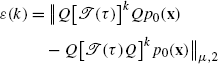
In order to remove the dependency on the initial distribution p ₀(x), we assume the worst case: the maximal possible value of ε(k) amongst all possible p ₀(x) is given by the operator-2-norm of the error matrix [Q[𝒯(τ)]^k Q−Q[𝒯(τ)Q]^k], where ∥A∥ _μ,2≡max_∥x∥=1∥Ax∥ _μ,2 [17], thus the Markov model error is defined as:

(3.42)

which measures the maximum possible difference between the true probability density at time kτ and the probability density predicted by the Markov model at the same time.

In order to quantify this error, we declare our explicit interest in the m slowest processes with eigenvalues 1=λ ₁>λ ₂≥λ ₃≥⋯≥λ _m . Generally, m≤n, i.e. we are interested in less processes than the number of n eigenvectors that a Markov model with n states has. We define the following two quantities:

• δ _i :=∥ψ _i (x)−Qψ _i (x)∥ _μ,2 is the eigenfunction approximation error, quantifying the error of approximating the true continuous eigenfunctions of the transfer operator, ψ _i (see Fig. 3.6 for illustration), for all i∈{1,…,m}. δ:=max _i δ _i is the largest approximation error amongst these first m eigenfunctions

  Fig. 3.6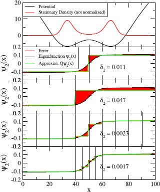

  

  Illustration of the eigenfunction approximation error δ ₂ on the slow transition in the diffusion in a double well (top, black line). The slowest eigenfunction is shown in the lower four panels (black), along with the step approximations (green) of the partitions (vertical black lines) at x=50; x=40; x=10,20,…,80,90; and x=40,45,50,55,60. The eigenfunction approximation error δ ₂ is shown as red area and its norm is printed

• $\eta(\tau):=\frac{\lambda_{m+1}(\tau)}{\lambda_{2}(\tau )}$ is the spectral error, the error due to neglecting the fast subspace of the transfer operator, which decays to 0 with increasing lag time: lim _τ→∞ η(τ)=0.

The general statement is that the Markov model error E(k) can be proven [36] to be bounded from above by the following expression:

$$ E(k)\le\min\bigl\{ 2,\bigl[m\delta+\eta(\tau)\bigr] \bigl[a(\delta)+b(\tau)\bigr] \bigr\} \lambda_{2}^{k} $$

(3.43)

with

$$\begin{aligned} a(\delta) = & \sqrt{m}(k-1)\delta, \end{aligned}$$

(3.44)

$$\begin{aligned} b(\tau) = & \frac{\eta(\tau)}{1-\eta(\tau)}\bigl(1-\eta(\tau)^{k-1}\bigr). \end{aligned}$$

(3.45)

This implies two observations:

• 1. For long times, the overall error decays to zero with $\lambda_{2}^{k}$, where 0<λ ₂<1, thus the stationary distribution (recovered as k→∞) is always correctly modeled, even if the kinetics are badly approximated.

• 2. The error during the kinetically interesting timescales consists of a product whose terms contain separately the discretization error and spectral error. Thus, the overall error can be diminished by choosing a discretization basis q ₁,…,q _n that approximates the slow eigenfunctions well, and using a large lag time τ. For a crisp partitioning this implies that the discretization has to be fine enough to trace the slow eigenfunctions well.

Depending on the ratio λ _m+1(τ)/λ ₂(τ), the decay of the spectral error η(τ) with τ might be slow. It is thus interesting to consider a special case of discretization that yields n=m and δ=0. This would be achieved by a Markov model that uses a fuzzy partition with membership functions q ₁,…,q _n derived from the first m eigenfunctions ψ ₁,…,ψ _m [24]. In this case, the space spanned by q ₁,…,q _n would equal the dominant eigenspace and hence the projection error would be δ=0. From a more practical point of view, this situation can be approached by using a Markov model with n>m states located such that they discretize the first m eigenfunctions with a vanishing discretization error, and then declaring that we are only interested in these m slowest relaxation processes. In this case we do not need to rely on the upper bound of the error from Eq. (3.43), but directly get the important result E(k)=0.

In other words, a Markov model can approximate the kinetics of slow processes arbitrarily well, provided the discretization can be made sufficiently fine or improved in a way that continues to minimize the eigenfunction approximation error. This observation can be rationalized by Eq. (3.19) which shows that the dynamics of the transfer operator can be exactly decomposed into a superposition of slow and fast processes.

An important consequence of the δ-dependence of the error is that the best partition is not necessarily metastable. Previous work [9, 9, 20, 32, 36, 42] has focused on the construction of partitions with high metastability (defined as the trace of the transition matrix T(τ)), e.g. the two-state partition shown in Fig. 3.6b). This approach was based on the idea that the discretized dynamics must be approximately Markovian if the system remained in each partition sufficiently long to approximately lose memory [9]. While it can be shown that if a system has m metastable sets with λ _m ≫λ _m+1, then the most metastable partition into n=m sets also minimizes the discretization error [36, 36], the expression for the discretization error given here has two further profound ramifications: First, even in the case where there exists a strong separation of timescales so the system has clearly m metastable sets, the discretization error can be reduced even further by splitting the metastable partition into a total of n>m sets which are not metastable. And second, even in the absence of a strong separation of timescales, the discretization error can be made arbitrarily small by making the partition finer, especially in transition regions, where the eigenfunctions change most rapidly (see Fig. 3.6b).

Figure 3.7 illustrates the Markov model discretization error on a two-dimensional three-well example where two slow processes are of interest. The left panels show a metastable partition with 3 sets. As seen in Fig. 3.7d, the discretization errors |ψ ₂−Qψ ₂|(x) and |ψ ₃−Qψ ₃|(x) are large near the transition regions, where the eigenfunctions ψ ₂(x) and ψ ₃(x) change rapidly, leading to a large discretization error. Using a random partition (Fig. 3.7, third column) makes the situation worse, but increasing the number of states reduces the discretization error (Fig. 3.7, fourth column), thereby increasing the quality of the Markov model. When states are chosen such as to well approximate the eigenfunctions, a very small error can be obtained with few sets (Fig. 3.7, second column).

Fig. 3.7

Illustration of the eigenfunction approximation errors δ ₂ and δ ₃ on the two slowest processes in a two-dimensional three-well diffusion model (see Supplementary Information for model details). The columns from left to right show different state space discretizations with white lines as state boundaries: (i) 3 states with maximum metastability, (ii) the metastable states were further subdivided manually into 13 states to better resolve the transition region, resulting in a partition where no individual state is metastable, (iii)/(iv) Voronoi partition using 25/100 randomly chosen centers, respectively. (a) Potential, (b) The exact eigenfunctions of the slow processes, ψ ₂(x) and ψ ₃(x), (c) The approximation of eigenfunctions with discrete states, Qψ ₂(x) and Qψ ₃(x), (d) Approximation errors |ψ ₂−Qψ ₂|(x) and |ψ ₃−Qψ ₃|(x). The error norms δ ₂ and δ ₃ are given

These results suggest that an adaptive discretization algorithm may be constructed which minimizes the E(k) error. Such an algorithm could iteratively modify the definitions of discretization sets as suggested previously [9], but instead of maximizing metastability it would minimize the E(k) error which can be evaluated by comparing eigenvector approximations on a coarse discretization compared to a reference evaluated on a finer discretization [36].

One of the most intriguing insights from both Eq. (3.19) and the results of the discretization error is that if, for a given system, only the slowest dynamical processes are of interest, it is sufficient to discretize the state space such that the first few eigenvectors are well represented (in terms of small approximation errors δ _i ). For example, if one is interested in processes on timescales t ^∗ or slower, then the number m of eigenfunctions that need to be resolved is equal to the number of implied timescales with t _i ≥t ^∗. Due to the perfect decoupling of processes for reversible dynamics in the eigenfunctions (see Eqs. (3.20)–(3.21)), no gap after these first m timescales of interest is needed. Note that the quality of the Markov model does not depend on the dimensionality of the simulated system, i.e. the number of atoms. Thus, if only the slowest process of the system is of interest (such as the folding process in a two-state folder), only a one-dimensional parameter, namely the level of the dominant eigenfunction, needs to be approximated with the clustering, even if the system is huge. This opens a way to discretize state spaces of very large molecular systems.

3.7 Approximation of Eigenvalues and Timescales by Markov Models

One of the most interesting kinetic properties of molecular systems are the intrinsic timescales of the system. They can be both experimentally accessed via relaxation or correlation functions that are measurable with various spectroscopic techniques [2, 5, 20, 28], but can also be directly calculated from the Markov model eigenvalues as implied timescales, Eq. (3.22). Thus, we investigate the question how well the dominant eigenvalues λ _i are approximated by the Markov model, which immediately results in estimates for how accurately a Markov model may reproduce the implied timescales of the original dynamics. Consider the first m eigenvalues of 𝒯(τ), 1=λ ₁(τ)>λ ₂(τ)≥⋯≥λ _m (τ), and let $1=\hat{\lambda}_{1}(\tau)>\hat{\lambda}_{2}(\tau)\ge \cdots\ge\hat{\lambda}_{m}(\tau)$ denote the associated eigenvalues of the Markov model T(τ). The rigorous mathematical estimate from [13] states that

$$ \max_{j=1,\ldots,m}\bigl\vert \lambda_{j}(\tau)-\hat{\lambda }_{j}(\tau)\bigr\vert \le(m-1)\lambda_{2}(\tau)\delta^{2}, $$

(3.46)

where δ is again the maximum discretization error of the first m eigenfunctions, showing that the eigenvalues are well reproduced when the discretization well traces these eigenfunctions. In particular if we are only interested in the eigenvalue of the slowest process, λ ₂(τ), which is often experimentally reported via the slowest relaxation time of the system, t ₂, the following estimate of the approximation error can be given:

$$ \frac{|\lambda_{2}(\tau)-\hat{\lambda}_{2}(\tau)|}{|\lambda _{2}(\tau)|}\le\delta_{2}^{2}. $$

(3.47)

As λ ₂(τ) corresponds to a slow process, we can make the restriction λ ₂(τ)>0. Moreover, the discretization error of Markov models based on full partitions of state space is such that the eigenvalues are always underestimated [13], thus $\lambda_{2}(\tau)-\hat{\lambda}_{2}(\tau)>0$. Using Eq. (3.22), we thus obtain the estimate for the discretization error of the largest implied timescale and the corresponding smallest implied rate, $k_{2}=t_{2}^{-1}$:

$$ \hat{t}_{2}^{-1}-t_{2}^{-1}= \hat{k}_{2}-k_{2}\le-\tau^{-1}\ln \bigl(1- \delta_{2}^{2}\bigr), $$

(3.48)

which implies that for either δ ₂→0₊ or τ→∞, the error in the largest implied timescale or smallest implied rate tends to zero. Moreover, since λ ₂(τ)→0 for τ→∞, this is also true for the other processes:

$$ \lim_{\tau\rightarrow\infty}\frac{|\lambda_{j}(\tau)-\hat {\lambda}_{j}(\tau)|}{|\lambda_{j}(\tau)|}=0, $$

(3.49)

and also

$$ \lim_{\delta\rightarrow0}\frac{|\lambda_{j}(\tau)-\hat{\lambda }_{j}(\tau)|}{|\lambda_{j}(\tau)|}=0, $$

(3.50)

which means that the error of the implied timescales also vanishes for either sufficiently long lag times τ or for sufficiently fine discretization. This fact has been empirically observed in many previous studies [2, 5, 9, 26, 32, 33, 42], but can now be understood in detail in terms of the discretization error. It is worth noting that observing convergence of the slowest implied timescales in τ is not a test of Markovianity. While Markovian dynamics implies constancy of implied timescales in τ [32, 42], the reverse is not true and would require the eigenvectors to be constant as well. However, observing the lag time-dependence of the implied timescales is a useful approach to choose a lag time τ at which T(τ) shall be calculated, but this model needs to be validated subsequently (see Chapter Estimation and Validation).

Figure 3.8 shows the slowest implied timescale t ₂ for the diffusion in a two-well potential (see Fig. 3.6) with discretizations shown in Fig. 3.6. The two-state partition at x=50 requires a lag time of ≈2000 steps in order to reach an error of <3 % with respect to the true implied timescale, which is somewhat slower than t ₂ itself. When the two-state partition is distorted by shifting the discretization border to x=40, this quality is not reached before the process itself has relaxed. Thus, in this system two states are not sufficient to build a Markov model that is at the same time precise and has a time resolution good enough to trace the decay of the slowest process. By using more states and particularly a finer discretization of the transition region, the same approximation quality is obtained with only τ≈1500 (blue) and τ≈500 steps (green).

Fig. 3.8

Convergence of the slowest implied timescale t ₂=−τ/lnλ ₂(τ) of the diffusion in a double-well potential depending on the MSM discretization. The metastable partition (black, solid) has greater error than non-metastable partitions (blue, green) with more states that better trace the change of the slow eigenfunction near the transition state

Figure 3.9 shows the two slowest implied timescales t ₂, t ₃ for the diffusion in a two-dimensional three-well potential with discretizations shown in Fig. 3.7a. The metastable 3-state partition requires a lag time of ≈1000 steps in order to reach an error of <3 % with respect to the true implied timescale, which is somewhat shorter than the slow but longer than the fast timescale, while refining the discretization near the transition states achieves the same precision with τ≈200 using only 12 states. A k-means clustering with k=25 is worse than the metastable partition, as some clusters cross over the transition region and fail to resolve the slow eigenfunctions. Increasing the number of clusters to k=100 improves the result significantly, but is still worse than the 12 states that have been manually chosen so as to well resolve the transition region. This suggests that excellent MSMs could be built with rather few states when an adaptive algorithm that more finely partitions the transition region is employed.

Fig. 3.9

Implied timescales for the two slowest processes in the two-dimensional three-well diffusion model (see Fig. 3.7a for potential and Supplementary Information for details). The colors black, red, yellow, green correspond to the four choices of discrete states shown in columns 1 to 4 of Fig. 3.7. A fine discretization of the transition region clearly gives the best approximation to the timescales at small lag times

Note that the estimate (3.46) bounds the maximal eigenvalue error for the dominant eigenvalues by the maximal projection error of the dominant eigenfunction. In [34], it is also shown that if u is a selected, maybe non-dominant eigenfunctions for an eigenvalue λ(τ) and δ=∥u−Qu∥ is its discretization error, the associated MSM will inherit an eigenvalue $\hat{\lambda}(\tau)$ with

$$ \bigl\vert \lambda(\tau)-\hat{\lambda(\tau)}\bigr\vert \le2\lambda_2(\tau)\delta $$

(3.51)

if δ=∥u−Qu∥≤3/4. That is, it is also possible to approximate selected timescales well by choosing the discretization such that it traces the associated eigenfunctions well without having to take all slower eigenfunctions into account [34].

3.8 An Alternative Set-Oriented Projection

In the last sections, we have derived an interpretation of Markov models as projections of the transfer operator 𝒯(τ) and connected their discretization error in terms of density propagation and in terms of eigenvalue and timescale approximation to projection errors. Estimates for these quality measures show that the discretization basis should be chosen such that it traces the slow eigenfunctions well. For a crisp partitioning this means that the eigenfunctions should be well approximated by step-functions induced by the sets S ₁,…,S _n . On the other hand, the results are not restricted to projections onto step-functions. Theoretically, one could choose an arbitrary discretization basis q ₁,…,q _n for constructing the Markov model, see [40], and the corresponding MSM matrix would formally be given by T(τ)=T(τ)M ⁻¹ (3.35). In praxis, the basis q ₁,…,q _n has be chosen such that it leads to interpretable matrices T(τ) and M in terms of transition probabilities between sets. Otherwise, one will not be able compute estimates for these matrices and thus for the resulting Markov model. For a crisp partitioning S ₁,…,S _n and the associated characteristic functions χ ₁,…,χ _n we have this property

$$T_{ij}(\tau) = \mathbb{P}\bigl[\mathbf{x}(t+\tau)\in S_{j} \bigm|\mathbf {x}(t)\in S_{i}\bigr], \quad M=Id. $$

The drawback of this method is that coarse partitionings always lead to coarse step-functions that might not approximate the eigenfunctions well. Therefore, a refinement might be necessary in regions where the slow eigenfunctions are varying strongly.

In this section, we will show how to derive another set-oriented discretization basis where a rather coarse partitioning does not lead to a coarse discretization basis. The main idea goes back to [32, 37, 40]: simply decrease the size of the sets S ₁,…,S _n on which the constancy of the discretization basis in enforced. Of course, the resulting sets do not cover the whole state space and hence do not form a crisp partitioning anymore. We will call such sets core sets in the following and denote them by C ₁,…,C _n in order to distinguish from a crisp partitioning S ₁,…,S _n .

The two questions that we have to answer are (a) how these core sets induce a discretization basis that approximates the slow eigenfunctions well, and (b) how to interpret the transition probabilities between the core sets to calculate the transition matrices T(τ) and M with respect to this basis. The idea is to attach a fuzzy partitioning to the core sets that is connected to the dynamics of the process itself. For every core set C _i we define the so called committor function

$$ q_i(x) = \mathbb{P}\bigl[x(\sigma) \in C_i \bigm| x(0) = x\bigr], $$

(3.52)

where σ is the first time one of the core sets is entered by the process.

That is, q _i (x) is the probability that the process will hit the set C _i next rather than the other core sets when being started in point x. From the definition it follows that [27, 40]

$$\begin{aligned} &q_i(x) = 1 \quad\text{for all } x\in C_i, \\ &q_i(x) = 0 \quad\text{for all } x\in C_j, j\neq i,\\ &\sum_i q_i(x) = 1 \quad\text{for all } x. \end{aligned}$$

The advantage of taking committor functions as discretization basis is that the core sets, on which the committor functions equal to characteristic functions, do not have to cover the whole state space. It is allowed to have a region C=Ω∖⋃ _j C _j that is not partitioned and where the values of the committor functions can continuously vary between 0 and 1. This means that the part of state space can be shrinked, where the slow eigenfunctions need to be similar to step-functions. Moreover, it has been shown in [34] that the approximation of the slow eigenfunctions by the committors inside of the fuzzy region C is accurate if the region C is left by the process quickly enough. Being more precise, this approximation error is dominated by the ratio of the expected time the process needs to leave the region C and the implied timescale that is associated with the target eigenfunction. We will see that it is computationally very suitable that this is the main constraint on C.

Beside the good approximation of the slow eigenfunctions, the committor discretization has another advantage. We can calculate the Markov model from transition probabilities between the core sets without having to compute the committor functions explicitly. It is shown in [32, 37, 40] that for the committor basis we can interpret the matrices T(τ) and M as follows:

Define x ⁺(t) as the index of the core set that is hit next after time t, and x ⁻(t) as the index of the core set that the process has visited last before time t, then

$$M_{ij} = \mathbb{P}\bigl[x^+(t) = j \bigm| x^-(t) = i\bigr], $$

and

$$T_{ij}(\tau) = \mathbb{P}\bigl[x^+(t+\tau) = j \bigm| x^-(t) = i \bigr]. $$

Note that this can be interpreted in terms of a transition behavior. If we interpret T _ij (τ) as the probability that a transition occurs from index i at time t to index j at time t+τ, then we say a transition has occurred if the process was in core set i at time t or at least came last from this set and after a time-step τ it was in core set j or at least went next to this set afterwards. Figure 3.10 illustrates this interpretation. As mentioned above, these transition probabilities can be directly estimated from realizations without having to compute the committor functions.

Fig. 3.10

Counting a transition in the sense of T ₁₂(τ) for a crisp partitioning (left hand side) and for core sets (right hand side) that do not cover the whole state space

The effect on the approximation of the slowest eigenfunction can be seen in Fig. 3.11.

Fig. 3.11

The benefit of removing a part of state space that is typically left quickly by the process. On the left hand side: step-function approximation of the first non-trivial eigenfunction. Right hand side: committor approximation of the same eigenfunction

Computationally, there is an important insight. Assume a crisp partitioning of state space into n sets S ₁,…,S _n is given. Now, a committor discretization would allow to avoid a part of state space from being discretized, as long as the process leaves this part typically much faster than the interesting timescales. On the one hand, these parts of state space exactly correspond to regions where the slow eigenfunctions are varying strongly. So starting from the crisp partitioning we can benefit most by simply ignoring this part of state space and treating the remaining sets as core sets. On the other hand, removing such part of state space, where the process does not spend a lot of time in, does not effect the computational effort in order to generate transitions with respect to the crisp partitioning or the resulting core sets as in Fig. 3.10. Summarizing, one can always enhance a model based on a crisp partitioning by simply declaring a part of state space as not belonging to the discretization anymore, as long as this part of state space is usually left quickly by the process, and computationally one can get this enhancement for free.

Let us illustrate this feature by an example. We consider again a diffusion in the potential that is illustrated in Fig. 3.12. Now, Fig. 3.13 shows an optimal crisp partitioning into 9 sets, where every well of the potential falls into another partitioning set. Moreover, it shows the core set discretization where only a part of the transition region between the wells was excluded from the crisp discretization.

Fig. 3.12

Example: diffusion in this multi-well potential

Fig. 3.13

A metastable crisp partitioning into 9 sets (left), and the derived core set discretization by removing the transition region between the wells (right)

The approximation by a step-function is too coarse while removing the transition region and shrinking the size of the sets leads to a smoother and better interpolation of the eigenfunction. As we discussed in the previous sections, this has a direct impact on the approximation quality of the associated Markov model. For example, the following table shows the implied timescales t _i of the original Markov process and the approximations by the crisp partitioning and the enhanced core set MSM.

	t 2	t 3	t 4	t 5
original	17.5267	3.1701	0.9804	0.4524
core sets	17.3298	3.1332	0.9690	0.4430
crisp partition	16.5478	2.9073	0.8941	0.4006

As expected, the approximation quality in terms of timescale approximation could be increased by simply removing a small part of state space from the discretization. The same enhancement is achieved with respect to the density propagation error E(k) (3.42). Figure 3.14 compares the resulting error for the crisp partitioning (black) and the core set discretization (blue) and increasing k.

Fig. 3.14

Density propagation error E(k) over k. Black: crisp partitioning. Blue: core sets

References

Andersen HC (1980) Molecular dynamics simulations at constant pressure and/or temperature. J Chem Phys 72(4):2384–2393. doi:10.1063/1.439486
Bieri O, Wirz J, Hellrung B, Schutkowski M, Drewello M, Kiefhaber T (1999) The speed limit for protein folding measured by triplet-triplet energy transfer. Proc Natl Acad Sci USA 96(17):9597–9601. http://www.pnas.org/content/96/17/9597.abstract
Bowman GR, Beauchamp KA, Boxer G, Pande VS (2009) Progress and challenges in the automated construction of Markov state models for full protein systems. J Chem Phys 131(12):124,101+. doi:10.1063/1.3216567
Buchete NV, Hummer G (2008) Coarse Master Equations for Peptide Folding Dynamics. J Phys Chem B 112:6057–6069
Chan CK, Hu Y, Takahashi S, Rousseau DL, Eaton WA, Hofrichter J (1997) Submillisecond protein folding kinetics studied by ultrarapid mixing. Proc Natl Acad Sci USA 94(5):1779–1784. http://www.pnas.org/content/94/5/1779.abstract
Chodera JD, Dill KA, Singhal N, Pande VS, Swope WC, Pitera JW (2007) Automatic discovery of metastable states for the construction of Markov models of macromolecular conformational dynamics. J Chem Phys 126:155,101
Chodera JD, Noé F (2010) Probability distributions of molecular observables computed from Markov models, II: uncertainties in observables and their time-evolution. J Chem Phys 133:105,102
Chodera JD, Swope WC, Noé F, Prinz JH, Pande VS (2010) Dynamical reweighting: improved estimates of dynamical properties from simulations at multiple temperatures. J Phys Chem. doi:10.1063/1.3592152
Chodera JD, Swope WC, Pitera JW, Dill KA (2006) Long-time protein folding dynamics from short-time molecular dynamics simulations. Multiscale Model Simul 5:1214–1226
Cooke B, Schmidler SC (2008) Preserving the Boltzmann ensemble in replica-exchange molecular dynamics. J Chem Phys 129:164,112
Deuflhard P, Huisinga W, Fischer A, Schütte C (2000) Identification of almost invariant aggregates in reversible nearly uncoupled Markov chains. Linear Algebra Appl 315:39–59
Deuflhard P, Weber M (2005) Robust Perron cluster analysis in conformation dynamics. Linear Algebra Appl 398:161–184
Djurdjevac N, Sarich M, Schütte C (2012) Estimating the eigenvalue error of Markov state models. Multiscale Model Simul 10(1):61–81
Duane S (1987) Hybrid Monte Carlo. Phys Lett B 195(2):216–222. doi:10.1016/0370-2693(87)91197-X
Ermak DL (1975) A computer simulation of charged particles in solution, I: technique and equilibrium properties. J Chem Phys 62(10):4189–4196
Ermak DL, Yeh Y (1974) Equilibrium electrostatic effects on the behavior of polyions in solution: polyion-mobile ion interaction. Chem Phys Lett 24(2):243–248
Golub GH, van Loan CF (1996) Matrix computations, 3rd edn. John Hopkins University Press, Baltimore
Herau R, Hitrik M, Sjoestrand J (2010) Tunnel effect and symmetries for Kramers Fokker-Planck type operators. arXiv:1007.0838v1
Huisinga W (2001) Metastability of Markovian systems: a transfer operator based approach in application to molecular dynamics. PhD thesis, Fachbereich Mathematik und Informatik, FU Berlin
Huisinga W, Meyn S, Schütte C (2004) Phase transitions and metastability for Markovian and molecular systems. Ann Appl Probab 14:419–458
Jäger M, Nguyen H, Crane JC, Kelly JW, Gruebele M (2001) The folding mechanism of a beta-sheet: the WW domain. J Mol Biol 311(2):373–393. doi:10.1006/jmbi.2001.4873
van Kampen NG (2006) Stochastic processes in physics and chemistry, 4th edn. Elsevier, Amsterdam
Keller B, Hünenberger P, van Gunsteren W (2010) An analysis of the validity of Markov state models for emulating the dynamics of classical molecular systems and ensembles. J Chem Theor Comput. doi:10.1021/ct200069c
Kube S, Weber M (2007) A coarse graining method for the identification of transition rates between molecular conformations. J Chem Phys 126:024,103–024,113
Meerbach E, Schütte C, Horenko I, Schmidt B (2007) Metastable conformational structure and dynamics: peptides between gas phase and aqueous solution. Series in chemical physics, vol 87. Springer, Berlin, pp 796–806
Metzner P, Horenko I, Schütte C (2007) Generator estimation of Markov jump processes based on incomplete observations nonequidistant in time. Phys Rev E 76(6):066,702+. doi:10.1103/PhysRevE.76.066702
Metzner P, Schütte C, Vanden-Eijnden E (2009) Transition path theory for Markov jump processes. Multiscale Model Simul 7(3):1192–1219
Neuweiler H, Doose S, Sauer M (2005) A microscopic view of miniprotein folding: enhanced folding efficiency through formation of an intermediate. Proc Natl Acad Sci USA 102(46):16,650–16,655. doi:10.1073/pnas.0507351102
Noé F, Horenko I, Schütte C, Smith JC (2007) Hierarchical analysis of conformational dynamics in biomolecules: transition networks of metastable states. J Chem Phys 126:155,102
Noé F, Schütte C, Vanden-Eijnden E, Reich L, Weikl TR (2009) Constructing the full ensemble of folding pathways from short off-equilibrium simulations. Proc Natl Acad Sci USA 106:19,011–19,016
Prinz JH et al. (2011) Markov models of molecular kinetics: generation and validation. J Chem Phys 134:174,105
Sarich M (2011) Projected transfer operators. PhD thesis, Freie Universität Berlin
Sarich M, Noé F, Schütte C (2010) On the approximation error of Markov state models. Multiscale Model Simul 8:1154–1177
Sarich M, Schütte C (2012) Approximating selected non-dominant timescales by Markov state models. Comm Math Sci (in press)
Schütte C (1998) Conformational dynamics: modelling, theory, algorithm, and applications to biomolecules. Habilitation thesis, Fachbereich Mathematik und Informatik, FU Berlin
Schütte C, Huisinga W (2003) Biomolecular conformations can be identified as metastable sets of molecular dynamics. In: Handbook of numerical analysis. Elsevier, Amsterdam, pp 699–744
Schütte C, Sarich M (2013) Metastability and Markov state models in molecular dynamics: modeling, analysis, algorithmic approaches. Courant lecture notes, vol 24. American Mathematical Society, Providence
Schütte C, Fischer A, Huisinga W, Deuflhard P (1999) A direct approach to conformational dynamics based on hybrid Monte Carlo. J Comput Phys 151:146–168
Schütte C, Noé F, Meerbach E, Metzner P, Hartmann C (2009) Conformation dynamics. In: Jeltsch RGW (ed) Proceedings of the international congress on industrial and applied mathematics (ICIAM). EMS Publishing House, New York, pp 297–336
Schütte C, Noé F, Lu J, Sarich M, Vanden-Eijnden E (2011) Markov state models based on milestoning. J Chem Phys 134(19)
Sriraman S, Kevrekidis IG, Hummer G (2005) Coarse master equation from Bayesian analysis of replica molecular dynamics simulations. J Phys Chem B 109:6479–6484
Swope WC, Andersen HC, Berens PH, Wilson KR (1982) A computer simulation method for the calculation of equilibrium constants for the formation of physical clusters of molecules: application to small water clusters. J Chem Phys 76(1):637–649
Swope WC, Pitera JW, Suits F (2004) Describing protein folding kinetics by molecular dynamics simulations, 1: theory. J Phys Chem B 108:6571–6581
Swope WC, Pitera JW, Suits F, Pitman M, Eleftheriou M (2004) Describing protein folding kinetics by molecular dynamics simulations, 2: example applications to alanine dipeptide and beta-hairpin peptide. J Phys Chem B 108:6582–6594
Voronoi MG (1908) Nouvelles applications des parametres continus a la theorie des formes quadratiques. J Reine Angew Math 134:198–287
Weber M (2006) Meshless methods in conformation dynamics. PhD thesis, Freie Universität Berlin
Weber M (2010) A subspace approach to molecular Markov state models via an infinitesimal generator. ZIB report 09-27-rev
Weber M (2011) A subspace approach to molecular Markov state models via a new infinitesimal generator. Habilitation thesis, Fachbereich Mathematik und Informatik, Freie Universität Berlin
Author information
Authors and Affiliations
Corresponding author
Editor information
Editors and Affiliations
Rights and permissions
Copyright information
© 2014 Springer Science+Business Media Dordrecht
About this chapter
Cite this chapter
Sarich, M., Prinz, JH., Schütte, C. (2014). Markov Model Theory. In: Bowman, G., Pande, V., Noé, F. (eds) An Introduction to Markov State Models and Their Application to Long Timescale Molecular Simulation. Advances in Experimental Medicine and Biology, vol 797. Springer, Dordrecht. https://doi.org/10.1007/978-94-007-7606-7_3
Download citation
DOI: https://doi.org/10.1007/978-94-007-7606-7_3
Publisher Name: Springer, Dordrecht
Print ISBN: 978-94-007-7605-0
Online ISBN: 978-94-007-7606-7
eBook Packages: Biomedical and Life SciencesBiomedical and Life Sciences (R0)