Logic Programming and Prolog

Abstract

Prolog  is logic programming languages for AI, based on predicate logic. This chapter discusses the structure, syntax, and semantics of Prolog language, provides comparison with procedural language like C, interpretation of predicate logic and that of Prolog, both formally as well through worked out examples, and explain how the recursion is definition as well solution of a problem, and explains with simple examples as how the control sequencing takes place in Prolog. Use of two open source compilers of prolog using simple worked out examples is demonstrated. Each concept of Prolog and logic programming is explained with the help of worked out examples. At the end, a brief summary gives glimpse of the chapter, followed with number of exercises to strengthen the learning.

5.1 Introduction

This chapter presents the basic concepts of logic programming, and Prolog language. Prolog is a logic programming language, implemented in two parts:

• 1. Logic, which describes the problem, and

• 2. Control, provides the solution method.

This is in contrast to procedural programming languages, where description and solution go together, and are hardly distinguishable. This, feature of prolog helps in separate developments for each part, one by the programmer and other by implementer.

PROLOG is a simple, yet powerful programming language, based on the principles of first-order predicate logic. The name of the language is an acronym for the French ‘PROgrammation en LOGique’(programming in logic). PROLOG was designed by A. Colmerauer and P. Roussel at the University of Marseille (Canada), around 1970. The PROLOG has remained connected with a new programming style, known as logic programming. Prolog is useful in problem areas, such as artificial intelligence, natural language processing, databases, etc., but pretty useless in others, such as graphics or numerical computations. The main applications of the language can be found in the area of Artificial Intelligence; but PROLOG is being used in other areas in which symbol manipulation is of prime importance. Following are the application areas.

• Computer algebra.

• Design of parallel computer architectures.

• Database systems.

• Natural-language processing.

• Compiler construction.

• Design of expert systems.

The popular compilers of prolog are swi-prolog and gnu prolog; both are available in open source, and runs on Windows and Linux platforms.

Learning Outcomes of this Chapter:

• 1. Prolog versus procedure-oriented languages. [Assessment]

• 2. Working with Prolog, using gprolog and swi-prolog compilers. [Usage]

• 3. Writing small prolog programs and running. [Usage]

• 4. Translating predicate logic into Prolog. [Usage]

• 5. Prolog Syntax and semantics. [Familiarity]

• 6. Forward-chaining versus back-ward chaining. [Assessment]

• 7. Using backward-chaining for reasoning and inference in Prolog. [Assessment]

5.2 Logic Programming

 

In conventional languages, like, C, C$++$, and Java, a program is a description of sequence of instructions to be executed one-by-one by a target machine to solve the given problem. The description of the problem is implicitly incorporated in this instruction sequence, where usually it is not possible to clearly distinguish between the description (i.e., logic) of the problem, and the method (i.e., control) used for its solution.

In logic programming language, like Prolog, the description of the problem and the method for its solution are explicitly separated from each other. Hence, in an algorithm of a Prolog program, these two parts are distinctly visible, and can be expressed by [6]:

(5.1)

In the above equation, term ‘logic’ represents the descriptive part of an algorithm, and ‘control’ represents the solution part, which takes the description as the point of departure. In other words, the logic component defines what the algorithm is supposed to do, and the control component indicates how it should be done.

For solution through logic program, a problem is always described in terms of relevant objects and relations between them. These relations are represented in a clausal form of logic—a restricted form of first-order predicate logic. The logic component for a problem is called a logic program, while the control component comprises method for logical deduction (reasoning) for deriving new facts from the logic program. This results to solving a problem through deduction. The deduction method is designed as a general program, such that it is capable of dealing with any logic program that follows the clausal form of syntax.

There are number of advantages of splitting of an algorithm into a logic component and a control component:

• We can develop these two components of the program independent of each other. For example, when writing the description of the problem as logic, we do not have to be familiar with how the control component operates for that problem; thus knowledge of the declarative reading of the problem specification suffices.

• A logic component may be developed using a method of stepwise refinement; we have only to watch over the correctness of the specification.

• Changes to the control component affect (under certain conditions) only the efficiency of the algorithm; they do not influence the solutions produced.

The implementation of Logic programming is explained in Fig. 5.1.

Fig. 5.1

Logic programming

When all facts and rules have been identified, then a specific problem may be looked upon as a query concerning the objects and their interrelationships. In summary, to provide specification of a logic program amounts to following jobs:

• specify the facts about the objects and relations between them for the problem being solved;

• specify the rules about the objects and their interrelationships;

• specify the queries to be posed concerning the objects and relations.

An algorithm for logic program can be shown to be decomposed into the components shown in Fig. 5.2.

Fig. 5.2

Components of logic program

5.3 Interpretation of Horn Clauses in Rule-Chaining

 

Horn clause is restricted form of a predicate logic sentence. A typical representation of a problem in Horn clause form is:

• 1. a set of clauses defining a problem domain and,

• 2. a theorem consisting of: (a) hypotheses represented by assertions $A_1 \leftarrow , \dots , A_n \leftarrow$ and (b) a conclusion in negated form and represented by a denial $\leftarrow B_1, \dots , B_m$.

The reasoning process can be carried out as back-ward reasoning, or forward reasoning. In backward-chaining, reasoning is performed backwards from the conclusion, which repeatedly reduces the goals to subgoals until ultimately all the subgoals are solved directly in the form of original assertions.

In the case of problem-solving using forward-chaining approach, we reason forwards from the hypotheses, and repeatedly derive new assertions from old ones until eventually the original goal is solved directly by derived assertions [6].

For our reasoning using forward and backward chaining, we consider the family-tree of Mauryan Dynasty (India) as shown in Fig. 5.3 [5].

Fig. 5.3

Mauryan dynasty family-tree

The problem of showing that chandragupta is a grandparent of ashoka can be solved either backward-chaining or forward-chaining. In forward-chaining, we start with the following assertions:

father(bindusara, asoka) $\leftarrow$

father(chandragupta, bindusara) $\leftarrow$

Also, we shall use the clause $parent(x, y) \leftarrow father(x, y)$ to derive new assertions,

$parent(chandragupta, bindusara)\leftarrow$

$parent(bindusara, ashoka)\leftarrow$

Continuing forward-chaining we derive, from the definition of grandparent, the new assertion,

$grandparent(chandragupta, ashoka)\leftarrow$

which matches the original goal.

Reasoning using backward-chaining, we start with the original goal, which shows that chandragupta is a grandparent of ashoka,

$\leftarrow grandparent(chandragupta, ashoka)$

and use the definition of grandparent to derive two new subgoals,

$\leftarrow parent(chandragupta, z), parent(z, ashoka)$,

by denying that any z is both a child of chandragupta and a parent of ashoka. Continuing backward-chaining and considering both subgoals (either one at a time or both simultaneously), we use the clause,

$$\begin{aligned} parent(x, y) \leftarrow father(x, y) \end{aligned}$$

to replace the subproblem parent(chandragupta, z) by father(chandragupta, z) and the subproblem parent(z, ashoka) by father (z, ashoka). The symbol “$\leftarrow$” is read as “if”. The newly derived subproblems are solved compatibly by assertions which determine “bindusara” as the desired value of z.

In both the backward-chaining and forward-chaining solutions of the grandparent problem, we have mentioned the derivation of only those clauses which directly contribute to the ultimate solution. In addition to the derivation of relevant clauses, it is often unavoidable, during the course of searching for a solution, to derive assertions or subgoals which do not contribute to the solution. For example, in the forward-chaining search for a solution to the grandparent problem, it is possible to derive the irrelevant assertions as,

$parent(durdhara, bindusara)\leftarrow$

$male(chandragupta)\leftarrow$

Also, in backward-chaining search it is possible to replace the subproblem,

parent(chandragupta, z)

by the unsolvable and irrelevant subproblem,

mother(chandragupta, z).

There are proof procedures which understand logic in backward-chaining, e.g., model elimination, resolution, and interconnectivity graphs. These proof procedures operate with the clausal form of predicate logic and deal with both Horn clauses and non-Horn clauses. Among clausal proof procedures, the connection graph procedure is able to mix backward and forward reasoning.

The terminology we used here—the backward-chaining, is also called “top-down”. Given a grammar formulated in clausal form, top-down parsing algorithm generates a sentence to its original form, i.e., the assertions. The forward-chaining is also called “bottom-up”, where we start from the assertions and try to reach to the goals.

5.4 Logic Versus Control

Different control strategies for the same logical representation generate different behaviors. Also, the information about a problem-domain can be represented using logic in different ways. Alternative representations can have a more significant impact on the efficiency of an algorithm compared to alternative control strategies for the same representation.

Consider the problem of sorting a list x and obtaining the list y. In our representation, we can have a definition with an assertion consisting of two arguments: “y is permutation of x”, and “y is ordered”, i.e.,

sorting x gives $y \leftarrow y$ is a permutation of x, y is ordered.

Here “$\leftarrow$” is read as ‘if’ and ‘,’ is logical AND operator. The first argument generates permutations of x and then it is tested whether they are ordered. Executing procedure calls as coroutines, the procedure generates permutations, one element at a time. Whenever a new element is generated, the generation of other elements is suspended while it is determined whether the new element preserves the orderedness of the existing partial permutation.

A program consists of a logic component and a control component. The logic component defines the part of the algorithm that is problem specific, which not only determines the meaning of algorithm but also decides the way the algorithm behaves. For systematic development of well-structured programs using successive refinements, the logic component needs to be defined before the control component. Due to these two components of a logic program, the efficiency of an algorithm can be improved through two different approaches: 1. by improving the efficiency of logic component, 2. through the control component. Note, that both improvements are additive, and not as alternative choices.

In a logic programs, the specification of control component is subordinate to logic component. The control part can be explicitly specified by the programmer through a separate control specification language, or the system itself can determine the control. When logic is used like in relational calculus to specify queries (i.e., higher level of language) to knowledge base, the control component is entirely determined by the system. Hence, for higher level of programming language, like queries, lesser effort is required for programming the control part, because in that case the system assumes more responsibility about efficiency, as well as to exercise control over the use of given information.

Usually, a separate control-specifying language is preferred by advanced programmers to exercise the control with higher precision. A higher system efficiency is possible if programmer can communicate to system a more precise information to have finer control. Such information may be a relation, for example, F(x, y), where y can also be a function of x. This function could be used by a backtracking interpreter to avoid looking for another solution to the first goal in the goal statement. This can be expressed, for example by,

$\leftarrow F(A,y), G(y)$,

when the second goal fails. Other example of such information can be that one procedure,

$S \leftarrow T$

may be more likely to solve problem S than another procedure,

$S \leftarrow R$.

This kind of information of cause-effect relation is common in fault diagnosis where, on the basis of past experience, it might be possible to estimate that symptom S is more likely have been caused by T rather than by R.

In the above examples, the control information is problem-specific. However, if the control information is correct, and the interpreter is correctly implemented, then the control information should not affect the meaning of the algorithm, which is decided by the corresponding logic component of the program.

5.4.1 Data Structures

 

In a well-structured program it is desirable to keep data structures separate from procedure that interact with the data structure. Such separation means data structures can be manipulated without altering the procedure. Usually, there is need of alteration of data structures—some times due to the need of change of requirements and other times with an objective to to improve the algorithm by replacing data structure by a more efficient one. In large and complex programs, often the information demand made on the data structures are only determinable in the final stages of the program design. If data structures are separated from the procedures, the higher level procedures can be written before the data structures are finalized, and these procedures can be altered conveniently later any time without effecting the data structure [6].

In Prolog, the data structures of a program are already included in the logic component of the program. Consider, for example, the data structure “Lists”, which can be represented by following terms:

• nil; empty list,

• cons(x, y); list with first element x, and y is another list.

Hence, the following example names a three-element list consisting of individuals as 2, 1, 3 in that order.

cons(2, cons(1, cons(3, nil)))

Example 5.1

A logic program for quick-sort.

In quick-sort, the predicates empty, first, rest, partitioning, and appending, can be defined independently from the definition of sorting (see Eqs. 5.2 and 5.3). For this definition we assume that, partitioning of a list $x_2$ by element $x_1$ gives a list u comprising the elements of $x_2$ that are less or equal to $x_1$, and a list v of elements of $x_2$ that are greater than $x_1$.

$$\begin{aligned} sorting~x~gives~y~\leftarrow x~is~empty,~y~is~empty \end{aligned}$$

(5.2)

$$\begin{aligned} sorting~x~gives~y \leftarrow&first~element~of~x~is~x_1,~rest~is~x_2, \nonumber \\&partitioning~x_2~by~x_1~gives~u~and~v,\nonumber \\&sorting~u~gives~u^\prime ,\nonumber \\&sorting~v~gives~v^\prime ,\nonumber \\&appending~w~to~u^\prime gives~y,\nonumber \\&first~element~of~w~is~x_1,\nonumber \\&rest~of~w~is~v^\prime . \end{aligned}$$

(5.3)

The data-structure-free definition of quicksort interacts with the data structure of lists through the following definitions:

nil is empty $\leftarrow$

first element of $cons(x, y) is x \leftarrow$

rest of $cons(x, y) is y \leftarrow$

If the predicates: empty, first, rest, are dropped from the definition of quick-sort, and instead the preliminary forward-chaining/forward-chaining deduction is used, then the original data-structure-free definition of quick-sort can be replaced by a definition that mixes the data structures with the procedures,

$$\begin{aligned} sorting~nil~gives~nil\leftarrow \end{aligned}$$

$$\begin{aligned} sorting~cons(x_1, x_2)~gives~y \leftarrow&partitioning~x_2~by~x_1~gives~u, v,\\&sorting~u~gives~u^\prime ,\\&sorting~v~gives~v^\prime ,\\&appending~list~cons(x_1, v^\prime )~to~ u^\prime gives~y.~~~~ \end{aligned}$$

   $\square$

There is another advantage of data-structure-independent definition: with well-chosen interface procedure names, data-structure-independent programs are virtually self-documenting. In conventional programs that mix procedures and data structures, the programmer needs to provide separate documentation for data structures.

On the other hand, in-spite of the arguments in support for separating procedures and data structures, the programmers usually mix them together for the sake of run-time efficiency.

5.4.2 Procedure-Call Execution

 

In a simplest backward reasoning based execution, the procedure calls are executed one at a time, in the order they have been written. Typically, an algorithm can be made to run faster by executing the same procedure calls in the form of coroutines or as communicating parallel-processes. Consider an algorithm $A_1$,

$$\begin{aligned} A_1 = L + C_1 \end{aligned}$$

(5.4)

where logic component is L and control component is $C_1$. Assume that from $A_1$ we have obtained a new algorithm $A_2$, having logic component L and control component $C_2$,

$$\begin{aligned} A_2 = L + C_2 \end{aligned}$$

(5.5)

where we replaced control strategy $C_1$ by new control strategy $C_2$, and the logic L of the algorithm remains unchanged. For example, executing procedure calls in sequence, the procedure,

$$\begin{aligned} sorting~x~gives~y \leftarrow y~is~a~permutation~of~x,~y~is~ordered, \end{aligned}$$

(5.6)

first generates permutations of x and then tests whether they are ordered. By executing procedure calls as coroutines, the procedure generates permutations, one element at a time. Whenever a new element is generated, the generation of other elements is suspended while it is determined whether the new element preserves the orderedness of the existing partial permutation.

In the Similar way to procedure (5.6), procedure calls in the body of quick-sort can be executed (either as coroutines or as parallel/sequential processes). When they are executed in parallel, partitioning the rest of x can be initiated as soon as the first element of the rest are generated (see procedure (5.3) on p. 118). Note that the sorting for u and v can take place in parallel, the moment first elements of u and v are generated. And, the appending of lists can start soon after the first elements of $u^\prime$, and the sorted output of u, are made available.

The high level language SIMULA provides the facility of writing both the usual sequential algorithms, as well as algorithms with coroutines. Here, the programmer can provide the controls about: When the coroutines should be suspended and resumed? However, in this language, the logic and control are inextricably intertwined in the program text, like in other procedure oriented languages. Hence, the control of an algorithm cannot be modified without rewriting the entire program.

In one way, the concept of separating logic and controls is like separating data structures and procedures. When a procedure is kept separate from a data structure, we are able to distinguish clearly as what functions are fulfilled by which data structures. On the other hand, when logic is separated from control, it becomes possible to distinguish, what the program (i.e., logic) does, and how it does it (i.e., controlling takes place). In both conditions it becomes obvious as what the program does, and hence it can be more easily determined whether it correctly does the job it was intended for.

5.4.3 Backward Versus Forward Reasoning

 

Recursive definitions are common in mathematics, where they are more likely to be understood as forward-chaining rather than backward-chaining. Consider, for example, the definition of factorial, given below.

$$\begin{aligned} factorial~of~0~is~1 \leftarrow \end{aligned}$$

(5.7)

$$\begin{aligned} factorial~of~x~is~u \leftarrow&y~plus~1~is~x,\nonumber \\&factorial~of~y~is~v,\nonumber \\&x~times~v~is~u. \end{aligned}$$

(5.8)

The mathematician is likely to understand such a definition forward-chaining, generating the sequence of assertions as follows:

$$\begin{aligned} factorial~of~0~is~1 \leftarrow \\ factorial~of~1~is~1 \leftarrow \\ factorial~of~2~is~2 \leftarrow \\ factorial~of~3~is~6 \leftarrow \\ and~so~on. \end{aligned}$$

Conventional programming language implementations understand recursions as backward-chaining. Programmers, accordingly, tend to identify recursive definitions with backward-chaining execution. However, there is one exception, and that is Fibonacci series, which is efficient when interpreted as forward reasoning. It is left as an exercises for the students to verify the same.

5.4.4 Path Finding Algorithm

Consider an algorithm A, with $C_1, C_2$ control components, and $L_1, L_2$ as logic components, which can often be analyzed in different ways [6].

$$\begin{aligned} A = L_1 + C_1 = L_2 + C_2. \end{aligned}$$

(5.9)

Some of the behavior determined by $C_1$ in one analysis might be determined by the logic component $L_2$ in another analysis. This has significance for understanding the relationship between programming style and execution facilities. In the short term sophisticated behavior can be obtained by employing simple execution strategies and by writing complicated programs. In the longer term the same behavior may be obtained from simpler programs by using more sophisticated execution strategies.

A path-finding problem illustrates a situation in which the same algorithm can be analyzed in different ways. Consider the problem of finding a path from vertex a to vertex z in the directed graph shown in Fig. 5.4.

Fig. 5.4

Directed graph path finding

In one analysis, we can employ a predicate go(x) which states that it is possible to go to x. The problem of going from a to z is then represented by two clauses. One asserts that it is possible to go to a. The other denies that it is possible to go to z. The arc directed from a to b is represented by a clause which states that it is possible to go to b if it is possible to go to a. Different control strategies determine different path-finding algorithms. Forward search from the initial node a is forward-chaining based reasoning from the initial assertion $go(a)\leftarrow$ (see Table 5.1). Backward search from the goal node z is backward reasoning from the initial goal statement $\leftarrow go(z)$ (see Table 5.2).

Table 5.1 Forward-chaining

Table 5.2 Backward-chaining

Carrying out a bidirectional search from both the start node and the goal node results to a combination of backward and forward reasoning. In that case, whether a path-finding algorithm investigates one path at a time (in depth-first) or develops all paths together (in breadth-first) will depend on search strategy used.

5.5 Expressing Control Information

The distinction between backward-chaining and forward-chaining based execution can be expressed in a graphical notation using arrows to indicate the flow of control. The same notation can be used to represent different combinations of backward-chaining and forward-chaining based execution. The notation does not, however, aim to provide a complete language for expressing useful control information.

The arrows are attached to atoms in clauses to indicate the direction of transmission of processing activity from one clause to other clause. For every pair of matching atoms in the initial set of clauses (i.e., one atom in the conclusion of a clause and the other among the conditions of a clause), and there is an arrow directed from one atom to the other. For backward-chained reasoning, arrows are directed from goals to assertions. For the grandparent problem, we have the graph shown in Fig. 5.5.

Fig. 5.5

Control-flow for backward-chaining

A processing activity in backward-chaining in this figure is shown as starting with the initial goal statement, and transmits activity to the body of the grandparent procedure, whose procedure calls, in turn, activate the parenthood definitions. At the end, the assertions provided in the knowledge base passively accepts processing activity, and does not further transmit it to other clauses.

Fig. 5.6

Control-flow for forward-chaining

For forward-chaining execution, arrows are directed from assertions to goals (see Fig. 5.6). The processing activity originates with the database of initial assertions (i.e., bottom of the graph in this figure). They transmit activity to the parenthood definitions, which, in turn, activate the grandparent definition. Processing terminates when it reaches all the conditions in the passive initial goal statement, at the top of the graph [6].

The grandparent definition can be used in a combination of backward-chaining and forward-chaining methods. Using numbers to indicate sequencing, we can represent different combinations of backward-chaining and forward-chaining reasoning. For the sake of simplicity, we only show the control notation associated with the grandparent definition.

The combination of logic and control indicated in Fig. 5.7 represents the algorithm, with markers 1–3, having following sequence of operation:

• 1. indicates that the algorithm waits until x is asserted to be the parent of z, then

• 2. indicates that the algorithm finds a child y of z, and finally

• 3. indicates that the algorithm asserts that x is grandparent of y.

Fig. 5.7

Combination of logic and control-I

The combination indicted by Fig. 5.8, which represents the algorithm, has marking 1–3 as events, with following meanings:

• 1. this event waits until x is asserted to be parent of z, then

• 2. this event waits until it is given the problem of showing that x is grandparent of y,

• 3. this event attempts to solve by showing that z is parent of y.

Fig. 5.8

Combination of logic and control-II

In the similar way the the algorithms takes care of rest of the controls of backward-chaining and forward-chaining.

5.6 Running Simple Programs

Program files can be compiled using the predicate consult. The argument has to be a Prolog atom denoting the particular program file. For example, to compile the file socrates.pl, submit the following query to swi-Prolog [8]:

If the compilation is successful, Prolog will reply with ‘Yes’. Otherwise a list of errors is displayed. The ‘swi-prolog’ can also run in GUI environment in Windows.

The gnu-prolog running on linux can run a prolog program ’socrates.pl’ as follows [3]:

Let us demonstrate to run a prolog program and perform interpretation of the clauses by backward-chaining. For this, we consider our single old problem of “socrates” and application of inference rule of modus ponens.

Example 5.2

Demonstrating Backtracking.

$$\begin{array}{l} \text {All men are mortal.}\\ \text {Socrates is a man.}\\ \hline \text {Therefore, Socrates is mortal.} \end{array} $$

In terms of Prolog, the first statement corresponds to the rule: X is mortal, if X is a man (i.e., for every X). The second statement corresponds to the fact: ‘Socrates is a man’. Note that ‘socrates’ is constant (literal), and X is a variable. The above rule and fact can be written in Prolog language syntax as,

The conclusion of the argument is: “Socrates is mortal,” which can be expressed in predicate as ‘mortal(socrates)’. After we have compiled, we run the above program, and query it, as follows:

We notice that Prolog agrees with our own logical reasoning. But how did it come to its conclusion? Let’s follow the goal execution step-by-step [7].

• 1. The query mortal(socrates) is designated the initial goal.

• 2. Scanning through the clauses of this program, Prolog tries to match mortal(socrates) with the first possible fact or head of rule. It finds mortal(X)—head of the first (and only) rule. When matching the two ‘socrates‘is bound to X, with unifier $\{socrates/X\}$.

• 3. The variable binding is extended to the body of the rule, i.e. man(X) becomes man(socrates).

• 4. The newly instantiated body becomes our new subgoal: man(socrates).

• 5. Prolog executes the new subgoal by again trying to match it with a rule-head or a fact.

• 6. Obviously, new subgoal man(socrates) matches the fact man(socrates), and current sub-goal succeeds.

• 7. This, means that the initial goal succeeds, and prolog responds with ’YES’.    $\square$

We can observe the trace of sequences operations of interpretations by running it.

Prolog is a declarative (i.e., descriptive) language. Programming in Prolog means describing the world. Using such programs means asking questions about the previously described world. The simplest way of describing the world is by stating facts, like “train is bigger than bus”, as,

The following example demonstrates this [2].

Example 5.3

Knowledge base about sizes of transports.

Let’s add a few more facts to vehicles of transport as:

This is a syntactically correct program, and after having compiled it, we can ask the Prolog system questions (or queries) about it.

The query ‘bigger(car, bicycle)’ (i.e. the question “Is a car bigger than a bicycle?”) succeeds, because the fact ‘bigger(car, bicycle)’ was previously communicated to the Prolog system. Our next query is, “is a motorbike bigger than an train?”

The reply by Prolog is “No”. The reason being that, the program says nothing about the relationship between train and motorbike. However, we note that, the program says—‘trains are bigger than bus’, and ‘buses are bigger than cars’, which in turn are bigger than motorbike. Thus, trains are also to be bigger than motorbikes. In mathematical terms, the bigger-relation is transitive. But it also not been defined in our program. The correct interpretation of the negative answer Prolog is that: “from the information communicated to the program it cannot be proved that an train is bigger than a motorbike”. As an exercise, we can try the proof by resolution refutation, but it cannot be proved because it is not possible to verify the statements.

Solution would be to define a new relation, which we will call isbigger, as the transitive closure. Animal X is bigger than Y, if this has been stated as a fact. Otherwise, there is an animal Z, for which it has been stated as a fact that animal X is bigger than animal Z, and it can be shown that animal Z is bigger than animal Y. In Prolog such statements are called rules and are implemented as follows:

where ‘:-’ stands for ‘if’ and comma (,) between ‘bigger(X, Z)’ and ‘isbigger(Z,Y)’ stands for ‘AND’, and a semicolon (;) for ‘OR’. If from now on we use ‘isbigger’ instead of ‘bigger’ in our queries, the program will work as intended.

In the rule1 above, the predicate ‘isbigger(X, Y)’ is called goal, and ‘bigger(X, Y)’ is called sub-goal. In the rule2 ‘isbigger(X,Y)’ is goal and the expressions after the sign ‘:-’ are called sub-goals. The goal is also called head of the rule, and the expressions after sign ’:-’ is called body of the rule statement.

In fact, the rule1 above corresponds to the predicate,

$$ if~bigger(X, Y)~then~isbigger(X,Y), $$

or

$$ bigger(X, Y) \rightarrow isbigger(X,Y). $$

Similarly, predicate expression for rule2 is

$$ bigger(X, Z) \wedge isbigger(Z, Y) \rightarrow isbigger(X, Y). $$

The prolog expressions which are not conditionals, i.e., like,

are called facts(or assertions). The facts and rules, together, make the knowledge base (KB) in a program.

For the query ‘isbigger(train, motorbike)’ the Prolog still cannot find the fact ‘bigger(train, motorbike)’ in its database, so it tries to use the second rule instead. This is done by matching the query with the head of the rule, which is ‘isbigger(X, Y)’. When doing so, the two variables get bound: X = train, and Y = motorbike. The rule says that in order to prove the goal ‘isbigger(X,Y)’ (with the variable bindings that’s equivalent to isbigger(train, motorbike)), Prolog needs to prove the two subgoals ‘bigger(X, Z)’ and ‘isbigger(Z, Y)’, with the same variable bindings. Hence, the rule2 gets transformed to:

$$\begin{aligned} isbigger(train, motorbike) :-&bigger(train, Z),\\&isbigger(Z, motorbike). \end{aligned}$$

By repeating the process recursively, the facts that make up the chain between train and motorbike are found and the query ultimately succeeds. Our earlier Fig. 5.5 demonstrated the similar chain of actions.

Of course, we can do slightly more exciting job than just asking yes/no-questions. Suppose we want to know, what animals are bigger than a car? The corresponding query would be:

We could also have chosen any other name in place of X for it as long as it starts with an uppercase letter, which makes it a variable. The Prolog interpreter replies as follows:

There are many more ways of querying the Prolog system about the contents of its database.

For example, try to find out the answer for:

You will get many answers! The Prolog treats the arguments Who and Whom as variables.

As an example we ask whether there is an animal X that is both smaller than a car and bigger than a motorbike:

The following example explains the execution sequence of prolog statements.

Example 5.4

Give the trace of execution of query “isbigger(bus, motorbike)”, submitted to the animal world.

The trace of the above query is shown below.

The trace can be verified to be performing as per the Rule1 and Rule2 discussed above.    $\square$

Many a times, when started from goal, it may not be possible to reach to facts available. This shows that prolog is incomplete in theorem proving even for definite clauses, as it fails to prove facts that can be concluded from knowledge base.

5.7 Some Built-In Predicates

The built-ins can be used in a similar way as user-defined predicates. The important difference between the two is that a built-in predicate is not allowed to appear as the principal function in a fact or in the head of a rule. This must be so, because using them in such a position would effectively mean changing their definition [1].

Equality. We write $X = Y$. Such a goal succeeds, if the terms X and Y can be matched.

Output. Besides Prolog’s replies to queries, if you wish your program to have further output, you can use the write predicate. The argument can be any valid Prolog term. In the case of a variable argument, its value will be printed. Execution of the predicate causes the system to skip a line, as in the following cases.

Matchings. Following are the examples for matchings. If two expressions matches, the output is ’Yes’ otherwise it is ’No’. The query, to prolog shows that the two expressions cannot be matched.

Sometimes there is more than one way of satisfying the current goal. Prolog chooses the first possibility (as determined by the order of clauses in a program), but the fact that there exists alternatives, is recorded. If at some point, Prolog fails to prove a certain subgoal, the system can go back and try an alternative left behind in the of executing of the goal. This process is known as backtracking. The following example demonstrates backtracking.

5.8 Recursive Programming

 

Using recursive programs, we can provide recursive definition of functions. We know that the factorial n! of a natural number n is defined as the product of all natural numbers from 1 to n. Here’s a more formal, recursive definition (also known as an inductive definition), and the code in prolog [4].

Example 5.5

Factorial Program.

Recall the definition of factorial in Eqs. (5.7) and (5.8) in Sect. 5.4.3.

$0! = 1$, (base case) $n! = (n1)!*n$, for $n \ge 1$ (Recursion rule)

   $\square$

For a recursive program to test the membership of an element in a set, if the element is not as head of the list, then it is in the tail. The process is recursively called. The membership algorithm is built-in feature of prolog, as well as it can be user-defined.

A recursive algorithm for GCD (greatest common divisor) based on Euclid’s Algorithm can be constructed as follows.

Example 5.6

Program for Greatest Common Divisor (GCD).

   $\square$

Example 5.7

Towers of Hanoi Problem.

Given three stacks A (source), B (destination), and I (intermediate), the towers of Hanoi problem is to move N number of disks from stack A to B using I as temporary stack. The disks are originally on stack A such that larger diameter disks are below the smaller diameter disks, and no two disks have equal diameters. The movement is to be done following the rules of this game, which states that only one disk is to be moved at a time, and at no time the bigger diameter disk shall come over a smaller diameter disk (Fig. 5.9).

Fig. 5.9

Towers of Hanoi problem

The algorithm uses the strategy: move $n-1$ disks from A to I, then move a single disk from A to B, finally move $n-1$ disks from I to B. For $n-1$, it recursively calls the algorithm. The predicate nl stands for new-line.    $\square$

5.9 List Manipulation

 

Prolog represents the lists contained in square brackets with the elements being separated by commas. Here is an example:

Elements of lists could be any valid Prolog terms, i.e. atoms, numbers, variables, or compound terms. A term may also be other list. The empty list is denoted by ‘[]’. The following is another example for a (slightly more complex) list:

Internally, lists are represented as compound terms using the function. (dot). The empty list ‘[]’ is an atom and elements are added one by one. The list [a, b, c], for example, corresponds to the following term:

We discussed in Sect. 5.4.1 about lists. A list is a recursive definition, consisting of a head and a tail. The tail also comprises of head and rest of the elements as tail, and so on, until the tail is empty list.

Example 5.8

Membership Program.

   $\square$

The built-in program append, appends two lists.

Example 5.9

Appending of lists.

$\begin{array}{l} append([], L, L).\\ append([X|L1], L2, [X|L3]) :- append(L1, L2, L3). \end{array}$

For a query, we write,

The search, along with unifications for appending two lists is shown in Fig. 5.10. The goal search shows alternate cycles of unification and calling of sub-goals. As a result of the recursion, the append operation can be realized as follows. The terminal node is matched with the fact: append([], L, L). Consequently, $L4=L5=[3, 4]$. On back substitution,

$$\begin{aligned} L3&= [2 | L4]\\&= [2 | [3, 4]]\\&= [2, 3, 4]. \end{aligned}$$

$$\begin{aligned} Z&= [1 | L3]\\&= [1 | [2, 3, 4]]\\&= [1, 2, 3, 4]. \end{aligned}$$

   $\square$

Fig. 5.10

Prolog search for appending two lists

Head and Tail

The first element of a list is called its head and the remaining list is called the tail. An empty list does not have a head. A list containing a single element has a head (namely that particular single element) and its tail is the empty list. A variant of the list notation allows for convenient addressing of both head and tail of a list. This is done by using the separator | (bar) [1].

Notice that the Head and Tail are just names for variables.¹ We could have used X and Y or something else instead with the same result. We can access 2nd element as well.

The more examples are as follows, which are self explanatory.

5.10 Arithmetic Expressions

 

Prolog is not designed to handle arithmetics efficiently. Hence, it handles expressions and assignment operations in some different way [1].

The terms $3 + 5$ and 8 do not match as the former is a compound term, whereas the latter is a number.

The following are arithmetical relational predicates:

The last two predicates express inequality and equality, respectively.

5.11 Backtracking, Cuts and Negation

  

The Prolog language has number of predicates to explicitly control the backtracking behavior of its interpreter. This way the Prolog deviates from the logic programming idea. For example, the predicate True takes no arguments, and it always succeeds. Some of the other explicit predicates of Prolog as discussed below.

Fail Predicate

The predicate Fail also has no arguments, the condition fail never succeeds. The general application of the predicate fail is to enforce backtracking, as shown in the following clause:

$$ a(X) ~:\text {-} ~b(X),fail. $$

When the query a(X) is entered, the PROLOG interpreter first tries to find a match for b(X). Let us suppose that such a match is found, and that the variable X is instantiated to some term. Then, in the next step fail, as a consequence of its failure, enforces the interpreter to look for an alternative instantiation to X. If it succeeds in finding another instantiation for X, then again fail will be executed. This entire process is repeated until no further instantiations can be found. This way all possible instantiations for X will be found. Note that if no side-effects are employed to record the instantiations of X in some way, the successive instantiations leave no trace. It will be evident that in the end the query a(X) will be answered by no. But, we have been successful in backtracking, i.e., going back and trying all possible instantiations for X, which helps in searching all the values.

The negation in prolog is taken as failure as shown in the following program.

Example 5.10

Negation as failure.

When run, the queries responded as obvious. In the third case, married(Who) succeeds, so the negation of goal fails.

Cut Predicate

Some times it is desirable to selectively turn off backtracking. This is done by cut (!). The cut, denoted by !, is a predicate without any arguments. It is used as a condition which can be confirmed only once by the PROLOG interpreter: on backtracking it is not possible to confirm a cut for the second time. Moreover, the cut has a significant side effect on the remainder of the backtracking process: it enforces the interpreter to reject the clause containing the cut, and also to ignore all other alternatives for the procedure call which led to the execution of the particular clause.

Example 5.11

Backtracking.

Suppose that upon executing the call a, the successive procedure calls b, p, q, the cut and r have succeeded (the cut by definition always succeeds on first encounter). Furthermore, assume that no match can be found for the procedure call s. Then as usual, the interpreter tries to find an alternative match for the procedure call r. For each alternative match for r, it again tries to find a match for condition s. If no alternatives for r can be found, or similarly if all alternative matches have been tried, the interpreter normally would try to find an alternative match for q. However, since we have specified a cut between the procedure calls q and r, the interpreter will not look for alternative matches for the procedure calls preceding r in the specific clause. In addition, the interpreter will not try any alternatives for the procedure call c; so, clause 3 is ignored. Its first action after encountering the cut during backtracking is to look for alternative matches for the condition preceding the call c, i.e., for b.    $\square$

5.12 Efficiency Considerations for Prolog Programs

 

For a given goal, prolog explores the premises for rules in the knowledge base, making the goal true. If there are premises $p_1 \wedge p_2 \wedge \dots \wedge p_n$, it fully explores the premise (called choice point) $p_i$ before proceeding to $p_{i+1}$.

The solution through prolog is unification, and binding of variables, pushing and retrieving the stack, associated with backtracking. When a search fails, prolog will backtrack to the previous choice point, followed with possibly unbounding of some of the variables. It always keeps track of all the bound variables at any moment, and those kept in the stack. In addition, it has to manage the index for fast searching of predicates. This is called trail. Accordingly, even the most efficient prolog interpreters consume thousands of machine instructions for even the simple unifications and matching.

For the huge task, and due to nature of computing, required, the normal processors give very poor performance to prolog programs. Hence, the prolog programs are compiled into intermediate programs, called WAM (Warren Abstract Machine). WAM helps prolog running faster as well as making it parallel.

Prolog may some times lead to incomplete loops.

The true version of prolog is called pure Prolog. It is obtained from a variation of the backward chaining algorithm that allows Horn clauses with the following rules and conventions:

• The Selection Rule is to select the leftmost literals in the goal.

• The Search Rule is to consider the clauses in the order they appear in the current list of clauses, from top to bottom.

• Negation as Failure, that is, Prolog assumes that a literal L is proven if it is unable to prove $\lnot L$.

• Terms can be set equal to variables but not in general to other terms. For example, we can say that $x=A, x=F(B)$ but we cannot say that $A = F(B)$.

These rules makes fast processing. But, unfortunately, the Pure Prolog inference Procedure is Sound but not Complete. This can be seen by the following example. Using this we are unable to derive in Prolog P(a, c) because we get caught in an ever deepening depth-first search.

$$\begin{array}{l} P(a,b).\\ P(b,c).\\ P(Y,X) :\text {-}~P(X,Y).\\ P(X,Z) :\text {-}~P(X,Y), P(Y,Z). \end{array}$$

Actual Prolog

Actual Prolog differs from pure Prolog in three major respects:

• There are additional functionalities besides theorem proving, such as functions to assert statements, functions to do arithmetic, functions to do I/O.

• The “cut” operator allows the user to prune branches of the search tree.

• The unification routine is not quite correct, in that it does not check for circular bindings e.g. $X \rightarrow Y, Y \rightarrow f(X)$.

5.13 Summary

Prolog is a logic programming language, implemented in two parts:

• 1. Logic, which describes the problem, and

• 2. Control, provides the solution method.

This is in contrast to other programming languages, where description and solution go together, and they are hardly distinguishable. This, feature of prolog helps in separate developments for each part, one by the programmer and other by implementer.

The Prolog is being used in many areas where symbol manipulation is of prime importance; however, the main applications of this language is in the area of Artificial Intelligence.

In a well-structured program it is desirable to have data structures separate from the procedures which interrogate and manipulate them. This separation means that the data structures can be altered without altering the higher level procedures. Typically, an algorithm, whcih is separate from data structures, can be made more efficient by executing the same procedure calls either as coroutines or as communicating parallel processes.

A Prolog program is declaration of facts and rules, called knowledge base, a searching of this knowledge base in prolog is DFS (depth first search).

Running a prolog program is querying that program. Inferencing process in prolog is goal driven.

Due to long processing of unification, binding, searching, use of stack, a prolog program runs very slow. To run it faster, a prolog program is converted into a virtual machine code, which is executed by the WAM (warren abstract Machine). Efficiency of a Prolog program can be improved through two different approaches, either by improving the logic component or by leaving the logic component unchanged and improving the control over its use.

Exercises

• 1. Determine, in which of the following lists cases the unification succeeds and where it fails? If it succeeds, write down the unifier. (Note: Uppercase are variables.)

  $\begin{array}{l} \left[ a,d,z,c\right] \text { and }\left[ H|T\right] \\ \left[ apple,pear,grape\right] \text { and } \left[ A,pear|Rest\right] \\ \left[ a|Rest\right] \text { and } \left[ a,b,c\right] \\ \left[ a,\left[ \right] \right] \text { and }\left[ A,B|Rest\right] \\ \left[ One\right] \text { and }\left[ two|\left[ \right] \right] \\ \left[ one\right] \text { and } \left[ Two\right] \\ \left[ a,b,X\right] \text { and } \left[ a,b,c,d\right] \end{array}$

• 2. Give Prolog predicates for natural-number and plus that implement the Peano axioms. Using plus give a Prolog program times for multiplication. Further, using times give a Prolog program exp for exponentiation.

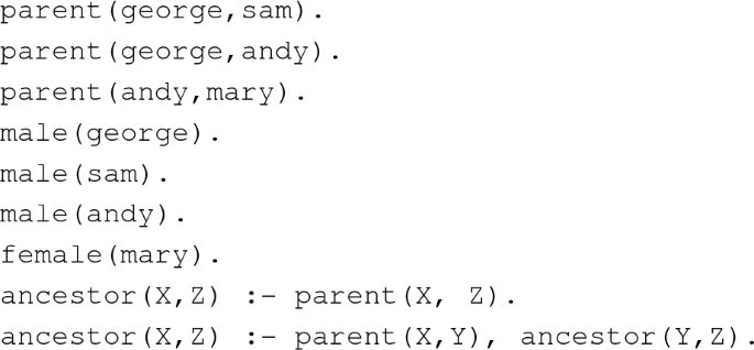
• 3. Given the following knowledge base for prolog, find a female descendant of ‘george’, by manually running the program.

  

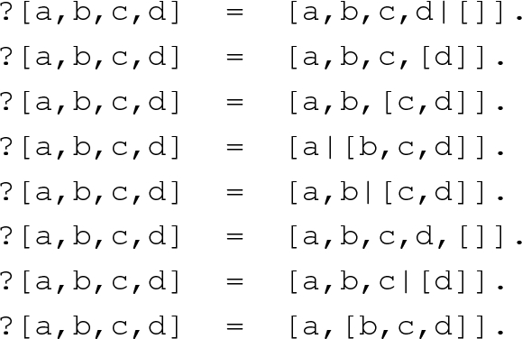
• 4. What is response of Prolog interpreter for following queries?

  

• 5. Which of the following lists are syntactically correct for Prolog language? Find out the number of elements in the lists that are correct.

  $\begin{array}{l} \left[ 1,2,3,4|\left[ \right] \right] \\ \left[ 1|\left[ 2|\left[ 3|\left[ 4\right] \right] \right] \right] \\ \left[ 1,2,3|\left[ \right] \right] \\ \left[ \left[ \right] |\left[ \right] \right] \\ \left[ \left[ 1,2\right] |4\right] \\ \left[ 1|\left[ 2,3,4\right] \right] \\ \left[ \left[ 1,2\right] ,\left[ 3,4\right] |\left[ 5,6,7\right] \right] \left[ 1|2,3,4\right] \\ \end{array}$

• 6. Write a predicate second(S, List), that checks whether S is the second element of List.

• 7. Consider the knowledge base comprising the the following facts:

  $\begin{array}{l} tran(ek,one).\\ tran(do,two).\\ tran(teen,three).\\ tran(char,four).\\ tran(panch,five).\\ tran(cha,six).\\ tran(saat,seven).\\ tran(aat,eight).\\ tran(no,nine).\\ \end{array}$

  Write a predicate listtran(H, E) that translates a list of Hindi number words to the corresponding list of English number words. For example, for a list X, listtran([ek, teen, chaar], X), should give response:

  $X = [one,three,four].$

• 8. Draw the search trees for the following prolog queries:

  • a. ?- member(x, [a, b, c]).

  • b. ?- member(a, [c, b, a, y]).

  • c. ?- member(X, [a, b, c]).

• 9. Write a program that takes a grammar represented as a list of rules and given a query of as sentence, and returns whether the sentence is grammatically correct.

• 10. Run the following programs in trace mode with single step, and describe the observed behavior, as why it is so?

  • a. Factorial Program (Example 5.5).

  • b. GCD Program (Example 5.6).

  • c. Mortal men program (Example 5.2).

• 11. Given the following facts and rules about a blocks world, represent them in rules forms, then translate the rules into prolog, and find out “what block is on black block?”

  • Facts:

  • A is on table.

  • B is on table.

  • E is on B.

  • C is on A.

  • C is heavy.

  • D has top clear.

  • E has top clear.

  • E is heavy.

  • C is iron made.

  • D is on C.

  • Rules:

  • Every big, black block is on a red block.

  • Every heavy, iron block is big.

  • All blocks with top clear are black.

  • All iron made blocks are black.

References

Clocksin WF, Mellish CS (2009) Programming in polog, 3rd edn. Narosa, New Delhi
http://www.dtic.upf.edu/~rramirez/lc/Prolog.pdf. Cited 19 Dec 2017
http://www.gprolog.org/. Cited 19 Dec 2017
Ivan B (2007) PROLOG programming for artificial intelligence, 3rd edn. Pearson Education
Strong John S (1989) The Legend of King Asoka—a study and translation of Asokavadana. Princeton University Press, Princeton, N.J.
Kowalski RA (1979) Algorithm = Logic + Control. Commun ACM 22(7):424–436
Van Emden MH, Kowalski RA (1976) The semantics of predicate logic as a programming language. J ACM 23(4):733–742
http://www.swi-prolog.org/. Cited 19 Dec 2017
Author information
Authors and Affiliations
Corresponding author