Supply Chain Analysis

Abstract

When starting an improvement process one has to have a clear picture of the structure of the existing supply chain and the way it works. Consequently a detailed analysis of operations and processes constituting the supply chain is necessary. Tools are needed that support an adequate description, modeling and evaluation of supply chains. In Sect. 2.1 some general topics relating to the motivation and objective of a supply chain analysis are discussed. Then, Sect. 2.2 presents modeling concepts and tools with a focus on those designed to analyze (supply chain) processes. The well known SCOR-model is introduced in this section. Building on these concepts (key) performance measures are presented in order to assess supply chain excellence (Sect. 2.3). Inventories are often built up at the interface between partners. As a seamless integration of partners is crucial to overall supply chain performance, a thorough analysis of these interfaces (i.e. inventories) is very important. Consequently, Sect. 2.4 gives an overview on inventories and introduces a standardized analysis methodology.

These keywords were added by machine and not by the authors. This process is experimental and the keywords may be updated as the learning algorithm improves.

When starting an improvement process one has to have a clear picture of the structure of the existing supply chain and the way it works. Consequently a detailed analysis of operations and processes constituting the supply chain is necessary. Tools are needed that support an adequate description, modeling and evaluation of supply chains. In Sect. 2.1 some general topics relating to the motivation and objective of a supply chain analysis are discussed. Then, Sect. 2.2 presents modeling concepts and tools with a focus on those designed to analyze (supply chain) processes. The well known SCOR-model is introduced in this section. Building on these concepts (key) performance measures are presented in order to assess supply chain excellence (Sect. 2.3). Inventories are often built up at the interface between partners. As a seamless integration of partners is crucial to overall supply chain performance, a thorough analysis of these interfaces (i.e. inventories) is very important. Consequently, Sect. 2.4 gives an overview on inventories and introduces a standardized analysis methodology.

1 Motivation and Goals

An accurate analysis of the supply chain serves several purposes and is more a continuous task than a one time effort. In today’s fast changing business environment, although a supply chain partnership is intended for a longer duration, supply chains keep evolving and changing to accommodate best to the customers’ needs. In the beginning or when a specific supply chain is analyzed for the first time in its entirety the result can be used as a starting point for improvement processes as well as a benchmark for further analyses. While the initial analysis itself often helps to identify potentials and opportunities it may well be used for target-setting, e.g. for APS implementation projects (see Chap. 15) to measure the benefit a successful implementation has provided. On the other hand, the supply chain analysis should evolve in parallel to the changes in the real world. In this way the associated performance measures keep track of the current state of the supply chain and may be used for supply chain controlling.

Many authors, researchers as wells as practitioners, thought about concepts and frameworks as well as detailed metrics to assess supply chain performance (see e.g. Dreyer 2000; Lambert and Pohlen 2001; Bullinger et al. 2002). In most concepts two fundamental interwoven tasks play an important role: process modeling and performance measurement. These two topics will be reviewed in detail in the following two sections, but beforehand some more general remarks will be made.

Supply chains differ in many attributes from each other (see also Chap. 3 for a detailed supply chain typology). A distinctive attribute often stressed in literature is the division into innovative product supply chains and functional product supply chains (see e.g. Fisher 1997; Ramdas and Spekman 2000). Innovative product supply chains are characterized by short product life cycles, unstable demands, but relatively high profit margins. This leads to a strong market orientation to match supply and demand as well as flexible supply chains to adapt quickly to market swings. On the contrary, functional product supply chains face a rather stable demand with long product life cycles, but rather low profit margins. These supply chains tend to focus on cost reductions of physical material flows and on value creating processes. Naturally, performance measures for both types of supply chains differ. Where time-to-market may be an important metric for innovative product supply chains, this metric does only have a minor impact when assessing performance of a functional product supply chain. Consequently, a supply chain analysis does not only have to capture the correct type of the supply chain, but should also reflect this in the performance measures to be evaluated. Supply chain’s visions or strategic goals should also mirror these fundamental concepts.

Furthermore, a meaningful connection between the process model and the underlying real world as well as between the process model and the performance measures is of utmost importance. Although participating companies are often still organized according to functions, the analysis of supply chains has to be process oriented. Therefore, it is essential to identify those units that contribute to the joint output. These units are then linked to the supply chain processes as well as to the cost accounting systems of the individual companies. Therefore, they can provide the link between the financial performance of the supply chain partners and the non-financial performance metrics which may be used for the whole supply chain.

Finally, a holistic view on the supply chain needs to be kept. This is especially true here, because overall supply chain costs are not necessarily minimized, if each partner operates at his optimum given the constraints imposed by supply chain partners. This is not apparent and will therefore be illustrated by means of an example. Consider a supplier-customer relationship which is enhanced by a vendor managed inventory (VMI) implementation. At the customer’s side the VMI implementation reduces costs yielding to a price reduction in the consumer market which is followed by a gain in market share for the product. Despite this success in the marketplace the supplier on the other hand may not be able to totally recover the costs he has taken off the shoulders of his customer. Although some cost components decreased (e.g. order processing costs and costs of forecasts), these did not offset his increased inventory carrying costs. Summing up, although the supply chain as a whole profited from the VMI implementation, one of the partners was worse off. Therefore, when analyzing supply chains one needs to maintain such a holistic view, but simultaneously mechanisms need to be found to compensate those partners that do not profit directly from supply chain successes.

2 Process Modeling

2.1 Concepts and Tools

Supply chain management’s process orientation has been stressed before and since Porter’s introduction of the value chain a paradigm has been developed in economics that process oriented management leads to superior results compared to the traditional focus on functions. When analyzing supply chains, the modeling of processes is an important first cornerstone. In this context several questions arise. First, which processes are important for the supply chain and second, how can these processes be modeled.

To answer the first question, the Global Supply Chain Forum identifies eight core supply chain processes (Croxton et al. 2001):

• Customer relationship management

• Customer service management

• Demand management

• Order fulfillment

• Manufacturing flow management

• Supplier relationship management (procurement)

• Product development and commercialization

• Returns management (returns).

Although the importance of each of these processes as well as the activities/operations performed within these processes may vary between different supply chains, these eight processes make up an integral part of the business to be analyzed. Both, a strategic view, especially during implementation, and an operational view have to be taken on each of these processes. Figure 2.1 gives an example for the order fulfillment process and shows the sub-processes for either view as well as potential interferences with the other seven core processes.

Fig. 2.1

Order fulfillment process (Croxton et al. 2001, p. 21)

Going into more detail, processes can be traced best by the flow of materials and information flows. For example, a flow of goods (material flow) is most often initiated by a purchase order (information flow) and followed by an invoice and payment (information and financial flow) to name only a few process steps. Even though several functions are involved: purchasing as initiator, manufacturing as consumer, logistics as internal service provider and finance as debtor. Furthermore, these functions interact with corresponding functions of the supplier. When analyzing supply chains the material flow (and related information flows) need to be mapped from the point of origin to the final customer and probably all the way back, if returns threaten to have a significant impact. Special care needs to be taken at the link between functions, especially when these links bridge two companies, i.e. supply chain members. Nonetheless, a functional view can be helpful when structuring processes.

Furthermore, the process models can serve a second purpose. They may be used to simulate different scenarios by assigning each process chain element certain attributes (e.g. capacities, process times, availability) and then checking for bottlenecks (Arns et al. 2002). At this point simulation can help to validate newly designed processes and provide the opportunity to make process changes well in time.

The by far most widespread process model especially designed for modeling of supply chains is the SCOR-model which will therefore be presented in more detail.

2.2 The SCOR-Model

The Supply Chain Operations Reference (SCOR-)model (current version is 11.0) is a tool for representing, analyzing and configuring supply chains. The SCOR-model has been developed by the Supply-Chain Council (SCC) founded in 1996 as a non-profit organization by AMR Research, the consulting firm Pittiglio Rabin Todd & McGrath (PRTM) and 69 companies. In 2012 SCC had close to 1,000 corporate members (Supply Chain Council 2014).

The SCOR-model is a reference model. It does not provide any optimization methods, but aims at providing a standardized terminology for the description of supply chains. This standardization allows benchmarking of processes and the extraction of best practices for certain processes. The relevance of the SCOR model for current supply chain performance measurement has also been confirmed in a literature review by Akyuz and Erkan (2010, p. 5152).

2.2.1 Standardized Terminology

Often in different companies different meanings are associated with certain terms. The less one is aware upon the different usage of a term, the more likely misconceptions occur. The use of a standardized terminology that defines and unifies the used terms improves the communication between entities of a supply chain. Thereby, misconceptions are avoided or at least reduced. SCC has established a standard terminology within its SCOR-model.

2.2.2 Levels of the SCOR-Model

The SCOR-model consists of a system of process definitions that are used to standardize processes relevant for SCM. SCC recommends to model a supply chain from the suppliers’ suppliers to the customers’ customers. Processes such as customer interactions (order entry through paid invoice), physical material transactions (e.g. equipment, supplies, products, software), market interactions (e.g. demand fulfillment), returns management and (since release 11.0) enable processes are supported. Sales and marketing as well as product development and research are not addressed within the SCOR-model (Supply Chain Council 2012, p. i.2).

The standard processes are divided into four hierarchical levels : process types, process categories, process elements and implementation. The SCOR-model only covers the upper three levels, which will be described in the following paragraphs (following Supply Chain Council 2012, pp. 2.0.1–2.6.84), while the lowest (implementation) level is out of the scope of the model, because it is too specific for each company.

2.2.2.1 Level 1: Process Types

Level 1 consists of the six elementary process types: plan, source, make, deliver, return and enable. These process types comprise operational as well as strategic activities (see Chap. 4). The description of the process types follows Supply Chain Council (2012).

Plan .:

Plan covers processes to balance resource capacities with demand requirements and the communication of plans across the supply chain. Also in its scope are measurement of the supply chain performance and management of inventories, assets and transportation among others.

Source .:

Source covers the identification and selection of suppliers, measurement of supplier performance as well as scheduling of their deliveries, receiving of products and processes to authorize payments. It also includes the management of the supplier network and contracts as well as inventories of delivered products.

Make .:

In the scope of make are processes that transform material, intermediates and products into their next state, meeting planned and current demand. Make covers processes to schedule production activities, produce and test, packaging as well as release of products for delivery. Furthermore, make covers the management of in-process products (WIP), equipment and facilities.

Deliver .:

Deliver covers processes like order reception, reservation of inventories, generating quotations, consolidation of orders, load building and generation of shipping documents and invoicing. Deliver includes all steps necessary for order management, warehouse management and reception of products at a customer’s location together with installation. It manages finished product inventories, service levels and import/export requirements.

Return .:

In the scope of return are processes for returning defective or excess supply chain products as well as MRO products. The return process extends the scope of the SCOR-model into the area of post-delivery customer service. It covers the authorization of returns, scheduling of returns, receiving and disposition of returned products as well as replacements or credits for returned products. In addition return manages return inventories as well as the compliance to return policies.

Enable .:

The enable processes support the planning and execution of the above supply chain processes. Enable processes are related to maintaining and monitoring of information, resources, compliance and contracts that govern the operation of the supply chain. Therefore enable processes interact with other domains, ranging from HR processes to financial processes and sales and support processes.

2.2.2.2 Level 2: Process Categories

The six process types of level 1 are decomposed into 30 process categories, including nine enable process categories (see Table 2.1). The second level deals with the configuration of the supply chain. At this level typical redundancies of established businesses, such as overlapping planning processes and duplicated purchasing, can be identified. Delayed customer orders indicate a need for integration of suppliers and customers.

Table 2.1 Process categories

Process types	Return	Enable
Process categories	sSR1: Source return defective product	sE1: Manage business rules
	sDR1: Deliver return defective product	sE2: Manage performance
	sSR2: Source return MRO product	sE3: Manage data and information
	sDR2: Deliver return MRO product	sE4: Manage human resources
	sSR3: Source return excess product	sE5: Manage assets
	sDR3: Deliver return excess product	sE6: Manage contracts
		sE7: Manage networks
		sE8: Manage regulatory compliance
		sE9: Manage risk

2.2.2.3 Level 3: Process Elements

At this level, the supply chain is tuned. The process categories are further decomposed into process elements. Detailed metrics and best practices for these elements are part of the SCOR-model at this level. Furthermore, most process elements can be linked and possess an input stream (information and material) and/or an output stream (also information and material). Figure 2.2 shows an example for the third level of the “sP1: Plan supply chain” process category. Supply Chain Council (2012, pp. 2.1.2–2.1.11) gives the following definitions for this process category and its process elements:

Fig. 2.2

Example of SCOR-model’s level 3 (based on Supply Chain Council 2012)

“sP1. :

The development and establishment of courses of action over specified time periods that represent a projected appropriation of supply chain resources to meet supply chain requirements for the longest time fence constraints of supply resources.

sP1.1. :

The process of identifying, aggregating and prioritizing, all sources of demand for the integrated supply chain of a product or service at the appropriate level, horizon and interval.

sP1.2. :

The process of identifying, prioritizing, and aggregating, as a whole with constituent parts, all sources of the supply chain that are required and add value in the supply chain of a product or service at the appropriate level, horizon and interval.

sP1.3. :

The process of identifying and measuring the gaps and imbalances between demand and resources in order to determine how to best resolve the variances through marketing, pricing, packaging, warehousing, outsource plans or some other actions that will optimize service, flexibility, costs, assets, (or other supply chain inconsistencies) in an iterative and collaborative environment.

sP1.4. :

The establishment and communication of courses of action over the appropriate time-defined (long-term, annual, monthly, weekly) planning horizon and interval, representing a projected appropriation of supply-chain resources to meet supply chain requirements.”

The input and output streams of a process element are not necessarily linked to input and output streams of other process elements. However, the indication in brackets depicts the corresponding supply chain partner, process type, process category or process element from where information or material comes. Thus, the process elements are references, not examples of possible sequences.

The process elements are decomposed on the fourth level. Companies implement their specific management practices at this level. Not being part of the SCOR-model, this step will not be subject of this book.

2.2.3 Metrics and Best Practices

The SCOR-model supports performance measurement on each level. Level 1 metrics provide an overview of the supply chain for the evaluation by management (see Table 2.2). Levels 2 and 3 include more specific and detailed metrics corresponding to process categories and elements. Table 2.3 gives an example of level 3 metrics that are corresponding to the “sS1.1: Schedule product deliveries” process element.

Table 2.2 SCOR’s level 1 metrics (Supply Chain Council 2012, p. 1.0.2)

Table 2.3 SCOR’s level 3 metrics—example “sS1.1: Schedule product deliveries” (Supply Chain Council 2012, p. 2.2.5)

The metrics are systematically divided into the five categories reliability, responsiveness, agility, cost and asset management efficiency. Reliability as well as agility and responsiveness are external (customer driven), whereas cost and asset management efficiency are metrics from an internal point of view.

In 1991 PRTM initiated the Supply Chain Performance Benchmarking Study (now: Supply-Chain Management Benchmarking Series) for SCC members (Stewart 1995). Within the scope of this study all level 1 metrics and selected metrics of levels 2 and 3 are gathered. This information is evaluated with respect to different lines of business. Companies joining the Supply Chain Performance Benchmarking Study are able to compare their metrics with the evaluated ones. Furthermore, associated best practices are identified. Selected best practices, corresponding to process categories and process elements, are depicted in the following paragraph.

An example of an identified best practice for the “sP1: Plan supply chain” process category is high integration of the supply/demand process from gathering customer data and order receipt, through production to supplier request. SCC recommends performing this integrated process by using an APS with interfaces to all supply/demand resources. Moreover, the utilization of tools that support balanced decision-making (e.g. trade-off between service level and inventory investment) is identified as best practice. To perform process element “sP1.3: Balance supply chain resources with supply chain requirements” (see Fig. 2.2) effectively, balancing of supply and demand to derive an optimal combination of customer service and resource investment by using an APS is recognized as best practice (e.g. BP.086—Supply Network Planning, Supply Chain Council 2012, p. 3.2.70).

2.2.4 A Procedure for Application of the SCOR-Model

Having described the elements of the SCOR-model, a procedure for its application will be outlined that shows how the SCOR-model can be configured for a distinct supply chain (adapted from Supply Chain Council 2007, pp. 19–21). This configuration procedure consists of seven steps:

• 1. Define the business unit to be configured.

• 2. Geographically place entities that are involved in source, make, deliver and return process types. Not only locations of a single business, but also locations of suppliers (and suppliers’ suppliers) and customers (and customers’ customers) should be denoted.

• 3. Enter the major flows of materials as directed arcs between locations of entities.

• 4. Assign and link the most important source, make, deliver and return processes categories to each location (see Fig. 2.3).

  Fig. 2.3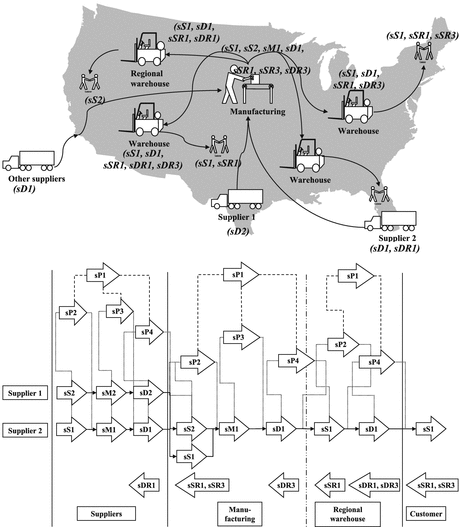

  

  Example results of steps 4 and 6 (adapted from Supply Chain Council 2007, pp. 19–21)

• 5. Define partial process chains of the (modeled) supply chain (e.g. for distinct product families). A partial process chain is a sequence of processes that are planned for by a single “sP1” planning process category.

• 6. Enter planning process categories (“sP2”–“sP5”) using dashed lines to illustrate the assignment of execution to planning process categories (see Fig. 2.3).

• 7. Define a top-level “sP1” planning process if possible, i.e. a planning process category that coordinates two or more partial process chains.

The result of step 4 is a map that shows the material flows in a geographical context, indicating complexity or redundancy of any nodes. The result of step 7 is a thread diagram that focuses on the level 2 (process categories) to describe high-level process complexity or redundancy. After configuring the supply chain, performance levels, practices and systems are aligned. Critical process categories of level 2 can be detailed in level 3. At this level the most differentiated metrics and best practices are available. Thus, detailed analysis and improvements of process elements are supported.

The implementation of supply chain processes and systems is, as already mentioned, not part of the SCOR-model. However, it is recommended to continue to use the metrics of the SCOR-model. They provide data for internal and external benchmarking studies to measure and document consequences of change processes within a supply chain.

3 Performance Measurement

Having mapped the supply chain processes it is important to assign measures to these processes to evaluate changes and to assess the performance of the complete supply chain as well as of the individual processes. Thereby it is crucial not to measure “something”, but to find the most relevant metrics. These not only need to be aligned with the supply chain strategy (see Sect. 1.2.4), but also need to reflect important goals in the scope and within the influence of the part of the organization responsible for the individual process under consideration. Furthermore the identification of changes in the structure or the type of the supply chain (see Chap. 3) has to be supported. In the next two subsections, first some general topics related to performance measurement within a supply chain setting will be discussed, and afterwards key performance indicators for supply chains will be introduced.

3.1 General Remarks

Indicators are defined as numbers that inform about relevant criteria in a clearly defined way (see e.g. Horváth 2011 for a comprehensive introduction to indicators and systems of indicators). Performance indicators (measures , metrics ) are utilized in a wide range of operations. Their primary application is in operational controlling. Hardly a controlling system is imaginable that does not make use of performance measures regularly. In fact, the utilization of a wide variety of measures (as necessary) to model all business processes of a company enables the company to run its business according to management-by-exception.

Three functions can be attributed to indicators :

Informing. :

Their main purpose is to inform management. In this function, indicators are applied to support decision-making and to identify problem areas. Indicators can therefore be compared with standard or target values.

Steering. :

Indicators are the basis for target setting. These targets guide those responsible for the process considered to accomplish the desired outcome.

Controlling. :

Indicators are also well suited for the supervision of operations and processes.

The main disadvantage inherent to indicators is that they are only suited to describe quantitative facts. “Soft” facts are difficult to measure and likely to be neglected when indicators are introduced (e.g. motivation of personnel). Still, non-quantitative targets which are not included in the set of indicators should be kept in mind.

When using indicators, one key concern is their correct interpretation. It is essential to keep in mind that variations observed by indicators have to be linked to a causal model of the underlying process or operation. A short example will illustrate this. To measure the productivity of an operation the ratio of revenue divided by labor is assumed here as an appropriate indicator:

$$\displaystyle{ \text{productivity} = \frac{\text{revenue}[\$]} {\text{labor}[\text{h}]} }$$

(2.1)

Revenue is measured in currency units ($), whereas labor is measured in hours worked (per plant, machine or personnel), where the relevance of the different measures for labor depends on the specific product(s) considered. Supposed productivity is 500$/h in one period and 600$/h in the next period, there is definitely a huge difference. In fact, when calculating productivity a causal link between revenue and labor is assumed implicitly. On the other hand, there are many more rationales that could have caused this increase in productivity. These have to be examined too before a final conclusion can be derived. In this example price hikes, changes in product mix, higher utilization of resources or decreased inventories can account for substantial portions of the observed increase in productivity. Therefore, it is essential to find appropriate measures with clear links connecting the indicator and the causal model of the underlying process (root causes).

Furthermore, indicators have to be evaluated how they translate to the strategic goals of the supply chain. If indicators and strategy are not aligned, it may well happen that one supply chain entity pursues a conflicting goal. For example, one partner increases its inventory turn rate by reducing safety stock, which negatively affects the downstream delivery performance of its partners.

When choosing supply chain performance metrics it is essential to keep in mind the cross-functional process-oriented nature of the supply chain. Functional measures may be to narrow-minded and should be substituted by cross-functional measures, therefore helping that not individual entities optimize only their functional goals (e.g. maximizing capacity utilization), but shared goals (e.g. a superior order fill rate compared to a rival supply chain).

Historically, indicators and systems of indicators have been based on financial data, as financial data have been widely available for long. Improvements in terms of superior financial performance that are caused by the successful application of SCM can be measured by these indicators. Nevertheless some additional, more appropriate measures of supply chain performance should be derived, since the focal points of SCM are customer orientation, the integration of organizational units and their coordination.

The transition to incorporate non-financial measures in the evaluation of business performance is widely accepted, though. Kaplan and Norton (1992) introduced the concept of a balanced scorecard (BSC) that received broad attention not only in scientific literature but also in practical applications. In addition to financial measures, the BSC comprises a customer perspective, an innovation and learning perspective as well as an internal business perspective. These perspectives integrate a set of measures into one management report that provides a deeper insight into a company’s performance. The measures chosen depend on the individual situation faced by the company. Figure 2.4 gives an example of a BSC used by a global engineering and construction company.

Fig. 2.4

Example of indicators used by a balanced scorecard (Kaplan and Norton 1993, p. 136)

An increasing number of contributions in the literature is dealing with the adaptation of BSCs to fit the needs of SCM (see e.g. Brewer and Speh 2000; Bullinger et al. 2002; Richert 2006). Adaptations are proposed within the original framework consisting of the four perspectives introduced above, but also structural changes are proposed. For example, Weber et al. (2002) propose a BSC for supply chains consisting of a financial perspective, a process perspective and two new perspectives relating to cooperation quality and cooperation intensity. In addition to the supply chain BSC they propose individual company BSCs on a second hierarchical level. In contrast to the supply chain BSC these still might comprise of a customer perspective (for the most downstream supply chain partner) and a learning perspective.

Non-financial measures have the advantage that they are often easier to quantify as there is no allocation of costs necessary for their calculation. Moreover, they turn attention to physical processes more directly. An instrument providing connections of root causes and financial performance measures via non-financial/logistical key performance indicators are the Enabler-KPI-Value networks presented in Chap. 15.

Specifically when assessing supply chain performance it is important to bear in mind the following:

Definition of Indicators. :

As supply chains usually span over several companies or at least several entities within one company a common definition of all indicators is obligatory. Otherwise the comparison of indicators and their uniform application can be counterproductive.

Perspective on Indicators. :

The view on indicators might be different considering the roles of the two supply chain partners, the supplier and the customer. A supplier might want to calculate the order fill rate based on the order receipt date and the order ship date, as these are the dates he is able to control. From the customer’s point of view the basis would be the request date and the receipt date at customer’s warehouse. If supplier’s and customer’s dates do not match, this will lead to different results with respect to an agreed order fill rate. This is why both have to agree on one perspective.

Capturing of Data. :

Data needed to calculate the indicators should be captured in a consistent way throughout the supply chain. Consistency with respect to units of measurement and the availability of current data for the supply chain partners are essential. Furthermore, completeness of the used data is obligatory, i.e. all necessary data should be available in adequate systems and accessible by supply chain partners.

Relevance of Indicators. :

Due to the enormous number of indicators available the identification of a most selective subset is important to control the specific object or situation at best without wasting a lot of effort in analyzing useless data.

Big Data. :

“Big data refers to datasets whose size is beyond the ability of typical database software tools to capture, store, manage, and analyze” (Manyika et al. 2011, p. 1). The amount of data is exponentially increasing and changing over time thus analyzing e.g. forecast accuracy comparing several years of granular sales data compared to monthly released rolling sales forecasts leads to billions of data records. Combining the structured data from data bases with unstructured data like comments explaining a specific situation becomes a challenge.

Confidentiality. :

Confidentiality is another major issue if more than one company form the supply chain. As all partners are separate legal entities, they might not want to give complete information about their internal processes to their partners. Furthermore, there might be some targets which are not shared among partners.

Nevertheless, it is widely accepted that supply chain integration benefits from the utilization of key performance indicators. They support communication between supply chain partners and are a valuable tool for the coordination of their individual, but shared plans. Additional findings related to the problems with today’s performance management systems, requirements for performance measurement metrics, the importance of the balanced scorecard approach and the SCOR model and the importance of the “concept of fit” in supply chain performance measurement can be found in the literature review by Akyuz and Erkan (2010).

3.2 Key Performance Indicators for Supply Chains

A vast amount of literature has been published suggesting performance indicators for supply chains (e.g. Lapide 2000; Gunasekaran et al. 2001; Bullinger et al. 2002; Hausman 2003). A supply chain benchmarking study undertaken with 148 supply chain managers in Germany, Switzerland and Austria from different industries analyzed the importance of SCOR’s performance attributes and several KPIs used to measure supply chains’ performance. The sorting of attributes shows that a majority of the participants put reliability on the first position, followed by agility/flexibility, responsiveness and costs (see Fig. 2.5). Assets are considered to be less important. Apart from the “typical” metrics supporting SCOR’s performance attributes the study also analyzed the importance of metrics related with supply chain risks (e.g. security of supply, bad debt, cancellations) and sustainability (e.g. carbon footprint, renewable energies). Disasters like Fukushima in 2011 might have an impact on a changed perception but the ranking of the metrics shows that both categories are of minor relevance (Reuter 2013, p. 50).

Fig. 2.5

KPIs and categories—comparison based on Reuter (2013, p. 50)

Although each supply chain is unique and might need special treatment, there are some performance measures that are applicable in most settings. In the following paragraphs these will be presented as key performance indicators. As they tackle different aspects of the supply chain they are grouped into four categories corresponding to the following attributes: delivery performance, supply chain responsiveness, assets and inventories, and costs.

3.2.1 Delivery Performance

As customer orientation is a key component of SCM, delivery performance is an essential measure for total supply chain performance. As promised delivery dates may be too late in the eye of the customer, his expectation or even request determines the target. Therefore delivery performance has to be measured in terms of the actual delivery date compared to the delivery date mutually agreed upon. Only perfect order fulfillment which is reached by delivering the right product to the right place at the right time ensures customer satisfaction. An on time shipment containing only 95 % of items requested will often not ensure 95 % satisfaction with the customer. Increasing delivery performance may improve the competitive position of the supply chain and generate additional sales. Regarding different aspects of delivery performance, various indicators called service levels are distinguished in inventory management literature (see e.g. Tempelmeier 2005, pp. 27–29 or Silver et al. 1998, p. 245). The first one, called α-service level (P₁, cycle service level), is an event-oriented measure. It is defined as the probability that an incoming order can be fulfilled completely from stock. Usually, it is determined with respect to a predefined period length (e.g. day, week or order cycle). Another performance indicator is the quantity-oriented β-service level (P₂), which is defined as the proportion of incoming order quantities that can be fulfilled from inventory on-hand. In contrast to the α-service level, the β-service level takes into account the extent to which orders cannot be fulfilled. The γ-service level is a time- and quantity-oriented measure. It comprises two aspects: the quantity that cannot be met from stock and the time it takes to meet the demand. Therefore it contains the time information not considered by the β-service level. An exact definition is:

$$\displaystyle\begin{array}{rcl} \gamma \text{-service level}& =& 1 -\frac{\text{mean backlog at end of period }} {\text{mean demand per period }}{}\end{array}$$

(2.2)

Furthermore, on time delivery is an important indicator. It is defined as the proportion of orders delivered on or before the date requested by the customer. A low percentage of on time deliveries indicates that the order promising process is not synchronized with the execution process. This might be due to order promising based on an infeasible (production) plan or because of production or transportation operations not executed as planned.

Measuring forecast accuracy is also worthwhile. Forecast accuracy relates forecasted sales quantities to actual quantities and measures the ability to forecast future demands. Better forecasts of customer behavior usually lead to smaller changes in already established production and distribution plans. An overview of methods to measure forecast accuracy is given in Chap. 7.

Another important indicator in the context of delivery performance is the order lead-time . Order lead-times measure, from the customer’s point of view, the average time interval from the date the order is placed to the date the customer receives the shipment. As customers are increasingly demanding, short order lead-times become important in competitive situations. Nevertheless, not only short lead-times but also reliable lead-times will satisfy customers and lead to a strong customer relationship, even though the two types of lead-times (shortest vs. reliable) have different cost aspects.

3.2.2 Supply Chain Responsiveness

Responsiveness describes the ability of the complete supply chain to react according to changes in the marketplace. Supply chains have to react to significant changes within an appropriate time frame to ensure their competitiveness. To quantify responsiveness separate flexibility measures have to be introduced to capture the ability, extent and speed of adaptations. These indicators shall measure the ability to change plans (flexibility within the system) and even the entire supply chain structure (flexibility of the system). An example in this field is the upside production flexibility determined by the number of days needed to adapt to an unexpected 20 % growth in the demand level.

A different indicator in this area is the planning cycle time which is simply defined as the time between the beginning of two subsequent planning cycles. Long planning cycle times prevent the plan from taking into account the short-term changes in the real world. Especially planned actions at the end of a planning cycle may no longer fit to the actual situation, since they are based on old data available at the beginning of the planning cycle. The appropriate planning cycle time has to be determined with respect to the aggregation level of the planning process, the planning horizon and the planning effort.

3.2.3 Assets and Inventories

Measures regarding the assets of a supply chain should not be neglected. One common indicator in this area is called asset turns, which is defined by the division of revenue by total assets. Therefore, asset turns measure the efficiency of a company in operating its assets by specifying sales per asset. This indicator should be watched with caution as it varies sharply among different industries.

Another indicator worthy of observation is inventory turns , defined as the ratio of total material consumption per time period over the average inventory level of the same time period. A common approach to increase inventory turns is to reduce inventories. Still, inventory turns is a good example to illustrate that optimizing the proposed measures may not be pursued as isolated goals. Consider a supply chain consisting of several tiers each holding the same quantity of goods in inventory. As the value of goods increases as they move downstream the supply chain, an increase in inventory turns is more valuable if achieved at a more downstream entity. Furthermore, decreasing downstream inventories reduces the risk of repositioning of inventories due to bad distribution. However, reduced inventory holding costs may be offset by increases in other cost components (e.g. production setup costs) or unsatisfied customers (due to poor delivery performance). Therefore, when using this measure it needs to be done with caution, keeping a holistic view on the supply chain in mind.

Lastly, the inventory age is defined by the average time goods are residing in stock. Inventory age is a reliable indicator for high inventory levels, but has to be used with respect to the items considered. Replacement parts for phased out products will usually have a much higher age than stocks of the newest released products. Nevertheless, the distribution of inventory ages over products is suited perfectly for identifying unnecessary “pockets” of inventory and for helping to increase inventory turns.

Determining the right inventory level is not an easy task, as it is product- and process-dependent. Furthermore, inventories not only cause costs, but there are also benefits to holding inventory. Therefore, in addition to the aggregated indicators defined above, a proper analysis not only regarding the importance of items (e.g. an ABC-analysis), but also a detailed investigation of inventory components (as proposed in Sect. 2.4) might be appropriate.

3.2.4 Costs

Last but not least some financial measures should be mentioned since the ultimate goal will generally be profit. Here, the focus is on cost based measures. Costs of goods sold should always be monitored with emphasis on substantial processes of the supply chain. Hence, an integrated information system operating on a joint database and a mutual cost accounting system may prove to be a vital part of the supply chain.

Further, productivity measures usually aim at the detection of cost drivers in the production process. In this context value-added employee productivity is an indicator which is calculated by dividing the difference between revenue and material cost by total employment (measured in (full time) equivalents of employees). Therefore, it analyses the value each employee adds to all products sold.

Finally, warranty costs should be observed, being an indicator for product quality. Although warranty costs depend highly on how warranty processing is carried out, it may help to identify problem areas. This is particularly important because superior product quality is not a typical supply chain feature, but a driving business principle in general.

4 Inventory Analysis

Often claimed citations like “inventories hide faults” suggest to avoid any inventory in a supply chain. This way of thinking is attributed to the Just-In-Time-philosophy, which aligns the processes in the supply chain such that almost no inventories are necessary. This is only possible in some specific industries or certain sections of a supply chain and for selected items.

In all other cases inventories are necessary and therefore need to be managed in an efficient way. Inventories in supply chains are always the result of inflow and outflow processes (transport, production etc.). This means that the isolated minimization of inventories is not a reasonable objective of SCM, instead they have to be managed together with the corresponding supply chain processes.

Inventories cause costs (holding costs), but also provide benefits, in particular reduction of costs of the inflow and/or outflow processes. Thus, the problem is to find the right trade-off between the costs for holding inventories and the benefits.

Inventory decomposes into different components according to the motives for holding inventory. The most important components are shown in Table 2.4 and will be described in detail in the following paragraphs.

Table 2.4 Stock components, determinants, and benefits

The distinction of stock components is necessary for

• The identification of benefits

• The identification of determinants of the inventory level

• Setting target inventory levels (e.g. in APS).

The inventory analysis enables us to decompose the average inventory level in a supply chain. It shows the different causes for inventories held in the past and indicates the relative importance of specific components. The current inventory of certain stock keeping units (SKUs) on the other hand might be higher or lower depending on the point in time chosen. Thus, the current inventory is not suitable for a proper inventory analysis.

In an ex-post analysis it is possible to observe whether the trade-off between the benefits and the stock costs has been managed efficiently for each component and SKU (inventory management). In the following paragraphs we will show the motives, the benefits, and determinants of some important components (see also Chopra and Meindl 2007, p. 50).

4.1 Production Lot-Sizing or Cycle Stock

The cycle stock (we use ‘production lot-sizing stock’, ‘lot-sizing stock’ and ‘cycle stock’ synonymously) is used to cover the demand between two consecutive production runs of the same product. For example, consider a color manufacturing plant, which produces blue and yellow colors, alternating between each bi-weekly. Then, the production lot has to cover the demand in the current and the following week. Thus, the production quantity (lot) equals the 2-week demand and the coverage is 2 weeks. The role of cycle stock is to reduce the costs for setting up and cleaning the production facility (setup or changeover costs). Finding the right trade-off between fixed setup costs and inventory costs is usually a critical task, as this decision may also depend on the lot-size of other products. An overview on the problems arising here is given in Chap. 10.

For the inventory analysis of final items in a make-to-stock environment it is mostly sufficient to consider a cyclic production pattern with average lot-sizes q ^p over a time interval that covers several production cycles. Then, the inventory level follows the so-called “saw-tooth”-pattern, which is shown in Fig. 2.6.

Fig. 2.6

Inventory pattern for cycle stock calculation

The average cycle stock CS is half the average lot-size: $\mathit{CS} = q^{p}/2$. The average lot-size can be calculated from the total number of production setups su and the total demand d ^p during the analysis interval: $q^{p} = d^{p}/\mathit{su}$. Thus, all you need to analyze cycle stock is the number of production setups and the total demand.

4.2 Transportation Lot-Sizing Stock

The same principle of reducing the amount of fixed costs per lot applies to transportation links. Each truck causes some amount of fixed costs which arise for a transport from warehouse A to warehouse B. If this truck is only loaded partially, then the cost per unit shipped is higher than for a full truckload. Therefore, it is economical to batch transportation quantities up to a full load and to ship them together. Then, one shipment has to cover the demand until the next shipment arrives at the destination. The decision on the right transportation lot-size usually has to take into account the dependencies with other products’ shipments on the same link and the capacity of the transport unit (e.g. truck, ship etc.) used (see Chap. 12).

For the inventory analysis we can calculate the average transportation quantity q ^t from the number of shipments s during the analysis interval and the total demand d ^t for the product at the destination warehouse by $q^{t} = d^{t}/s$. In contrast to the production lot-sizing stock, the average transportation lot-sizing stock equals not half, but the whole transportation quantity q ^t, if we consider both the “source warehouse”, where the inventory has to be built up until the next shipment starts and the “destination warehouse” where the inventory is depleted until the next shipment arrives. Therefore, the average stock level at each warehouse is one half of the transportation lot-size and, the transportation lot-sizing stock sums up to TLS = q ^t.

This calculation builds on the assumption of a continuous inflow of goods to the source warehouse, which is valid if the warehouse is supplied by continuous production or by production lots which are not coordinated with the shipments. This is the case for most production-distribution chains.

4.3 Inventory in Transit

While the transportation lot-sizing stock is held at the start and end stock points of a transportation link, there exists also inventory that is currently transported in-between. This stock component only depends on the transportation time and the demand because on average the inventory “held on the truck” equals the demand which occurs during the transportation time. The inventory in transit is independent of the transportation frequency and therefore also independent of the transportation lot-size. The inventory in transit can be reduced at the expense of increasing transportation costs, if the transportation time is reduced by a faster transportation mode (e.g. plane instead of truck transport).

The average inventory in transit TI is calculated by multiplying the average transportation time by the average demand. For instance, if the transportation time is 2 days and the average amount to be transported is 50 pieces per day, then TI = 100 pieces.

4.4 Seasonal Stock or Pre-built Stock

In seasonal industries (e.g. consumer packaged goods) inventories are held to buffer future demand peaks which exceed the production capacities. In this sense, there is a trade-off between the level of regular capacity, additional overtime capacity and seasonal stock. The seasonal stock can help to reduce lost sales, costs for working overtime or opportunity costs for unused machines and technical equipment. In contrast to the previous stock components which are defined by SKU, the seasonal stock is common for a group of items sharing the same tight capacity. Figure 2.7 shows how the total amount of seasonal inventory can be calculated from the capacity profile of a complete seasonal cycle.

Fig. 2.7

Example for the determination of seasonal stock

In this case, the seasonal stock is built up in periods 3 and 4 and used for demand fulfillment in periods 6 and 7. The total seasonal stock shown in the figure is calculated using the assumption that all products are pre-produced in the same quantity as they are demanded in the bottleneck periods. In practice one would preferably pre-build those products, which create only small holding costs and which can be forecasted with high certainty. In Chap. 8 we will introduce planning models, which help to decide on the right amount of seasonal stock.

4.5 Work-in-Process Inventory (WIP)

The WIP inventory can be found in every supply chain, because the production process takes some time during which the raw materials and components are transformed to finished products. In a multi-stage production process the production lead time consists of the actual processing times on the machines and additional waiting times of the products between the operations, e.g. because required resources are occupied. The benefits of the WIP are that it prevents bottleneck machines from starving for material and maintains a high utilization of resources. Thus, WIP may avoid investments in additional capacities. The waiting time part of production lead time is also influenced by the production planning and control system (see also Chap. 10), which should schedule the orders so as to ensure short lead times. Therefore, it is possible to reduce the WIP by making effective use of an APS. In this sense, the opinion “inventories hide faults” indeed applies to the WIP in the modified form: Too high WIP hides faults of production planning and control.

According to Little’s law (see e.g. Silver et al. 1998, p. 697) the average production lead time LT is proportional to the WIP level. If d ^w is the average demand per unit of time, then WIP = LT ⋅ d ^w.

4.6 Safety Stock

Safety stock has to protect against uncertainty which may arise from internal processes like production lead time, from unknown customer demand and from uncertain supplier lead times. This implies that the main drivers for the safety stock level are production and transport disruptions, forecasting errors, and lead time variations. The benefit of safety stock is that it allows quick customer service and avoids lost sales, emergency shipments, and the loss of goodwill. Furthermore, safety stock for raw materials enables smoother flow of goods in the production process and avoids disruptions due to stock-outs at the raw material level. Besides the uncertainty mentioned above the main driver for safety stock is the length of the lead time (production or procurement), which is necessary to replenish the stock.

In the inventory analysis, the observed safety stock is the residual level, which is left after subtracting all of the components introduced above from the average observed inventory level. This observed safety stock can then be compared with the level of safety stock that is necessary from an economical standpoint. A short introduction on how necessary safety stocks can be calculated is given in Chap. 7.

A further component which may occur in a distribution center is the order picking inventory . It comprises the partly filled pallets from which the small quantities per customer order are picked.

The main steps of the inventory analysis are summarized in the following:

• 1. Calculate the average inventory level (AVI) from past observations over a sufficiently long period (e.g. half a year) of observations (e.g. inventory levels measured daily or weekly).

• 2. Identify possible stock components (e.g. cycle stock, safety stock) and their corresponding drivers (e.g. lot-size, lead time).

• 3. Decompose the AVI into the components including the observed safety stock.

• 4. Calculate the necessary safety stock and compare it to the observed safety stock.

• 5. The remaining difference ($+/-$) shows avoidable buffer stock (+) or products which didn’t have enough stock (−).

• 6. For the most important components of the observed inventory calculate the optimal target level w. r. t. inventory costs and benefits.

For the optimization of inventory, the main principle of inventory management has to be considered: The objective is to balance the costs arising from holding inventories and the benefits of it. Furthermore, this trade-off has to be handled for each separate component. In Part II we will show how APS can support this critical task of inventory management.

References

Akyuz, G. A., & Erkan, T. E. (2010). Supply chain performance measurement: A literature review. International Journal of Production Research, 48(17), 5137–5155.
Arns, M., Fischer, M., Kemper, P., & Tepper, C. (2002). Supply chain modelling and its analytical evaluation. Journal of the Operational Research Society, 53, 885–894.
Brewer, P., & Speh, T. (2000). Adapting the balanced scorecard to supply chain management. Supply Chain Management Review, 5(2), 48–56.
Bullinger, H.-J., Kühner, M., & van Hoof, A. (2002). Analysing supply chain performance using a balanced measurement method. International Journal of Production Research, 40(15), 3533–3543.
Chopra, S., & Meindl, P. (2007). Supply chain management (3rd ed.). Upper Saddle River: Prentice Hall.
Croxton, K., Garcia-Dastugue, S., Lambert, D., & Rogers, D. (2001). The supply chain management processes. The International Journal of Logistics Management, 12(2), 13–36.
Dreyer, D. (2000). Performance measurement: A practitioner’s perspective. Supply Chain Management Review, 5(5), 62–68.
Fisher, M. (1997). What is the right supply chain for your product? Harvard Business Review, 75(2), 105–116.
Gunasekaran, A., Patel, C., & Tirtiroglu, E. (2001). Performance measures and metrics in a supply chain environment. International Journal of Operations & Production Management, 21(1/2), 71–87.
Hausman, W. (2003). Supply chain performance metrics. In T. P. Harrison, H. Lee, & J. Neale (Eds.), The practice of supply chain management: Where theory and application converge (pp. 61–76). Boston: Kluwer Academic.
Horváth, P. (2011). Controlling (12th ed.). München: Vahlen.
Kaplan, R. S., & Norton, D. P. (1992). The balanced scorecard: Measures that drive performance. Harvard Business Review, 70(1), 71–79.
Kaplan, R. S., & Norton, D. P. (1993). Putting the balanced scorecard to work. Harvard Business Review, 71(5), 134–142.
Lambert, D., & Pohlen, T. (2001). Supply chain metrics. The International Journal of Logistics Management, 12(1), 1–19.
Lapide, L. (2000). What about measuring supply chain performance. http://mthink.com/article/what-about-measuring-supply-chain-performance/. Visited on Feb 28, 2014.
Manyika, J., Chui, M., Brown, B., Bughin, J., Dobbs, R., Roxburgh, C., et al. (2011). Big data: The next frontier for innovation, competition, and productivity. Technical report, McKinsey Global Institute.
Ramdas, K., & Spekman, R. (2000). Chain or shackles: Understanding what drives supply-chain performance. Interfaces, 30(4), 3–21.
Reuter, B. (2013). Gut gemessen ist halb geliefert. Logistik heute, 35, 50–51.
Richert, J. (2006). Performance Measurement in Supply Chains: Balanced Scorecard in Wertschöpfungsnetzwerken (1st ed.). Wiesbaden: Gabler.
Silver, E., Pyke, D., & Peterson, R. (1998). Inventory management and production planning and scheduling (3rd ed.). New York: Wiley.
Stewart, G. (1995). Supply chain performance benchmarking study reveals keys to supply chain excellence. Logistics Information Management, 8(2), 38–44.
Supply Chain Council. (2007). Supply-chain operations reference-model (SCOR). Overview: version 8.0. Pittsburgh, https://archive.supply-chain.org/galleries/public-gallery/SCOR%2080%20Overview%20Booklet2.pdf. Visited on Feb 28, 2014.
Supply Chain Council. (2012). SCOR: The supply chain reference: Supply chain operations reference model, version 11.0. Pittsburgh. ISBN:0-615-20259-4.
Supply Chain Council. (2014). http://www.supply-chain.org. Visited on Feb 28, 2014.
Tempelmeier, H. (2005). Bestandsmanagement in Supply Chains (1st ed.). Norderstedt: Books on Demand.
Weber, J., Bacher, A., & Groll, M. (2002). Konzeption einer Balanced Scorecard für das Controlling von unternehmensübergreifenden Supply Chains. Kostenrechnungspraxis, 46(3), 133–141.
Author information
Authors and Affiliations
Corresponding author
Editor information
Editors and Affiliations
Rights and permissions
Copyright information
© 2015 Springer-Verlag Berlin Heidelberg
About this chapter
Cite this chapter
Sürie, C., Reuter, B. (2015). Supply Chain Analysis. In: Stadtler, H., Kilger, C., Meyr, H. (eds) Supply Chain Management and Advanced Planning. Springer Texts in Business and Economics. Springer, Berlin, Heidelberg. https://doi.org/10.1007/978-3-642-55309-7_2
Download citation
DOI: https://doi.org/10.1007/978-3-642-55309-7_2
Published:
Publisher Name: Springer, Berlin, Heidelberg
Print ISBN: 978-3-642-55308-0
Online ISBN: 978-3-642-55309-7
eBook Packages: Business and EconomicsBusiness and Management (R0)