Electric Fields

Abstract

In this chapter, we introduce the concept of an electric field associated with a variety of charge distributions. We follow that by introducing the concept of an electric field in terms of Faraday’s electric field lines. In addition, we study the motion of a charged particle in a uniform electric field.

These keywords were added by machine and not by the authors. This process is experimental and the keywords may be updated as the learning algorithm improves.

In this chapter, we introduce the concept of an electric field associated with a variety of charge distributions. We follow that by introducing the concept of an electric field in terms of Faraday’s electric field lines. In addition, we study the motion of a charged particle in a uniform electric field.

1 The Electric Field

Based on the electric force between charged objects, the concept of an electric field was developed by Michael Faraday in the $19{\rm th}$ century, and has proven to have valuable uses as we shall see.

Fig. 20.1

(a) A charge q exerts a force $\overrightarrow{F}$ on a test charge $q_{\circ}$ at point P. (b) The electric field $\overrightarrow{E}$ established at P due to the presence of q. (c) The force $\overrightarrow{F}=q_{\rm o}\overrightarrow{E}$ exerted by $\overrightarrow{E}$ on the test charge $q_{\circ}$

In this approach, an electric field is said to exist in the region of space around any charged object. To visualize this assume an electrical force of repulsion $\overrightarrow{F}$ between two positive charges q (called source charge) and $q_{\circ}$ (called test charge), see Fig. 20.1a.

Now, let the charge $q_{\circ}$ be removed from point P where it was formally located as shown in Fig. 20.1b. The charge q is said to set up an electric field $\overrightarrow{E}$ at P, and if $q_{\circ}$ is now placed at P, then a force $\overrightarrow{F}$ is exerted on $q_{\circ}$ by the field rather than by q, see Fig. 20.1c.

Since force is a vector quantity, the electric field is a vector whose properties are determined from both the magnitude and the direction of an electric force. We define the electric field vector $\overrightarrow{E}$ as follows:

The electric field vector $\overrightarrow{E}$ at a point in space is defined as the electric force $\overrightarrow{F}$ acting on a positive test charge $q_{\circ}$ located at that point divided by the magnitude of the test charge:

$$ \overrightarrow{E} = \frac{{\overrightarrow{F}}}{{q_{{\text{o}}} }} $$

(20.1)

This equation can be rearranged as follows (see Fig. 20.1c):

$$ \overrightarrow{F}=q_{\circ} \overrightarrow{E} $$

(20.2)

The SI unit of the electric field $\overrightarrow{E}$ is newton per coulomb (N/C).

Fig. 20.2

(a) If the charge q is positive, then the force $\overrightarrow{F}$ on the test charge $q_{\circ}$ (not shown in the figure) at point P is directed away from q. Therefore, the electric field $\overrightarrow{E}$ at P is directed away from q. (b) If the charge q is negative, then the force $\overrightarrow{F}$ on $q_{\circ}$ at point P is directed toward q. Therefore, the electric field $\overrightarrow{E}$ at P is directed toward q

The direction of $\overrightarrow{E}$ is the direction of the force on a positive test charge placed in the field, see Fig. 20.2.

2 The Electric Field of a Point Charge

To find the magnitude and direction of an electric field, we consider a positive point charge q as a source charge. A positive test charge $q_{\circ}$ is then placed at point P, a distance r away from q, see Fig. 20.3. From Coulomb’s law, the force exerted on $q_{\circ}$ is:

$$ \overrightarrow{F} = k\frac{{q\,q_{{\text{o}}} }}{{r^{2} }}\hat{\overrightarrow{r}} $$

(20.3)

where $\hat{\overrightarrow{r}}$ is a unit vector directed from the source charge q to the test charge $q_{\circ}.$ This force has the same direction as the unit vector $\hat{\overrightarrow{r}}.$

Fig. 20.3

If the point charge q is positive, then both the force $\overrightarrow{F}$ on the positive test charge $q_{\circ}$ and the electric field $\overrightarrow{E}$ at point P are directed away from q

Since the electric field at point P is defined from Eq. 20.1 as $\overrightarrow{E}=\overrightarrow{F}/q_{{\text{o}}},$ then according to Fig. 20.3, the electric field created at P by q is an outward vector given by:

$$ \overrightarrow{E} = k\frac{q}{{r^{2} }}\hat{\overrightarrow{r}} $$

(20.4)

When the source charge q is negative, the force $\overrightarrow{F}$ on $q_{\circ}$ and the electric field $\overrightarrow{E}$ at point Pwill be toward q, see Fig. 20.4.

Note that for both positive and negative charges, $\hat{\overrightarrow{r}}$ is a unit vector that is always directed from the source charge q to the point P, see Figs. 20.3 and 20.4.

In all previous and coming discussions, the positive test charge $q_{\circ}$ must be very small, so that it does not disturb the charge distribution of the source charge q. Mathematically, this can be done by taking the limit of the ratio $\overrightarrow{F}/q_{\circ}$ when $q_{\circ}$ approaches zero. Thus:

$$ \overrightarrow{E} = \mathop {\lim }\limits_{{q_{{\text{o}}} \to \infty }} \frac{{\overrightarrow{F}}}{{q_{{\text{o}}} }} $$

(20.5)

The electric field due to a group of point charges $q_{ 1}, q_{ 2} , q_{ 3} \ldots$ at point P can be obtained by first using Eq. 20.4 to calculate the electric field of each individual charge, such that:

$$ \overrightarrow{E}_{n} = k\frac{{q_{n} }}{{r_{n}^{2} }}\hat{\vphantom{i^{i}}\overrightarrow{r}}_{n} \quad (n=1,\;2,\;3,\;\ldots) $$

(20.6)

Then we calculate the vector sum $\overrightarrow{E}$ of the electric fields of all the charges. This sum is expressed as follows:

$$\overrightarrow{E} = \overrightarrow{E}_{1} + \overrightarrow{E}_{2} + \overrightarrow{E}_{3} + \ldots = k\sum\limits_{n} {\frac{{q_{n} }}{{r_{n}^{2} }}\hat{\vphantom{i^{i}}\overrightarrow{r}}_{n} } \quad (n=1,\;2,\;3,\;\ldots) $$

(20.7)

where $r_n$ is the distance from the $\hbox{n}^{\rm th}$ source charge $q_n$ to the point P and $\hat{\overrightarrow{r}}$ is a unit vector directed away from $q_n$ to P.

Fig. 20.4

If the point charge q is negative, then both the force $\overrightarrow{F}$ on the test positive charge $q_{\circ}$ and the electric field $\overrightarrow{E}$ at point P are directed toward q, but the unit vector $\hat{\overrightarrow{r}}$remains pointed toward P

It is clear that Eq. 20.7 exhibits the application of the superposition principle to electric fields.

Example 20.1 Four point charges $q_{ 1} =q_{ 2} =Q$ and $q_{ 3} =q_{ 4} =-Q,$ where $Q=\sqrt{2} \mu \hbox{C},$ are placed at the four corners of a square of side $a = 0.4\;\hbox{m},$ see Fig. 20.5a. Find the electric field at the center P of the square.

Solution: The distance between each charge and the center P of the square is $a/\sqrt{2}.$At point P, the point charges $q_{ 1}$ and $q_{ 3}$ produce two diagonal electric field vectors $\overrightarrow{E}_{1}$ and $\overrightarrow{E}_{3},$ both directed toward $q_{ 3},$ see Fig. 20.5b. Hence, their vector sum $\overrightarrow{E}_{13}=\overrightarrow{E}_{1}+\overrightarrow{E}_{3}$ points toward $q_{3}$ and has the magnitude:

$$ E_{ 13} =E_{ 1} +E_{ 3} =k\frac{Q}{(a/\sqrt{2})^{2}}+k\frac{Q}{(a/\sqrt{2})^{2}}=4k\frac{Q}{a^{2}} $$

At point P, the charges $q_{ 2}$ and $q_{ 4}$ produce two diagonal electric fields $\overrightarrow{E}_{2}$ and $\overrightarrow{E}_{4},$ both directed toward $q_{ 4},$ see Fig. 20.5b. Hence, their vector sum $\overrightarrow{E}_{24}=\overrightarrow{E}_2 + \overrightarrow{E}_4$ points toward $q_{ 4}$ and has the magnitude:

$$ E_{ 2 4} =E_{ 2} +E_{ 4} =k\frac{Q}{(a/\sqrt{2})^{2}}+k\frac{Q}{(a/\sqrt{2})^{2}}=4k\frac{Q}{a^{2}} $$

We now must combine the two electric field vectors $\overrightarrow{E}_{13}$ and $\overrightarrow{E}_{24}$ to form the resultant electric field vector $\overrightarrow{E}=\overrightarrow{E}_{13} + \overrightarrow{E}_{24}$ which is along the positive x-direction and has the magnitude:

$$ \begin{aligned} E &=E_{ 13} \;\cos 45^{\circ}+E_{ 24} \;\cos 45^{\circ}=2\times \left({4k\frac{Q}{a^{2}}\times \frac{1}{\sqrt{2}}} \right)=k\frac{8 Q}{\sqrt{2}a^{2}} \\ &=(9\times 10^{9}\hbox{N}\;\hbox{m}^{\hbox{2}}\hbox{/C}^{\hbox{2}})\frac{8(\sqrt{2}\times 10^{-6}\;\hbox{m)}}{\sqrt{2}\;(0.4 \hbox{m})^{2}}=4.5\times 10^{5}\;\hbox{N/C} \end{aligned} $$

Example 20.2 (Electric Dipole)

Consider two point charges $q_{ 1} =- 24\;\hbox{n} \hbox{C}$ and $q_{ 2} =+ 24\;\hbox{n} \hbox{C}$ that are 10 cm apart, forming an electric dipole, see Fig. 20.6. Calculate the electric field due to the two charges at points a, b, and c.

Solution: At point a, the electric field vector due to the negative charge $q_{ 1},$ is directed toward the left, and its magnitude is:

$$ E_{ 1a} =k\frac{|q_{ 1} |}{r_{ 1a}^2 }=(9\times 10^{9}\hbox{N}\;\hbox{m}^{\hbox{2}}\hbox{/C}^{\hbox{2}})\frac{(24\times 10^{-9}\;\hbox{C)}}{(0.04\;\hbox{m})^{2}}=135\times 10^{3}\;\hbox{N/C} $$

The electric field vector due to the positive charge $q_{ 2}$ is also directed toward the left, and its magnitude is:

$$ E_{ 2 a} =k\frac{|q_{ 2} |}{r_{ 2a}^2 }=(9\times 10^{9}\hbox{N}\;\hbox{m}^{\hbox{2}}\hbox{/C}^{\hbox{2}})\frac{(24\times 10^{-9}\;\hbox{C)}}{(0.06\;\hbox{m})^{2}}=60\times 10^{3}\;\hbox{N/C} $$

Then, the resultant electric field at point a is toward the left and its magnitude is:

$$ \begin{aligned} E_{ a} &=E_{ 1a} +E_{ 2 a} =135\times 10^{3}\;\hbox{N/C}+60\times 10^{3}\;\hbox{N/C} \\ &=195\times 10^{3}\;\hbox{N/C }\hbox{ (Towards the left)} \\ \end{aligned} $$

At point b, the electric field vector due to the negative charge $q_{ 1},$ is directed toward the left, and its magnitude is:

$$ E_{ 1b} =k\frac{|q_{ 1} |}{r_{ 1b}^2 }=(9\times 10^{9}\,\hbox{N}\;\hbox{m}^{\hbox{2}}\hbox{/C}^{\hbox{2}})\frac{(24\times 10^{-9}\;\hbox{C)}}{(0.12\;\hbox{m})^{2}}=15\times 10^{3}\;\hbox{N/C} $$

In addition, the electric field vector due to the positive charge $q_{ 2}$ is directed toward the right, and its magnitude is:

$$ E_{ 2 b} =k\frac{|q_{ 2} |}{r_{ 2b}^2 }=(9\times 10^{9}\hbox{N}\;\hbox{m}^{\hbox{2}}\hbox{/C}^{\hbox{2}})\frac{(24\times 10^{-9}\;\hbox{C)}}{(0.02\;\hbox{m})^{2}}=540\times 10^{3}\;\hbox{N/C} $$

Since $E_{ 2 b} >E_{ 1b},$ the resultant electric field at point b is toward the right and its magnitude is:

$$ \begin{aligned} E_{ b} &=E_{ 2 b} -E_{ 1b} =540\times 10^{3}\;\hbox{N/C}-15\times 10^{3}\;\hbox{N/C} \\ &=525\times 10^{3}\;\hbox{N/C }\hbox{ (Toward the right)} \\ \end{aligned} $$

At point c, the magnitudes of the electric field vectors $\overrightarrow{E}_{1c}$ and $\overrightarrow{E}_{2c}$ established by $q_{1}$ and $q_{2}$ are the same because $|q_{1} |=|q_{2} |=24\,\hbox{n}\,\hbox{C}$ and $r_{1c} =r_{2c} =10\,\hbox{cm}.$ Thus:

$$ E_{2c} =E_{ 1c} =k\frac{|q_{1} |}{r_{ 1c}^2 }=(9\times 10^{9}\,\hbox{N}\;\hbox{m}^{\hbox{2}}\hbox{/C}^{\hbox{2}})\frac{(24\times 10^{-9}\;\hbox{C)}}{(0.1\;\hbox{m})^{2}}=21.6\times 10^{3}\;\hbox{N/C} $$

The triangle formed from $q_{ 1}, \,q_{ 2},$ and point c in Fig. 20.6 is an equilateral triangle of angle $60^{\circ}.$ Hence, from geometry, the vertical components of the two vectors $\overrightarrow{E}_{1c}$ and $\overrightarrow{E}_{2c}$ cancel each other. The horizontal components are both directed toward the left and add up to give the resultant electric field $E_{c}$ at point c, see the figure below.

Thus:

$$ \begin{aligned} E_{c} &=E_{1c} \cos 60^{\circ}+E_{ 2c} \cos 60^{\circ}=2 E_{ 1c} \cos 60^{\circ} \\ &=2(21.6\times 10^{3}\;\hbox{N/C})(0.5)=21.6\times 10^{3}\;\hbox{N/C }\hbox{(Toward the left)} \\ \end{aligned} $$

3 The Electric Field of an Electric Dipole

Generally, the electric dipole introduced in example 2 consists of a positive charge $q_{+} =+ q$ and a negative charge $q_{-} =- q$ separated by a distance $2 a,$ see Fig. 20.7. In this figure, the dipole axis is taken to be along the x-axis and the origin of the $x y$ plane is taken to be at the center of the dipole. Therefore, the coordinates of $q_{ +}$ and $q_{ -}$ are $(+a,0) \hbox{ and }(-a, 0)$, respectively.

Fig. 20.5

.

Fig. 20.6

.

Fig. 20.7

The electric field $\overrightarrow{E}=\overrightarrow{E}_{+} +\overrightarrow{E}_{-}$ at point P(x,y) due to an electric dipole located along the x-axis. The dipole has a length 2 a

Let us assume that a point P $(x,y)$ exists in the xy- plane as shown in Fig. 20.7. We will call the electric field produced by the positive charge $\overrightarrow{E}_+$ and the electric field produced by the negative charge $\overrightarrow{E}_-.$

Using the superposition principle, the total electric field at P is:

$$ \overrightarrow{E} = \overrightarrow{E}_{ + } + \overrightarrow{E}_{ - } = k\frac{{q_{ + } }}{{r_{ + }^{2} }}\hat{\overrightarrow{r}}_{ + } + k\frac{{q_{ - } }}{{r_{ - }^{2} }}\hat{\overrightarrow{r}}_{ - } $$

(20.8)

From the geometry of Fig. 20.7, we have $r_+^2 =(x-a)^{2}+y^{2}$ and $r_-^2 =(x+a)^{2}+y^{2}.$ In addition, $\hat{\overrightarrow{r}}_{ + }$ is a unit vector directed outwards and away from the positive charge $q_{ +}$ at $(+a,0).$ On the other hand, $\hat{\overrightarrow{r}}_{ - }$ is a unit vector directed outwards and away from the negative charge $q_{ -}$ at $(-a,0).$ Accordingly, Eq. 20.8 becomes:

$$ \overrightarrow{E} = k\left[ {\frac{q}{{(x - a) + y^{2} }}\hat{\overrightarrow{r}}_{ + } + \frac{{ - q}}{{(x + a) + y^{2} }}\hat{\overrightarrow{r}}_{ - } } \right] $$

(20.9)

Therefore, the general electric field will take the following form:

$$ \overrightarrow{E} = kq\left[ {\frac{{\hat{\vphantom{i^{i}}\overrightarrow{r}}_{ + } }}{{(x - a)^{2} + y^{2} }} - \frac{{\hat{\vphantom{i^{i}}\overrightarrow{r}}_{ - } }}{{(x + a)^{2} + y^{2} }}} \right]$$

(20.10)

The Electric Field along the Dipole Axis

Let us first assume a point P exists on the dipole axis, i.e. y = 0, and satisfies the condition $x<- a,$ as shown in Fig. 20.8a. In this case, $\hat{\overrightarrow{r}}_{ + } = \hat{\overrightarrow{r}}_{ - } = - \overrightarrow{i},$ where $\overrightarrow{i}$ is a unit vector along the x-axis.

Fig. 20.8

The electric field $\overrightarrow{E} = \overrightarrow{E}_{ + } + \overrightarrow{E}_{ - }$ at different points along the axis of a dipole that has a length 2 a

When P has an x-coordinate that satisfies $-a < x <+a$ as in Fig. 20.8b, then $\hat{\overrightarrow{r}}_{ + } = - \overrightarrow{i}$ and $\hat{\overrightarrow{r}}_{ - } = + \overrightarrow{i}.$ When P satisfies $x>+ a$ as in Fig. 20.8c, then $\hat{\overrightarrow{r}}_{ + } = \hat{\overrightarrow{r}}_{ - } = + \overrightarrow{i}.$ Substituting in Eq. 20.10, we get:

$$ \overrightarrow{E} = \left\{ \begin{array}{lrl} - k\,q\left[ {\frac{1}{{(x - a)^{2} }} - \frac{1}{{(x + a)^{2} }}} \right]\overrightarrow{i} & x < - \,a&\hbox{(Toward the right)} \\ - k\,q\left[ {\frac{1}{{(x - a)^{2} }} + \frac{1}{{(x + a)^{2} }}} \right]\overrightarrow{i} & - \,a < x < + a & \hbox{(Toward the left)} \\ \,k\,q\left[ {\frac{1}{{(x - a)^{2} }} - \frac{1}{{(x + a)^{2} }}} \right]\overrightarrow{i} & x > + \,a & \hbox{(Toward the right)} \\ \end{array} \right. $$

(20.11)

When $x\;\gg a$ we can take out a factor of $x^{2}$ from each denominator of the brackets of the last formula for $x>+ a$ and then expand each of these terms by binomial expansion. Therefore, we get:

$$ \begin{aligned} \overrightarrow{E} & = kq\left[ {\frac{1}{{(x - a)^{2} }} - \frac{1}{{(x + a)^{2} }}} \right]\overrightarrow{i} \hfill \\ & = \frac{{kq}}{{x^{2} }}\left[ {(1 - \frac{a}{x})^{{ - 2}} - (1 + \frac{a}{x})^{{ - 2}} } \right]\overrightarrow{i} \hfill \\ & = \frac{{kq}}{{x^{2} }}\left[ {(1 + \frac{{2a}}{x} - \cdots ) - (1 - \frac{{2a}}{x} + \cdots )} \right]\overrightarrow{i} \hfill \\ & \simeq \frac{{kq}}{{x^{2} }}\frac{{4a}}{x}\overrightarrow{i} = \frac{{2\,k\,(2a\,q)}}{{x^{3} }}\overrightarrow{i} & x\; \gg a \hfill \\ \end{aligned} $$

(20.12)

For $x\;\ll - a,$ we can find an identical expression but with $|x|$ instead of x in the last formula. The product of the positive charge q and the length of the dipole 2 a is called the magnitude of the electric dipole moment, $p=2 \,a\,q.$ The direction of $\overrightarrow{p}$ is taken to be from the negative charge to the positive charge of the dipole, i.e. $\overrightarrow{p}=p\!\overrightarrow{i}.$ Using this definition, we have:

$$ \overrightarrow{E} = \left\{ {\begin{array}{ll} {2\,k\frac{{\overrightarrow{p}}}{{x^{3} }}} & {x\; \gg a} \\ {2\,k\frac{{\overrightarrow{p}}}{{|x|^{3} }}} & {x\; \ll - \,a} \\ \end{array} } \right.\quad (\overrightarrow{p} = 2\,a\,q\;\overrightarrow{i}) $$

(20.13)

Thus, at far distances, the electric field along the x-axis is proportional to the electric dipole moment $\overrightarrow{p}$ and varies as $1/|x^{3}|.$

Electric Field along the Perpendicular Bisector of a Dipole Axis

Let us assume that a point P lies on the y-axis, i.e. along the perpendicular bisector of the line joining the dipole charges, see Fig. 20.9. Substitute x with 0 in Eq. 20.10 to get:

$$ \overrightarrow{E} = \frac{{k\,q}}{{a^{2} + y^{2} }}\left[ {\hat{\overrightarrow{r}}_{ + } - \hat{\overrightarrow{r}}_{ - } } \right] $$

(20.14)

Fig. 20.9

The electric field $\overrightarrow{E}=\overrightarrow{E}_{+}+\overrightarrow{E}_{-}$ at point $P(0,y)$ along the y-axis of an electric dipole lying along the x-axis with a length 2a

Fig. 20.10

.

From Fig. 20.9, we see that:

$$ \hat{\overrightarrow{r}}_{ + } = - \cos \theta \;\overrightarrow{i} + \sin \theta \;\overrightarrow{j}, \quad \hat{\overrightarrow{r}}_{ - } = \cos \theta \;\overrightarrow{i} + \sin \theta \;\overrightarrow{j}, \quad \cos \theta = a/\sqrt {a^{2} + y^{2} } $$

(20.15)

Substituting these relations in Eq. (20.14) we get:

$$ \overrightarrow{E} = - \,k\,\frac{{2a\,q}}{{(a^{2} + y^{2})^{{3/2}} }}\overrightarrow{i} = - \,k\,\frac{{\overrightarrow{p}}}{{(a^{2} + y^{2})^{{3/2}} }} \quad (\overrightarrow{p} = 2\,a\,q\;\overrightarrow{i}) $$

(20.16)

When $|y|\;\gg a,$ we can neglect $a^{2}$ when we compare it with $y^{2}$ in the denominator bracket and write:

$$ \overrightarrow{E} = \left\{ {\begin{array}{ll} { - \,k\,\frac{{\overrightarrow{p}}}{{y^{3} }}} & {y\; \gg a} \\ { - \,k\,\frac{{\overrightarrow{p}}}{{|y|^{3} }}} & {y\; \ll - \,a} \\ \end{array} } \right.(\overrightarrow{p} = 2\,a\,q\;\overrightarrow{i}) $$

(20.17)

Thus, at far distances, the electric field along the perpendicular bisector of the line joining the dipole charges is proportional to the electric dipole moment $\overrightarrow{p}$ and varies as $1/|y|^{3}.$ Generally, this inverse cube dependence at a far distance is a characteristic of a dipole.

Example 20.3 (The Dipole Field Along the Dipole Axis)

A proton and an electron separated by $2\times 10^{-10}\,\hbox{m}$ form an electric dipole, see Fig. 20.10. Use exact and approximate formulae to calculate the electric field on the x-axis at a distance $20\times 10^{-10}\,\hbox{m}$ to the right of the dipole’s center.

Solution: In this problem we have $a\,{=}\,10^{-10}\,\hbox{m}, \,q\,{=}\,e\,{=}\,1.6\,{\times}\, 10^{-19} \,\hbox{C}, \, x\,{=}\,20\,{\times}\, 10^{-10}\,\hbox{m}, \,k e \,{=}\, (9\,{\times}\, 10^{9}\,\hbox{N}\;\hbox{m}^{\hbox{2}}\hbox{/C}^{\hbox{2}})(1.6\,{\times}\, 10^{-19}\,\hbox{C}) \,{=}\, 1.44\,{\times}\, 10^{-9}\,\hbox{N}\;\hbox{m}^{\hbox{2}}\hbox{/C}, \, x-a\,{=}\,19\,{\times}\, 10^{-10}\,\hbox{m},$ and $x+a=21\times 10^{-10} \hbox{m}.$ Using the exact formula given by Eq. 20.11 in the case of $x>+ a,$ we have:

$$ \begin{aligned} E &=k e\left[{\frac{1}{(x-a)^{2}}-\frac{1}{(x+a)^{2}}} \right] \\ &=(1.44\times 10^{-9}\,\hbox{N}\;\hbox{m}^{\hbox{2}}\hbox{/C})\left[{\frac{1}{(19\times 10^{-10}\,\hbox{m})^{2}}-\frac{1}{(21\times 10^{-10}\,\hbox{m})^{2}}} \right] \\ &=(1.44\times 10^{-9}\,\hbox{N}\;\hbox{m}^{\hbox{2}}\hbox{/C})[2.770\times 10^{17}\,\hbox{m}^{\hbox{-2}}-2.268\times 10^{17}\hbox{m}^{\hbox{-2}}] \\ &=7.228\times 10^{7}\;\hbox{N/C} \end{aligned} $$

On the other hand, we have $x\;\gg a$ and we can use the approximate formula given by Eq. 20.13 as follows:

$$ \begin{aligned} E &=2 k\frac{p}{x^{3}}=2 k\frac{2 a e}{x^{3}}=ke\frac{4 a }{x^{3}} \\ &=(1.44\times 10^{-9}\,\hbox{N}\;\hbox{m}^{\hbox{2}}\hbox{/C})\frac{(4\times 10^{-10}\;\hbox{m)}}{(20\times 10^{-10}\,\hbox{m})^{3}} \\ &=7.200\times 10^{7}\;\hbox{N/C} \\ \end{aligned} $$

Clearly this calculation is a good approximation when $x/a=20.$

4 Electric Field of a Continuous Charge Distribution

The electric field at point P due to a continuous charge distribution shown in Fig. 20.11 can be evaluated by:

• (1) Dividing the charge distribution into small elements, each of charge $\Updelta q_n$ that is located relative to point P by the position vector $\overrightarrow{r}_{n} = r_{n} \;\hat{\overrightarrow{r}}_{n}.$

• (2) Using Eq. 20.4 to evaluate the electric field $\Updelta\!\overrightarrow{E}_n$ due to the $n{\rm th}$ element as follows:

  $$ \Updelta \,\overrightarrow{E}_{n} = k\frac{{\Updelta \,q_{n} }}{{r_{n}^{2} }}\;\hat{\overrightarrow{r}}_{n} $$

  (20.18)

• (3) Evaluating the order of the total electric field at P due to the charge distribution by the vector sum of all the charge elements as follows:

  $$ \overrightarrow{E} \approx k\sum\limits_{n} {\frac{{\Updelta \,q_{n} }}{{r_{n}^{2} }}\;\hat{\overrightarrow{r}}_{n} } $$

  (20.19)

• (4) Evaluating the total electric field at P due to the continuous charge distribution in the limit $\Updelta q_n \rightarrow 0$ as follows:

  $$ \overrightarrow{E} = k\mathop {\lim }\limits_{{\Updelta q_{{n}} \to 0}} \;\sum\limits_{n} {\frac{{\Updelta q_{n} }}{{r_{n}^{2} }}\;\hat{\overrightarrow{r}}_{n} } = k\int {\;\frac{{dq}}{{r^{2} }}\;\hat{\overrightarrow{r}}} $$

  (20.20)

  where the integration is done over the entire charge distribution.

  Fig. 20.11

  

  The electric field $\overrightarrow{E}$ at point P due to a continuous charge distribution is the vector sum of all the fields $\Updelta\! \overrightarrow{E}_{n}(n=1,2,\cdots )$ due to the charge elements $\Updelta q_n \;(n=1,2,\cdots )$ of the charge distribution

Now we consider cases were the total charge is uniformly distributed on a line, on a surface, or throughout a volume. It is convenient to introduce the charge density as follows:

• (1) When the charge Q is uniformly distributed along a line of length L, the linear charge density $\lambda$ is defined as:

  $$ \lambda =\frac{Q}{L} $$

  (20.21)

  where $\lambda$ has the units of coulomb per meter (C/m).

• (2) When the charge Q is uniformly distributed on a surface of area A, the surface charge density $\sigma$ is defined as:

  $$ \sigma =\frac{Q}{A} $$

  (20.22)

  where $\sigma$ has the units of coulomb per square meter $(\hbox{C}/\hbox{m}^{2}).$

• (3) When the charge Q is uniformly distributed throughout a volume V, the volume charge density $\rho$ is defined as:

  $$ \rho =\frac{Q}{V} $$

  (20.23)

  where $\rho$ has the units of coulomb per cubic meter $(\hbox{C}/\hbox{m}^{3}).$

Accordingly, the charge dq of a small length $d\,L,$ a small surface of area dA, or a small volume dV is respectively given by:

$$ dq=\lambda \;dL, \quad dq=\sigma \;dA, \quad dq=\rho \;dV $$

(20.24)

4.1 The Electric Field Due to a Charged Rod

• For a Point on the Extension of the Rod

Figure 20.12 shows a rod of length L with a uniform positive charge density $\lambda$ and total charge Q. In this figure, the rod lies along the x-axis and point P is taken to be at the origin of this axis, located at a constant distance a from the left end. When we consider a segment $d x$ on the rod, the charge on this segment will be $dq=\lambda \;dx.$

The electric field $d\overrightarrow{E}$ at P due to this segment is in the negative x direction and has a magnitude given by:

$$ dE=k\frac{dq}{x^{2}}=k\frac{\lambda \;dx}{x^{2}} $$

(20.25)

Fig. 20.12

The electric field $\overrightarrow{E}$ at point P due to a uniformly charged rod lying along the x-axis. The magnitude of the field due to a segment of charge dq at a distance x from P is $k dq/x^{2}.$ The total field is the vector sum of all the segments of the rod

The total electric field at P due to all the segments of the rod is given by Eq. 20.20 after integrating from one end of the rod (x = a) to the other (x = a+L) as follows:

$$ \begin{aligned} E &=\int {dE} =\mathop{\int}_a^{a+L} {k\frac{\lambda \;dx}{x^{2}}} =k \lambda \mathop{\int}_a^{a+L} {x^{-2} dx} =k \lambda \mathop {|-\frac{1}{x}|}\nolimits_a^{a+L} \\ &=k \lambda \left\{ {-\frac{1}{a+L}+\frac{1}{a}\;} \right\}=\frac{k \lambda L}{a(a+L)} \\ \end{aligned} $$

(20.26)

When we use the fact that the total charge is $Q=\lambda L,$ we have:

$$ E =\frac{k Q}{a(a+L)} \quad \hbox{(Toward the left)} $$

(20.27)

If P is a very far point from the rod, i.e. $a\gg L,$ then L can be neglected in the denominator of Eq. 20.27. Accordingly, we have $E\approx k Q/a^{2},$ which resembles the magnitude of the electric field produced by a point charge.

• For a Point on the Perpendicular Bisector of the Rod

A rod of length L has a uniform positive charge density $\lambda$ and total charge Q. The rod is placed along the x-axis as shown in Fig. 20.13. Assume that point P is on the perpendicular bisector of the rod and is located at a constant distance a from the origin of the x-axis. The charge on a segment $d x$ on the rod will be $dq=\lambda \;dx.$

The electric field $d\overrightarrow{E}$ at P due to this segment has a magnitude:

$$ dE=k\frac{dq}{r^{2}}=k\frac{\lambda \;dx}{r^{2}} $$

(20.28)

Fig. 20.13

A rod of length L has a uniform positive charge density $\lambda$ and an electric field $d\overrightarrow{E}$ at point P due to a segment of charge dq, where P is located along the perpendicular bisector of the rod. From symmetry, the total field will be along the y-axis

Fig. 20.14

.

Fig. 20.15

.

Fig. 20.16

.

This field has a vertical component $dE_y =dE\;\sin \theta$ along the y-axis and a horizontal component $dE_x$ perpendicular to it, as shown in Fig. 20.13. An x-component at such a location is canceled out by a similar but symmetric charge segment on the opposite side of the rod. Thus:

$$ E_x =\sum {dE_x =} 0 $$

(20.29)

The total electric field at P due to all segments of the rod is given by two times the integration of the y-component from the middle of the rod (x = 0) to one of the ends (x = L/2). Thus:

$$ E=2\mathop{\int}_{x=0}^{x=L/2} {dE_y } =2\mathop{\int}_{x=0}^{x=L/2} {dE\;\sin \theta } =2\;k\;\lambda \mathop{\int}_{x=0}^{x=L/2} {\frac{\sin \theta \;dx}{r^{2}}} $$

(20.30)

To perform the integration of this expression, we must relate the variables $\theta ,$ x, and r. One approach is to express $\theta$ and r in terms of x. From the geometry of Fig. 20.13, we have:

$$ r=\sqrt{x^{2}+a^{2}}\quad \hbox{and}\quad \sin \theta =\frac{a}{r}=\frac{a}{\sqrt{x^{2}+a^{2}}}\hbox{ } $$

(20.31)

Therefore, Eq. 20.30 becomes:

$$ E=2\;k \lambda \;a\mathop{\int}_0^{L/2} {\frac{dx}{(x^{2}+a^{2})^{3/2}}} $$

(20.32)

From the table of integrals in appendix B, we find that:

$$ \int {\frac{dx}{(x^{2}+a^{2})^{3/2}}} =\frac{x}{a^{2}\sqrt{(x^{2}+a^{2})}} $$

(20.33)

$$ E =2\;k \lambda \;a\int_0^{L/2} {\frac{dx}{(x^{2}+a^{2})^{3/2}}} =2\;k \lambda \;y\left| {\frac{x}{a^{2}\sqrt{x^{2}+a^{2}}}} \right|_0^{L/2}$$

(20.34)

Thus:

$$ =2\;k \lambda \;a\left[{\frac{L/2}{a^{2}\sqrt{(L/2)^{2}+a^{2}}}-0} \right]=\frac{k \lambda \;L}{a\sqrt{(L/2)^{2}+a^{2}}} $$

When we use the fact that the total charge is $Q=\lambda L,$ we have:

$$ E =\frac{k Q}{a \sqrt{ a^{2}+(L/2)^{2}}} \quad \hbox{or} \quad E =\frac{k \lambda \;L}{a \sqrt{ a^{2}+(L/2)^{2}}} $$

(20.35)

When P is a very far point from the rod, $a\gg L,$ we can neglect $(L/2)^{2}$ in the denominator of Eq. 20.35. Thus, $E\approx k Q/a^{2}.$ This is just the form of a point charge. For an infinitely long rod we get:

$$ E =\mathop {\lim }\limits_{L\rightarrow \infty } \;\frac{2 k \lambda }{a \sqrt{ (2a/L)^{2}+1}} \quad \Rightarrow \quad E=2 k\frac{\lambda }{a} $$

(20.36)

Example 20.4 Figure 20.14 shows a non-conducting rod that has a uniform positive charge density $+\lambda$ and a total charge Q along its right half, and a uniform negative charge density $- \lambda$ and a total charge $- Q$ along its left half. What is the direction and magnitude of the net electric field at point P that shown in Fig. 20.14?

Solution: When we consider a segment $d x$ on the right side of the rod, the charge on this segment will be $dq=\lambda \;dx,$ see Fig. 20.15. The electric field $d \overrightarrow{E}_+$ at P due to this segment is directed outwards and away from the positive charge dq and has a magnitude:

$$ dE_+ =k\frac{dq}{r^{2}}=k\frac{\lambda \;dx}{r^{2}} $$

A symmetric segment on the opposite side of the rod, but with a negative charge, creates an electric field $d \overrightarrow{E}\_$ that is directed inwards and toward this segment and has the same magnitude as $d\overrightarrow{E}_+,$ i.e. $dE_+ =dE_{-}.$ The resultant electric field $d\overrightarrow{E}$ from both symmetric segments will be a vector to the left, see Fig. 20.15, and its magnitude will be given by:

$$ \begin{aligned} dE&=dE_+ \cos \theta +dE_+ \cos \theta =2 dE_+ \cos \theta \\ &=2 k\frac{\lambda \;dx}{r^{2}}\;\frac{x}{r}=k\;\lambda (x^{2}+a^{2})^{-3/2}(2x) dx \\ \end{aligned} $$

The total electric field at P due to all segments of the rod is found by integrating dE from x = 0 to only x = L/2, since the negative charge of the rod is considered in evaluating dE. Thus:

$$ E=\int {dE} =k\;\lambda \mathop{\int}_{x=0}^{x=L/2} {(x^{2}+a^{2})^{-3/2}(2 x dx)} $$

To evaluate the integral in this equation, we transform it to the form $\smallint u^{n}du=u^{n+1}/(n+1),$ as we shall do in solving Eq. (20.53). Thus:

$$ \begin{aligned} E&=k\;\lambda \left| { \frac{(u^{2}+y^{2})^{-1/2}}{-1/2} } \right|_{ u=0}^{ u=L/2} =k\;\lambda \left[{\frac{-2}{\sqrt{(L/2)^{2}+a^{2}}}-\frac{-2}{a}} \right] \\ &=2 k\;\lambda \left[{\frac{1}{a}-\frac{1}{\sqrt{(L/2)^{2}+a^{2}}}} \right] \\ \end{aligned} $$

When we use the fact that the magnitude of the charge Q is given by $Q=\lambda L/2,$ we get:

$$ E=\frac{4 k\;Q}{L}\left[{\frac{1}{a}-\frac{1}{\sqrt{(L/2)^{2}+a^{2}}}} \right] $$

When P is very far away from the rod, i.e. $a\gg L,$ we can neglect $(L/2)^{2}$ in the denominator of this equation and hence get $E\approx 0.$ In this situation, the two oppositely charged halves of the rod would appear to point P as if they were two coinciding point charges and hence have a zero net charge.

Example 20.5 An infinite sheet of charge is lying on the xy-plane as shown in Fig. 20.16. A positive charge is distributed uniformly over the plane of the sheet with a charge per unit area $\sigma .$ Calculate the electric field at a point P located a distance a from the plane.

Solution: Let us divide the plane into narrow strips parallel to the y-axis. A strip of width dx can be considered as an infinitely long wire of charge per unit length $\lambda =\sigma \;dx.$ From Eq. 20.36, at point P, the strip sets up an electric field $d\overrightarrow{E}$ lying in the xz-plane of magnitude:

$$ dE=2 k\frac{\lambda }{r}=2 k\frac{\sigma dx}{r} $$

This electric field vector can be resolved into two components $d\overrightarrow{E}_x$ and $d\overrightarrow{E}_z.$ By symmetry the components $d\overrightarrow{E}_x$ will sum to zero when we consider the entire sheet of charge. Therefore, the resultant electric field at point P will be in the z-direction, perpendicular to the sheet. From Fig. 20.16, we find the following:

$$ dE_z =dE\;\sin \theta $$

and hence:

$$ E=\int {dE_z } =2 k \sigma \mathop{\int}_{-\infty }^{+\infty } {\frac{\sin \theta dx}{r}} $$

To perform the integration of this expression, we must first relate the variables $\theta ,$x, and r. One approach is to express $\theta$ and r in terms of x. From the geometry of Fig. 20.16, we have:

$$ r=\sqrt{x^{2}+a^{2}}\quad \hbox{and} \quad \sin \theta =\frac{a}{r}=\frac{a}{\sqrt{x^{2}+a^{2}}}\hbox{ } $$

Then, from the table of integrals in appendix B, we find that:

$$ \begin{aligned} E &=2 k \sigma a\mathop{\int}_{-\infty }^{+\infty } { \frac{dx}{x^{2}+a^{2}}} =2 k \sigma a\left| {\frac{1}{a}\tan ^{-1}\frac{x}{a}} \right|_{-\infty }^{+\infty } \\ &=2 k \sigma \left[{\tan ^{-1}(\infty )-\tan ^{-1}(-\infty )} \right]=2 k \sigma \;[\frac{\pi }{2}+\frac{\pi }{2}] \\ \end{aligned} $$

Thus:

$$ E =2 \pi k \sigma =\frac{\sigma }{2\epsilon_{\circ} } $$

This result is identical to the one we shall find in Sect. 6.4.4 for a charged disk of infinite radius. We note that the distance a from the plane to the point P does not appear in the final result of E. This means that the electric field set up at any point by an infinite plane sheet of charge is independent of how far the point is from the plane. In other words, the electric field is uniform and normal to the plane.

Also, the same result is obtained if the point P lies below the xy-plane. That is, the field below the plan has the same magnitude as that above the plane but as a vector it points in the opposite direction.

4.2 The Electric Field of a Uniformly Charged Arc

Assume that a rod has a uniformly distributed total positive charge Q. Also assume that the rod is bent into a circular section of radius R and central angle $\phi \;\hbox{rad}.$ To find the electric field at the center P of this arc, we place coordinate axes such that the axis of symmetry of the arc lies along the y-axis and the origin is at the arc’s center, see Fig. 20.17a. If we let $\lambda$ represent the linear charge density of this arc which has a length $R \phi ,$ then:

$$ \lambda =\frac{Q}{R \phi } $$

(20.37)

For an arc element ds subtending an angle $d \theta$ at P, we have:

$$ ds=R d\theta $$

(20.38)

Therefore, the charge dq on this arc element will be given by:

$$ dq=\lambda ds=\frac{Q}{R \phi }Rd\theta =\frac{Q}{\phi }d\theta $$

(20.39)

To find the electric field at point P, we first calculate the magnitude of the electric field dE at P due to this element of charge dq, see Fig. 20.17b, as follows:

$$ dE=k\frac{dq}{R^{2}}=\frac{k Q}{R^{2}\phi }\;d\theta $$

(20.40)

Fig. 20.17

(a) A circular arc of radius R, central angle $\phi,$ and center P has a uniformly distributed positive charge Q. (b) The figure shows the electric field $d\overrightarrow{E}$ at P due to an arc element ds having a charge dq. From symmetry, the horizontal components of all elements cancel out and the total field is along the y-axis

This field has a vertical component $dE_y =dE\;\cos \theta$ along the y-axis and a horizontal component $dE_x$ along the negative x-axis, as shown in Fig. 20.17b. The x-component created at P by any charge element dq is canceled by a symmetric charge element on the opposite side of the arc. Thus, the perpendicular components of all of the charge elements sum to zero. The vertical component will take the form:

$$ dE_y =dE\;\cos \theta =\frac{k Q}{R^{2}\phi }\cos \theta \;d\theta $$

(20.41)

Consequently, the total electric field at P due to all elements of the arc is given by the integration of the y-component as follows:

$$ E=\int {dE_y } =\frac{k Q}{R^{2}\phi }\mathop{\int}_{-\phi /2}^{+\phi /2} {\cos \theta d\theta } =\frac{k Q}{R^{2}\phi }\big| { \sin \theta } \big|_{-\phi /2}^{+\phi /2} =\frac{k Q}{R^{2}\phi }\left[{\sin \frac{\phi }{2}-\sin (-\frac{\phi }{2})} \right] $$

(20.42)

Finally, the total electric field at P will be along the y-axis and will have a magnitude given by:

$$ E =\frac{k Q}{R^{2}}\;\frac{\sin \phi /2}{\phi /2} $$

(20.43)

There are three special cases to Eq. 20.43:

• (1) $\phi =0$ (Point charge) When we apply the limiting case $\mathop {\lim }\limits_{\phi \;\rightarrow 0} [\sin (\phi /2)/(\phi /2)]=1,$ we get:

  $$ E=\frac{k Q}{R^{2}} $$

  (20.44)

• (2) $\phi =\pi$ (Half a circle of radius R) When we substitute with $\sin (\pi /2)/(\pi /2)=2/\pi ,$ we get:

  $$ E =\frac{2 k Q}{\pi R^{2}} $$

  (20.45)

• (3) $\phi =2 \pi$ (A ring of radius R) When we substitute with $\sin \pi =0,$ we get:

  $$ E =0 $$

  (20.46)

This is an expected result, since we shall see that Eq. 20.50 gives E = 0 when P is at the center of the ring, i.e. when a = 0.

4.3 The Electric Field of a Uniformly Charged Ring

Assume that a ring of radius R has a uniformly distributed total positive charge Q, see Fig. 20.18. Also, assume there is a point P that lies at a distance a from the center of the ring along its central perpendicular axis, as shown in the same figure.

Fig. 20.18

A ring of radius R having a uniformly distributed positive charge Q. The figure shows the electric field $d\overrightarrow{E}$ at an axial point P due to a segment of charge dq. The horizontal components will cancel each other, and the total field will be along the z-axis

To find the electric field at P, we first calculate the magnitude of the electric field dE at P due to this segment of charge dq as follows:

$$ dE=k\frac{dq}{r^{2}} $$

(20.47)

This field has a vertical component $dE_z =dE\;\sin \theta$ along the z-axis and a component $dE_\bot$ perpendicular to it, as shown in Fig. 20.18. The perpendicular component created at P by any charge segment is canceled by a symmetric charge segment on the opposite side of the ring. Thus, the perpendicular components of all of the charge segments sum to zero. Using $r=\sqrt{R^{2}+a^{2}}$ and $\sin \theta =a/r,$ the vertical component will take the form:

$$ dE_z =dE\;\sin \theta =k\frac{dq}{r^{2}}\frac{a}{r}=\frac{k a dq}{(R^{2}+a^{2})^{3/2}} $$

(20.48)

The total electric field at P due to all segments of the ring is given by the integration of the z-component as follows:

$$ \begin{aligned} E &=\int {dE_z } =\int {\frac{k a dq}{(R^{2}+a^{2})^{3/2}}} \\ &=\frac{k a }{(R^{2}+a^{2})^{3/2}}\int {dq} \\ \end{aligned} $$

(20.49)

Since $\smallint dq$ represents the total charge Q over the entire ring, then the total electric field at P will be given by:

$$ E =\frac{k Q a}{(R^{2}+a^{2})^{3/2}} $$

(20.50)

This formula shows that the field is zero at the center of the ring, i.e. at a = 0. When point P is very far from the ring, i.e. $a\gg R,$ then we can neglect $R^{2}$ in the denominator of Eq. 20.50 and get $E\approx k Q/a^{2}.$ This form resembles the one we got for a point charge.

4.4 The Electric Field of a Uniformly Charged Disk

Assume that a disk of radius R has a uniform positive surface-charge density $\sigma .$ Also, assume that a point P lies at a distance a from the disk along its central perpendicular axis, see Fig. 20.19.

To find the electric field at P, we divide the disk into concentric rings, then calculate the electric field at P for each ring by using Eq. 20.50, and finally we can sum up the contributions of all the rings.

Fig. 20.19

A disk of radius R has a uniform positive surface charge density $\sigma .$ The ring shown has a radius r and radial width dr. The total electric field at an axial point P is directed along this axis

Figure 20.19 shows one such ring, with radius r, radial width dr, and surface area $dA=2 \pi r dr.$ Since $\sigma$ is the charge per unit area, then the charge dq on this ring is:

$$ dq=\sigma dA=2 \pi r \sigma dr $$

(20.51)

Using this relation in Eq. 20.50, and replacing E with dE, R with r, and Q with $dq=2 \pi r \sigma dr,$ then we can calculate the field resulting from this ring as follows:

$$ dE=\frac{k a }{(r^{2}+a^{2})^{3/2}}\;(2 \pi r \sigma dr)=\pi k \sigma a\frac{2 r dr}{(r^{2}+a^{2})^{3/2}} $$

(20.52)

To find the total electric field, we integrate this expression with respect to the variable r from r = 0 to r = R. This gives:

$$ E =\int {dE} =\pi k \sigma a\mathop{\int}_0^R {(r^{2}+a^{2})^{-3/2}(2 r dr)} $$

(20.53)

To solve this integral, we transform it to the form $\smallint u^{n}du=u^{n+1}/(n+1)$ by setting $u=r^{2}+z^{2},$ and $d u = 2 r dr.$ Thus, Eq. 20.53 becomes:

$$ \begin{aligned} E &=\pi k \sigma a\mathop{\int}_0^R {(r^{2}+a^{2})^{-3/2}(2 r) dr} =\pi k \sigma a\mathop{\int}_{u=a^{2}}^{u=R^{2}+a^{2}} {u^{-3/2} du} \\ &=\pi k \sigma a\left| { \frac{u^{-1/2}}{-1/2} } \right|_{ u=\;a^{2}}^{ u=R^{2}+\;a^{2}} =\pi k \sigma z\left[{ \frac{(R^{2}+a^{2})^{-1/2}}{-1/2}-\frac{a^{-1}}{-1/2} } \right] \\ \end{aligned} $$

(20.54)

Rearranging the terms, we find:

$$ E =2 \pi k \sigma \left[{ 1-\frac{a}{\sqrt{R^{2}+a^{2}}}} \right] $$

(20.55)

Using $k=1/4 \pi \epsilon_{\circ},$ where $\epsilon_{\circ}$ is the permittivity of free space, it is sometimes preferable to write this relation as:

$$ E =\frac{\sigma }{2 \epsilon _{\circ} }\left[{ 1-\frac{a}{\sqrt{R^{2}+a^{2}}}} \right] $$

(20.56)

We can calculate the field when point P is very close to the disk (the near-field approximation) by assuming that $R\gg a,$ or by assuming the disk to be an infinite sheet when $R\rightarrow \infty$ while keeping a finite. In both cases, the second term between the two brackets of Eq. 20.56 approaches zero, and the equation is reduced to:

$$ E =\frac{\sigma }{2 \epsilon_{\circ} } \quad \left\{ {\begin{array}{c} \hbox{(Points very close to the disk)} \\ \hbox{ or} \\ \hbox{ (Infinite sheet)} \\ \end{array}} \right\} $$

(20.57)

5 Electric Field Lines

The concept of electric field lines was introduced by Faraday as an approach to help us visualize electric fields.

An electric field line is an imaginary line drawn in such a way that the direction of its tangent at any point is the same as the direction of the electric field vector $\overrightarrow{E}$ at that point, see Fig. 20.20.

Since the direction of an electric field generally varies from one point to another, the electric field lines are usually drawn as curves, see Fig. 20.20.

Fig. 20.20

The direction of the electric field at any point is the tangent to the electric field line at this point

The relation between electric field lines and electric field vectors is as follows:

• The electric field vector $\overrightarrow{E}$ is tangent to the electric field line at any point.

• The direction of the electric field line at any point is the same as the direction of the electric field.

• The number of electric field lines per unit area, measured in a plane perpendicular to the lines, is proportional to the magnitude of $\overrightarrow{E}.$ Thus, the electric field lines are closer together when the electric field is strong, and far apart when the field is weak.

The rules for drawing electric field lines are as follows:

• Electric field lines must emerge from a positive charge and end on a negative charge. For a system that has an excess of one type of charge, some lines will emerge or end infinitely far away.

• The number of lines emerging from a positive charge or ending at a negative charge is proportional to the magnitude of the charge.

• Electric field lines cannot cross each other.

The above rules are used in the six cases shown in Fig. 20.21.

Fig. 20.21

The figure shows the electric field lines of: (a) a positive point charge, (b) a negative point charge, (c) two equal positive charges, (d) two equal negative charges, (e) an electric dipole, and (f) a side view of an infinite sheet of charge

Fig. 20.22

A force $q\overrightarrow{E}$ exerted on a positive charge q by a uniform electric field $\overrightarrow{E}$ established between two oppositely charged plates

6 Motion of Charged Particles in a Uniform Electric Field

When a particle of charge q and mass m is in an external electric field of strength $\overrightarrow{E},$ a force $q \overrightarrow{E}$ will be exerted on this particle. If $q \overrightarrow{E}$ is the only acting force on the particle, then according to Newton’s second law, $\Upsigma \overrightarrow{F}=m\overrightarrow{a},$ the acceleration of the particle will be given by:

$$ \overrightarrow{a}=q \overrightarrow{E} /m $$

(20.58)

If $\overrightarrow{E}$ is uniform, then $\overrightarrow{a}$ will be constant vector.

Motion of a Charged Particle along an Electric Field

Consider a particle of positive charge q and mass m in a uniform horizontal electric field $\overrightarrow{E}$ produced by two charged plates that are separated by a distance d as shown in Fig. 20.22. If the particle is released from rest at the positive plate and $q \overrightarrow{E}$ is the only force that acts on the particle, then the particle will move horizontally along the x-axis with an acceleration $\overrightarrow{a}=q \overrightarrow{E}/m.$ In such a case, we can apply the kinematics equations (see Chap. 3 of volume I) on the initial and final motion as follows:

• The particle’s time of flight t

  $$ x=v_{\circ} \;t+\frac{1}{2} a\;t^{2} \quad \Rightarrow \quad d=0+\frac{1}{2}\frac{q E}{m}\;t^{2} \quad \Rightarrow \quad t=\sqrt{\frac{2 m d}{q E}} $$

  (20.59)

• The speed of the particle $v$:

  $$ v=v_{\circ} +a\;t \quad \Rightarrow \quad v=0+\frac{q E}{m}\;\sqrt{\frac{2 m d}{q E}} \quad \Rightarrow \quad v=\sqrt{\frac{2 q E d}{m}} $$

  (20.60)

• The kinetic energy of the particle K:

  $$ K=\frac{1}{2} m v^{2} \quad \Rightarrow \quad K=q E d $$

  (20.61)

The last result can also be obtained from the application of the work-energy theorem $W=\Updelta K$ because $W=(q E) d$ and $\Updelta K=K_{\rm f} -K_{\rm i} =K.$

Example 20.6 In Fig. 20.22, assume that the charged particle is a proton of charge q = +e. The proton is released from rest at the positive plate. In this case, each of the two oppositely charged plates which are $d=2\;\hbox{cm}$ apart has a charge per unit area of $\sigma =5 \mu \hbox{C/m}^{2}.$ (a) What is the magnitude of the electric field between the two plates? (b) What is the speed of the proton as it strikes the second plate?

Solution:

• (a) The electric field arises from two infinite plates, Thus:

  $$ E=\frac{\sigma }{2 \epsilon _{\circ} }+\frac{\sigma }{2 \epsilon _{\circ} }=\frac{\sigma }{\epsilon _{\circ} }=\frac{5\times 10^{-6} \hbox{C/m}^{2}}{8.85\times 10^{-12} \hbox{C/N}\hbox{.}\hbox{m}^{2}}=5.65\times 10^{5}\;\hbox{N/C} $$

• (b) We first find the proton’s acceleration from Newton’s second law:

  $$ a=\frac{F}{m}=\frac{e E}{m}=\frac{(1.6\times 10^{-19} \hbox{C})(5.65\times 10^{5} \hbox{N/C})}{1.67\times 10^{-27} \hbox{kg}}=5.41\times 10^{13}\;\hbox{m/s}^{2} $$

  Then, using $x=v_{\circ} \;t+\frac{1}{2} a\;t^{2},$ we find that $d=\frac{1}{2}a\;t^{2}.$ Thus:

  $$ t=\sqrt{\frac{2 d}{a}}=\sqrt{\frac{2 (0.02\;\hbox{m})}{5.41\times 10^{13} \hbox{m/s}^{2})}}=2.72\times 10^{-8}\;\hbox{s} $$

  Finally, we use $v=v_{\circ} +a\;t$ to find the speed of the proton as follows:

  $$ v=a\;t=(5.41\times 10^{13}\;\hbox{m/s}^{2})(2.72\times 10^{-8}\;\hbox{s})=1.47\times 10^{6}\;\hbox{m/s} $$

Motion of a Charged Particle Perpendicular to an Electric Field

Consider an electron of charge $q=-e$ and mass m being projected in a uniform vertical electric field $\overrightarrow{E}$ that is established in a region of length L by two oppositely charged plates as shown in Fig. 20.23. If the initial speed $v_{\circ}$ of the electron at t = 0 is along the x-axis, and if $\overrightarrow{E}$ is along the y-axis, then the acceleration of the electron will be constant along the positive y-axis (ignoring the gravitational force and assuming vacuum conditions). That is:

$$ a_x =0 \quad a_y =\frac{e E}{m} \quad(\hbox{Upwards}) $$

(20.62)

Fig. 20.23

The effect of an upward force $-e\overrightarrow{E}$ exerted on an electron projected horizontally with speed $v_{\circ}$ into a downward uniform electric field $\overrightarrow{E}$

When we apply the kinematics equations with $v_{x \circ} =v_{\circ}$ and $v_{y\circ} =0$ while the electron is in the region of the electric field, we find that: The components of the electron’s velocity at time t will be:

$$ \begin{array}{ll} Along\;x &\quad v_x =v_{x\circ} =v_{\circ} \\ Along\;y &\quad v_y =a_y t=\frac{e E}{m}t \\ \end{array} $$

(20.63)

The components of the electron’s position at time t will be:

$$ \begin{array}{ll} Along\;x &\quad x=v_{\circ} t \\ Along\;y &\quad y=\frac{1}{2} a_y t^{ 2}=\frac{e E}{2 m} t^{ 2} \\ \end{array} $$

(20.64)

The electron will move a distance L horizontally and a distance $y_{ 1}$ vertically before leaving the region of the electric field, see Fig. 20.23. According to Eq. 20.64, the time at this instant will be:

$$ t_{1} =\frac{L}{v_{\circ} } $$

(20.65)

The vertical position $y_{ 1}$ that corresponds to this time is:

$$ y_{ 1} =\frac{e E L^{2}}{2 mv_{\circ}^{ 2} } $$

(20.66)

When the electron leaves the region of the electric field, with $v_x =v_{\circ}$ and $v_y =a_y t_1 ,$ the electric force vanishes and the electron continues to move in a straight line with a constant velocity:

$$ \overrightarrow{v}=v_{\circ}\!\overrightarrow{i}+\frac{e E L}{mv_{\circ} } \overrightarrow{j} $$

(20.67)

This velocity makes an angle $\alpha$ with the horizontal and so:

$$ \tan \alpha =\frac{e E L/mv_{\circ} }{v_{\circ} }=\frac{e E L}{mv_{\circ}^{ 2} } $$

(20.68)

The extra vertical distance $y_{ 2}$ that the electron will move before hitting the screen, which is located at a horizontal distance D from the plates, is given by:

$$ y_{ 2} =D\;\tan \alpha =D\;\frac{e E L}{mv_{\circ}^{ 2} } $$

(20.69)

Finally, the total vertical distance h that the electron will move is:

$$ h=y_{ 1} +y_{ 2} =\frac{e E L}{mv_{\circ}^{ 2} }\left({\frac{L}{2}+D} \right) $$

(20.70)

Example 20.7 In Fig. 20.23, assume that the horizontal length L of the plates is $5\;\hbox{cm},$ and assume that the separation D between the plates and the screen is $50\;\hbox{cm}.$ If the uniform electric field has $E=250\,\hbox{ N/C},$ and the electron’s initial speed $v_{\circ}$ is $2\times 10^{6}\,\hbox{m/s},$ then;

• (a) What is the acceleration of the electron between the two plates?

• (b) Find the time when the electron leaves the two plates.

• (c) Find the electron’s vertical position before leaving the field region.

• (d) Find the electron’s vertical distance before hitting the screen.

Solution:

• (a) Using the magnitude of the electronic charge $e=1.6\times 10^{-19}\,\hbox{C}$ and the electronic mass $m=9.11\times 10^{-31}\,\hbox{kg}$ in Eq. 20.62, we get:

  $$ a_x =0\quad \hbox{and}\quad a_y =\frac{e E}{m}=\frac{(1.6\times 10^{-19} \hbox{C})(250\,\hbox{ N/C})}{9.11\times 10^{-31}\, \hbox{kg}}=4.391\times 10^{13}\;\hbox{m/s}^{2} $$

• (b) Using Eq. 20.65 for the horizontal motion, we get:

  $$ t_{1} =\frac{L}{v_{\circ} }=\frac{0.05\,\hbox{m}}{2\times 10^{6}\,\hbox{m/s}}=2.5\times 10^{-8}\,\hbox{s} $$

• (c) Using Eq. 20.66 for the vertical motion, we get:

  $$ y_{ 1} =\frac{e E L^{2}}{2 mv_{\circ}^{ 2} }=\frac{(1.6\times 10^{-19}\,\hbox{C})(250\hbox{ N/C})(0.05\;\hbox{m})^{2}}{2 (9.11\times 10^{-31}\,\hbox{kg})(2\times 10^{6}\, \hbox{m/s})^{2}}=0.0137\;\hbox{m}=1.37\;\hbox{cm} $$

  Alternatively, we can use Eq. 20.64 to find $y_{ 1}$ as follows:

  $$y_{ 1} =\frac{1}{2} a_y t_1^2 =\frac{1}{2} (4.391\times 10^{13}\;\hbox{m/s}^{2})(2.5\times 10^{-8}\;\hbox{s})^{2}=0.0137\;\hbox{m}=1.37\;\hbox{cm} $$

• (d) We calculate $y_{ 2}$ from Eq. 20.69 as follows:

  $$ y_{ 2} =D\;\frac{e E L}{mv_{\circ}^{ 2} }=\frac{(0.5\;\hbox{m})(1.6\times 10^{-19} \hbox{C})(250\hbox{ N/C})(.05\;\hbox{m})}{(9.11\times 10^{-31} \hbox{kg})(2\times 10^{6} \hbox{m/s})^{2}} = 0.274\;\hbox{m}=27.4\;\hbox{cm} $$

Therefore, the total vertical distance moved by the electron is:

$$ h=y_{ 1} +y_{ 2} =0.0137\;\hbox{m}+0.274\;\hbox{m}=0.2877\;\hbox{m}=28.77\;\hbox{cm} $$

7 Exercises

$\user2{Section \; 2.\; Electric \; Field\; of \; a \; point\; charge}$

• (1) Find the electric field of a $1\;\mu \hbox{C}$ point charge at a distance of: (a) 1 cm, (b) 1 m, and (c) 1 km.

• (2) Find the value of a point charge if it has an electric field of 1 N/C at points: (a) 1 cm away, (b) 1 m away, and (c) 1 km away.

• (3) A vertical electric field is set up in space to compensate for the gravitational force on a point charge. What is the required magnitude and direction of the field when the point charge is: (a) an electron? (b) a proton? Comment on the obtained values.

• (4) An electron experiences a force of $8\times 10^{-14}\,\hbox{N}$ directed toward the front side of a TV tube (the positive x-direction). (a) What is the magnitude and direction of the electric field that produces this force? (b) What is the magnitude of the acceleration of the electron?

• (5) A $4\;\mu \hbox{C}$ point charge is placed at a point $P(x=0.2\,\hbox{m},y=0.4 \,\hbox{m}).$ What is the electric field $\overrightarrow{E}$ due to this charge: (a) at the origin, (b) at $x=1\,\hbox{m}$ and $y=1\,\hbox{m}.$

• (6) Two point charges $q_{ 1} =+ 9\;\upmu \hbox{C}$ and $q_{ 2} =- 4\;\mu \hbox{C}$ are separated by a distance $L=\hbox{1}0\,\hbox{cm},$ see Fig. 20.24. Find the point at which the resultant electric field is zero.

  Fig. 20.24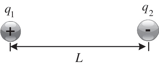

  

  See Exercise (6)

• (7) Three negative point charges are placed at the vertices of an isosceles triangle as shown in the opposite figure. Given that $a=10\,\hbox{cm}, \,q_{ 1} =q_{ 3} =-\;2\;\mu \hbox{C},$ and $q_{ 2} =-\;4\,\mu \hbox{C},$ find the magnitude and direction of the electric field at point P (which is midway between $q_{ 1}$ and $q_{ 3}).$ Fig. (20.25).

  Fig. 20.25

  

  See Exercise (7)

• (8) Four charges of equal magnitude are located at the four corners of a square of side $a=0.1\;\hbox{m}.$ Find the magnitude and direction of the electric field at the center P of the square if: (a) all the charges are positive, i.e., $q_{ i} =5 \,\mu \hbox{C},$ where $i=1,2,3,4,$ see top of Fig. 20.26. (b) the charges alternate in sign around the perimeter of the square, i.e., $q_{ 1} =q_{ 3} =5\,\mu \hbox{C}$ and $q_{ 2} =q_{ 4} =- 5\,\mu \hbox{C},$ see middle of Fig. 20.26. (c) the anti-clockwise sequence of the charge signs around the perimeter are plus, plus, minus, and minus, i.e., $q_{ 1} =q_{ 2} =5 \,\mu \hbox{C}$ and $q_{ 3} =q_{ 4} =- 5\,\mu \hbox{C},$ see lower of Fig. 20.26.

Fig. 20.26

See Exercise (8)

$\user2{Section\; 3.\; Electric \; Field\; of\; an \; Electric\; Dipole}$

• (9) Two point charges $q_{ 1} =- 6\;\mu \hbox{C}$ and $q_{ 2} =+ 6\;\mu \hbox{C}$ are placed at two vertices of an equilateral triangle, see Fig. 20.27. If $a=10\,\hbox{cm},$ find the electric field at the third corner.

  Fig. 20.27

  

  See Exercise (9)

• (10) A proton and an electron form an electric dipole and are separated by a distance of $2 a=2\times 10^{-10}\,\hbox{m},$ see Fig. 20.28. (a) Use exact formulas to calculate the electric field along the x-axis at $x=-10\;a, \,x=-2 a, \,x=-a/2, \,x=+ a/2, \,x=+2 a,$ and $x=+10\;a.$ (b) Show that at both points $x=\pm 10\;a,$ the approximate formula given by Eq. 20.13 has a very close percentage difference from the exact value.

  Fig. 20.28

  

  See Exercise (10)

• (11) Rework the calculations of exercise (10) but on the y-axis.

$\user2{Section\;4.\; Electric\; Field\; of\; a\; Continuous\; Charge\; Distribution}$

• (12) A non-conductive rod of length L has a total negative charge $-Q$ that is uniformly distributed along its length, see Fig. 20.29. (a) Find the linear charge density of the rod. (b) Use the coordinates depicted in the figure to prove that the electric field at point P, a distance a from the right end of the rod, has the same form as the one given by Eq. (20.27). (c) When P is very far from the rod, i.e. $a\gg L,$ show that the electric field reduces to the electric field of a point charge (i.e., the rod would look like a point charge). (d) If $L=15\;\hbox{cm}, \,Q=25\;\mu \hbox{C},$ and$a=20\;\hbox{cm},$ find the value of the electric field at P.

  Fig. 20.29

  

  See Exercise (12)

• (13) A non-conductive rod lies along the x-axis with one of its ends located at x = a and the other end located at $\infty ,$ see Fig. 20.30. Starting from the definition of an electric field of a differential element on the rod, find the electric field at the origin if: (a) the rod carries a uniform positive linear charge density $\lambda .$ (b) the rod carries a positive varying linear charge density $^{ }\lambda =\lambda _{\circ} a/x.$

  Fig. 20.30

  

  See Exercise (13)

• (14) A uniformly charged ring of radius 15 cm has a total charge of $50\,\mu \hbox{C}.$ Find the electric field on the central perpendicular axis of the ring at: (a) 0 cm, (b) 1 cm, (c) 10 cm, and (d) 100 cm. (e) What do you observe about the values you just calculated?

• (15) A charged ring of radius $R=0.5\;\hbox{m}$ has a gap $d=0.1\;\hbox{m},$ see Fig. 20.31. Calculate the electric field at its center C if it carries a uniform charge $q=1\;\mu \hbox{C}.$

  Fig. 20.31

  

  See Exercise (15)

• (16) Figure 20.32 shows a non-conductive semicircular arc of radius R that consists of two quarters. The semicircle has a uniform positive total charge Q along its right half, and a uniform negative total charge $-Q$ along its left half. Find the resultant electric field at the center of the semicircle.

  Fig. 20.32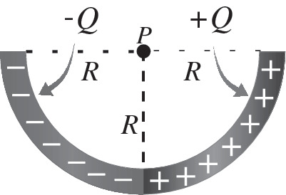

  

  See Exercise (16)

• (17) Two non-conductive semicircular arcs, one of a uniform positive charge +Q and the other of a uniform negative charge $-Q,$ form a circle of radius R, see Fig. 20.33. Find the resultant electric field at the center of the circle, and compare it with the result of exercise 16.

  Fig. 20.33

  

  See Exercise (17)

• (18) If you consider a uniformly charged ring of total charge Q and a fixed radius R (as in Fig. 20.18), then the graph of Fig. 20.34 would map the electric field along the axis of such a ring as a function of z/R. Show that the maximum electric field is $E_{\hbox{max}} =2 k Q/3\sqrt{3} R^{2}$ and occurs at $z=R/\sqrt{2}$

  Fig. 20.34

  

  See Exercise (18)

• (19) An electron is constrained to move along the central axis of a ring of radius R that has a uniform positive charge q, see Fig. 20.35. Show that when the position x of the electron is much less than the radius R $(x\ll R),$ the electrostatic force exerted on the electron can cause it to oscillate through the center of the ring with an angular frequency given by $\omega =\sqrt{k q e/m R^{3}},$ where e and m are the electronic charge and mass, respectively.

  Fig. 20.35

  

  See Exercise (19)

• (20) Two non-conductive rings having the same radius R are arranged with their central axes along a common horizontal line and separated by a distance of 4 R, see Fig. 20.36. Ring 1 has a uniform positive charge $q_{ 1},$ while ring 2 has a uniform positive charge $q_{ 2}.$ Given that the net electric field is zero at point P, which is at a distance R from ring 1 and on the common central axis of the two rings, (a) find the ratio between the two charges. (b) If only the sign of $q_{ 1}$ is reversed, is it possible to have a point on the common axis where the net electric field is zero? If so, where would it be?

  Fig. 20.36

  

  See Exercise (20)

• (21) A disk of radius $R=5\,\hbox{cm}$ has a surface charge density $\sigma =6\;\mu \hbox{C/m}^{2}$ on its surface. Calculate the magnitude of the electric field at points on the central axis of the disk located at: (a) $1\;\hbox{mm},$ (b) $1\;\hbox{cm},$ (c) $10\;\hbox{cm},$ and (d) $100\;\hbox{cm}.$

• (22) A disk of radius R has a charge Q that is uniformly distributed over its surface area. Show that Eq. 20.55 transforms to:

  $$ E=\frac{2 k Q}{R^{2}}\left[{1-\frac{a}{\sqrt{R^{2}+a^{2}}}} \right] $$

  Show that when $a\gg R,$ the electric field approaches that of a point charge formula:

  $$ E\approx k\frac{Q}{a^{2}} \quad (a\gg R) $$

  You may use the binomial expansion $(1 + \delta )^{p}\approx 1+p\delta$ when $\delta \ll 1.$

• (23) Compare the obtained results of exercise 21 to the near-field approximation $E=\sigma /2 \epsilon_{\circ}$ as well as to the point charge approximation $E=k (\pi R^{2}\sigma )/a^{2},$ and find which result(s) of exercise 21 match the two approximations.

• (24) A disk of radius R has a surface charge density $\sigma$ and an electric field of magnitude $E_{\circ} =\sigma /2\epsilon_{\circ}$ at the center of its surface, see Fig. 20.37. At what distance $z$ along the central axis of the disk is the magnitude of the electric field E equal to one-half of $E_{\circ}$?

  Fig. 20.37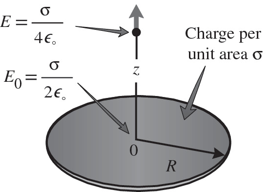

  

  See Exercise (24)

• (25) Find the electric field between two oppositely-charged infinite sheets of charge, each having the same charge magnitude and surface charge density $\sigma ,$ but opposite signs, see Fig. 20.38.

  Fig. 20.38

  

  See Exercise (25)

$\user2{Section\; 5.\; Electric \; Field \; Lines}$

• (26) (a) A negatively charged disk has a uniform charge per unit area. Sketch the electric field lines in a plane perpendicular to the plane of the disk passing through its center. (b) Redo part (a) taking the disk to be positively charged.(c)A negatively charged rod has a uniform charge per unit length. Sketch the electric field lines in the plane of the rod. (d) Three equal positive charges are placed at the corners of an equilateral triangle. Sketch the electric field lines in the plane of the charges. (e) An infinite linear rod has a uniform charge per unit length. Sketch the electric field lines in a plane perpendicular to the rod.

$\user2{Section \; 6 \; Motion \; of \; Charged \; Particles \; in \;a \; Uniform \; Electric \; Field}$

• (27) An electron and a proton are released simultaneously from rest in a uniform electric field of $10^{5}\;\hbox{N/C}.$ Ignore the effect of the fields of the electron and proton on each other. (a) Find the speed and kinetic energy of the electron 50 ns after it has been released. (b) Repeat part (a) for the proton.

• (28) Figure 20.39 shows two oppositely charged parallel plates that are separated by a distance $d=1.5\;\hbox{cm}.$ Each plate has a charge per unit area of magnitude $\sigma =4 \,\mu \hbox{C/m}^{2}.$ An electron is released from rest at t = 0 from the negative plate. (a) Calculate the electric field between the two plates. (b) Ignoring the effect of gravity, find the resultant force exerted on the electron? (c) Find the acceleration of the electron. (d) How long does it take the electron to strike the positive plate? (e) What is the speed and kinetic energy of the electron just before striking the positive plate?

  Fig. 20.39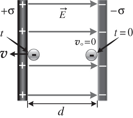

  

  See Exercise (28)

• (29) In exercise 28 assume that the electron is projected from the positive plate toward the negative plate with an initial speed $v_{\circ}$ at time $t=0.$ The electron travels the distance $d=1.5\;\hbox{cm}$ between the two plates and stops temporarily before hitting the negatively charged plate.(a) Find the magnitude and direction of its acceleration. (b) Find the value of the electron’s initial speed. (c) Find the time before the electron stops temporarily.

• (30) Two oppositely charged horizontal plates are separated by a distance $d=1\,\hbox{cm}$ and each has a length $L=3\;\hbox{cm},$ see Fig. 20.40. The electric field between the plates is uniform and has a magnitude $E=10^{2}\,\hbox{ N/m}.$ An electron is projected between the plates with a horizontal initial speed of $v_{\circ} =10^{6}\,\hbox{m/s}$ as shown. Assuming this experiment is conducted in a vacuum, where will the electron strike the upper plate?

  Fig. 20.40

  

  See Exercise (30)

• (31) Repeat exercise 30 when a proton replaces the electron.

• (32) To prevent the electron in exercise 30 from striking the upper plate, its initial horizontal speed is increased to $v_{\circ} =2\times 10^{6}\,\hbox{m/s},$ see Fig. 20.41, and it then strikes a screen at a distance $D=30\;\hbox{cm}.$ (a) What is the acceleration of the electron in the region between the two plates? (b) Find the time when the electron leaves the two plates. (c) What is the vertical position of the electron just before leaving the region between the two plates? (d) Find the electron’s total vertical distance just before hitting the screen.

  Fig. 20.41

  

  See Exercise (32)

• (33) Repeat exercise 32 when a proton replaces the electron.