The Internet in IoT

Abstract

This chapter describes the “Internet” in the “Internet of Things”. It starts with a summary of the well-known Open System Interconnection (OSI) Model Layers. It then describes the TCP/IP Model, which is the basis for the Internet. The TCP/IP protocol has two big advantages in comparison with earlier network protocols: Reliability and flexibility to expand. The TCP/IP protocol was designed for the US Army addressing the reliability requirement (resist breakdowns of communication lines in times of war). The remarkable growth of Internet applications can be attributed to this reliable expandable model.

These keywords were added by machine and not by the authors. This process is experimental and the keywords may be updated as the learning algorithm improves.

Reliable and efficient communication is considered one of the most complex tasks in large-scale networks. Nearly all data networks in use today are based on the Open Systems Interconnection (OSI) standard. The OSI model was introduced by the International Organization for Standardization (ISO), in 1984, to address this complex problem. ISO is a global federation of national standards organizations representing over 100 countries. The model is intended to describe and standardize the main communication functions of any telecommunication or computing system without regard to their underlying internal structure and technology. Its goal is the interoperability of diverse communication systems with standard protocols. The OSI is a conceptual model of how various components communicate in data-based networks . It uses “divide and conquer” concept to virtually break down network communication responsibilities into smaller functions, called layers, so they are easier to learn and develop. With well-defined standard interfaces between layers, OSI model supports modular engineering and multi-vendor interoperability.

2.1 The Open System Interconnection Model

The OSI model consists of seven layers as shown in Fig. 2.1: Physical (layer 1), Data Link (layer 2), Network (layer 3), Transport (layer 4), Session (layer 5), Presentation (layer 6), and Application (layer 7). Each layer provides some well-defined services to the adjacent layer further up or down the stack, although the distinction can become a bit less defined in layers 6 and 7 with some services overlapping the two layers.

Fig. 2.1

OSI layers and data formats

• OSI Layer 7 – Application Layer: Starting from the top, the Application Layer is an abstraction layer that specifies the shared protocols and interface methods used by hosts in a communications network. It is where users interact with the network using higher-level protocols such as DNS (Domain Naming System) , HTTP (Hypertext Transfer Protocol) , Telnet , SSH , FTP (File Transfer Protocol) , TFTP (Trivial File Transfer Protocol) , SNMP (Simple Network Management Protocol) , SMTP (Simple Mail Transfer Protocol) , X Windows , RDP (Remote Desktop Protocol) , etc.

• OSI Layer 6 – Presentation Layer: Underneath the Application Layer is the Presentation Layer . This is where operating system services (e.g., Linux, Unix, Windows, MacOS) reside. The Presentation Layer is responsible for the delivery and formatting of information to the Application Layer for additional processing if required. It ensures that the data can be understood between the sender and receiver. Thus it is tasked with taking care of any issues that might arise where data sent from one system needs to be viewed in a different way by the other system. The Presentation Layer releases the Application Layer of concerns regarding syntactical differences in data representation within the end-user systems. Example of a presentation service would be the conversion of an EBCDIC-coded text computer file to an ASCII-coded file and certain types of encryption such as Secure Sockets Layer (SSL) protocol .

• OSI Layer 5 – Session Layer: Below the Presentation Layer is the Session Layer . The Session Layer deals with the communication to create and manage a session (or multiple sessions) between two network elements (e.g., a session between your computer and the server that your computer is getting information from).

• OSI Layer 4 – Transport Layer: The Transport Layer establishes and manages the end-to-end communication between two end points. The Transport Layer breaks the data, it receives from the Session Layer, into smaller units called Segments . It also ensures reliable data delivery (e.g., error detection and retransmission where applicable). It uses the concept of windowing to decide how much information should be sent at a time between end points. Layer 4 main protocols include Transmission Control Protocol (TCP) and User Datagram Protocol (UDP) . TCP is used for guarantee delivery applications such as FTP and web browsing applications, whereas UDP is used for best effort applications such as IP telephony and video over IP .

• OSI Layer 3 – Network Layer: The Network Layer provides connectivity and path selection (i.e., IP routing ) based on logical addresses (i.e., IP addresses). Hence, routers operate at the Network Layer. The Network Layer breaks up the data it receives from the Transport Layer into packets, which are also known as IP datagrams , which contain source and destination IP address information that is used to forward the datagrams between hosts and across networks.¹ The Network Layer is also responsible for routing of IP datagrams using IP addresses . A routing protocol specifies how routers communicate with each other, exchanging information that enables them to select routes between any two nodes on a computer network. Routing algorithms determine the specific choice of routes. Each router has a priori knowledge only of networks attached to it directly. A routing protocol shares this information first among immediate neighbors and then throughout the network. This way, routers gain knowledge of the topology of the network. The major routing protocol classes in IP networks will be covered in Sect. 2.5. They include interior gateway protocol type 1 , interior gateway protocol type 2, and exterior gateway protocols . The latter are routing protocols used on the Internet for exchanging routing information between autonomous systems.

  It must be noted that while layers 3 and 4 (Network and Transport Layers) are theoretically separated, they are typically closely related to each other in practice. The well-known Internet Protocol name “TCP/IP” comes from the Transport Layer protocol (TCP) and Network Layer protocol (IP).

  Packet switching networks depend upon a connectionless internetwork layer in which a host can send a message without establishing a physical connection with the recipient. In this case, the host simply puts the message onto the network with the destination address and hopes that it arrives. The message data packets may appear in a different order than they were sent in connectionless networks. It is the job of the higher layers, at the destination side, to rearrange out of order packets and deliver them to proper network applications operating at the Application Layer .

• OSI Layer 2 – Data Link Layer: The Data Link Layer defines data formats for final transmission. The Data Link Layer breaks up the data it receives into frames. It deals with delivery of frames between devices on the same LAN using Media Access Control (MAC) Addresses. Frames do not cross the boundaries of a local network. Internetwork routing is addressed by layer 3, allowing data link protocols to focus on local delivery, physical addressing, and media arbitration. In this way, the Data Link Layer is analogous to a neighborhood traffic cop; it endeavors to arbitrate between parties contending for access to a medium, without concern for their ultimate destination. The Data Link Layer typically has error detection (e.g., Cyclical Redundancy Check (CRC)). Typical Data Link Layer devices include switches , bridges, and wireless access points (APs) . Examples of data link protocols are Ethernet for local area networks (multi-node) and the Point-to-Point Protocol (PPP) .

• OSI Layer 1 – Physical Layer: The Physical Layer describes the physical media access and properties. It breaks up the data it receives from the Data Link Layer into bits of zeros and ones (or “off” and “on” signals). The Physical Layer basically defines the electrical or mechanical interface to the physical medium. It consists of the basic networking hardware transmission technologies. It principally deals with wiring and caballing. The Physical Layer defines the ways of transmitting raw bits over a physical link connecting network nodes including copper wires, fiber-optic cables, optical wavelength, and wireless frequencies. The Physical Layer determines how to put a stream of bits from the Data Link Layer on to the pins for a USB printer interface, an optical fiber transmitter, or a radio carrier. The bit stream may be grouped into code words or symbols and converted to a physical signal that is transmitted over a hardware transmission medium . For instance , it uses +5 volts for sending a bit of 1 and 0 volts for a bit of 0 (Table 2.1).

  Table 2.1 Summary of key functions, devices, and protocols of the OSI layers

2.2 End-to-End View of the OSI Model

Figure 2.2 provides an overview of how devices theoretically communicate in the OSI mode. An application (e.g., Microsoft Outlook on a User A’s computer) produces data targeted to another device on the network (e.g., User B’s computer or a server that User A is getting information from). Each layer in the OSI model adds its own information (i.e., headers, trailers) to the front (or both the front and the end) of the data it receives from the layer above it. Such process is called Encapsulation . For instance, the Transport Layer adds a TCP header, the Network Layer adds an IP header, and the Data Link Layer adds Ethernet header and trailer.

Fig. 2.2

Illustration of OSI model

Encapsulated data is transmitted in protocol data units (PDUs) : Segments on the Transport Layer, Packets on the Network Layer, and Frames on the Data Link Layer and Bits on the Physical Layer, as was illustrated in Fig. 2.2. PDUs are passed down through the stack of layers until they can be transmitted over the Physical Layer. The Physical Layer then slices the PDUs into bits and transmits the bits over the physical connection that may be wireless/radio link, fiber-optic, or copper cable. +5 volts are often used to transmit 1 s and 0 volts are used to transmit 0 s on copper cables. The Physical Layer provides the physical connectivity between hosts over which all communication occurs. The Physical Layer is the wire connecting both computers on the network. The OSI model ensures that both users speak the same language on the same layer allowing sending and receiving layers (e.g., networking layers) to virtually communicate. Data passed upward is decapsulated before being passed further up. Such process is called decapsulation . Thus, the Physical Layer chops up the PDUs and transmits the PDUs over the physical connection .

2.3 Transmission Control Protocol/Internet Protocol (TCP/ IP)

TCP/IP (Transmission Control Protocol/Internet Protocol) is a connection-oriented transport protocol suite that sends data as an unstructured stream of bytes. By using sequence numbers and acknowledgment messages, TCP can provide a sending node with delivery information about packets transmitted to a destination node. Where data has been lost in transit from source to destination, TCP can retransmit the data until either a timeout condition is reached or until successful delivery has been achieved. TCP can also recognize duplicate messages and will discard them appropriately. If the sending computer is transmitting too fast for the receiving computer, TCP can employ flow control mechanisms to slow data transfer. TCP can also communicate delivery information to the upper-layer protocols and applications it supports. All these characteristics make TCP an end-to-end reliable transport protocol.

TCP/IP was in the process of development when the OSI standard was published in 1984. The TCP/IP model is not exactly the same as OSI model. OSI is a seven-layered standard, but TCP/IP is a four-layered standard. The OSI model has been very influential in the growth and development of TCP/IP standard, and that is why much of the OSI terminology is applied to TCP/IP.

The TCP/IP Layers along with the relationship to OSI layers are shown in Fig. 2.3. TCP/IP has four main layers: Application Layer, Transport Layer, Internet Layer, and Network Access Layer. Some researchers believe TCP/IP has five layers: Application Layer, Transport Layer, Network Layer, Data Link Layer, and Physical Layer. Conceptually both views are the same with Network Access being equivalent to Data Link Layer and Physical Layer combined.

Fig. 2.3

Relationship between OSI reference model and TCP/IP

2.3.1 TCP/IP Layer 4: Application Layer

As with the OSI model, the Application Layer is the topmost layer of TCP/IP model. It combines the Application, Presentation, and Session Layers of the OSI model. The Application Layer defines TCP/IP application protocols and how host programs interface with Transport Layer services to use the network.

2.3.2 TCP/IP Layer 3: Transport Layer

The Transport Layer is the third layer of the four-layer TCP/IP model. Its main tenacity is to permit devices on the source and destination hosts to carry on a conversation. The Transport Layer defines the level of service and status of the connection used when transporting data. The main protocols included at the Transport Layer are TCP (Transmission Control Protocol) and UDP (User Datagram Protocol) .

2.3.3 TCP/IP Layer 2: Internet Layer

The Internet Layer of the TCP/IP stack packs data into data packets known as IP datagrams , which contain source and destination address information that is used to forward the datagrams between hosts and across networks. The Internet Layer is also responsible for routing of IP datagrams.

The main protocols included at the Internet Layer are IP (Internet Protocol) , ICMP (Internet Control Message Protocol) , ARP (Address Resolution Protocol) , RARP (Reverse Address Resolution Protocol), and IGMP (Internet Group Management Protocol) .

The main TCP/IP Internet Layer (or Networking Layer in OSI) devices are routers. Routers are similar to personal computers with hardware and software components that include CPU, RAM, ROM, flash memory, NVRAM, and interfaces. Given the importance of the router’s role in IoT, we’ll use the next section to describe its main functions .

Router Main Components

There are quite a few types and models of routers. Generally speaking, every router has the same common hardware components as shown in Fig. 2.4. Depending on the model, router’s components may be located in different places inside the router.

Fig. 2.4

Router main components

• 1. CPU (Central Processing Unit) : CPU is an older term for microprocessor, the central unit containing the logic circuitry that preforms the instruction of a router’s program. It is considered as the brain of the router or a computer. CPU is responsible for executing operating system commands including initialization, routing, and switching functions.

• 2. RAM (Random Access Memory) : As with PCs, RAM is a type of computer memory that can be accessed randomly; that is, any byte of memory can be accessed without touching the preceding bytes. RAM is responsible for storing the instructions and data that CPU needs to execute. This read/write memory contains the software and data structures that allow the router to function. RAM is volatile memory, so it loses its content when the router is powered down or restarted. However, the router also contains permanent storage areas such as ROM, flash memory, and NVRAM. RAM is used to store the following:

  • (a) Operating system: The software image (e.g., Cisco’s IOS) is copied into RAM during the boot process.

  • (b) “Running Config” file: This file stores the configuration commands that cisco IOS software is currently using on the router.

  • (c) IP routing tables: Routing tables are used to determine the best path to route packets to destination devices. It’ll be covered in Sect. 2.5.3.

  • (d) ARP cache: ARP cache contains the mapping between IP and MAC addresses. It is used on routers that have LAN interfaces such as Ethernet.

  • (e) Buffer: Packets are temporary stored in a buffer when they are received on congested interface or before they exit an interface .

• 3. ROM (Read-Only Memory): As the name indicates, read-only memory typically refers to hardwired memory where data (stored in ROM) cannot be changed/modified except with a slow and difficult process. Hence, ROM is a form of permanent storage used by the router. It contains code for basic functions to start and maintain the router. ROM contains the ROM monitor, which is used for router disaster recovery functions such as password recovery. ROM is nonvolatile; it maintains the memory contents even when the power is turned off.

• 4. Flash Memory: Flash memory is nonvolatile computer memory that can be electrically stored and erased. Flash is used as permanent storage for the operating system. In most models of Cisco router, Cisco IOS software is permanently stored in flash memory.

• 5. NVRAM (Nonvolatile RAM) : NVRAM is used to store the startup configuration file “startup config,” which is used during system startup to configure the software. This is due to the fact that NVRAM does not lose its content when the power is turned off. In other words, the router’s configuration is not erased when the router is reloaded.

  Recall that all configuration changes are stored in the “running config” file in RAM. Hence, to save the changes in the configuration in case the router is restarted or loses power, the “running config” must be copied to NVRAM, where it is stored as the “startup configuration” file.

  Finally, NVRAM contains the software Configuration Register, a configurable setting in Cisco IOS software that determines which image to use when booting the router.

• 6. Interfaces: Routers are accessed and connected to the external world via the interfaces. There are several types of interfaces . The most common interfaces include:

  • (a) Console (Management) Interface: Console port or interface is the management port which is used by administrators to log on to a router directly (i.e., without using a network connection) via a computer with an RJ-45 or mini-USB connector. This is needed since there is no display device for a router. The console port is typically used for initial setup given the lack of initial network connections such as SSH or HTTPS. A terminal emulator application (e.g., HyperTerminal or PuTTy) is required to be installed on the PC to connect to router. Console port connection is a way to connect to the router when a router cannot be accessed over the network .

  • (b) Auxiliary Interface: Auxiliary port or interface allows a direct, non-network connection to the router, from a remote location. It uses a connector type to which modems can plug into, which allows an administrator from a remote location to access the router like a console port. Auxiliary port is used as a way to dial in to the router for troubleshooting purposes should regular connectivity fail. Unlike the console port, the auxiliary port supports hardware flow control, which ensures that the receiving device receives all data before the sending device transmits more. In cases where the receiving device’s buffers become full, it can pass a message to the sender asking it to temporarily suspend transmission. This makes the auxiliary port capable of handling the higher transmission speeds of a modem.

    Much like the console port, the auxiliary port is also an asynchronous serial port with an RJ-45 interface. Similarly, a rollover cable is also used for connections, using a DB-25 adapter that connects to the modem. Typically, this adapter is labeled “MODEM. ”

  • (c) USB Interface : It is used to add a USB flash drive to a router.

  • (d) Serial Interfaces (Asynchronous and Synchronous) : Configuring the serial interface allows administrators to enable applications such as wide area network (WAN) access, legacy protocol transport, console server, and remote network management.

  • (e) Ethernet Interface : Ethernet is the most common type of connection computers use in a local area network (LAN ). Some vendors categorize Ethernet ports into three areas:

    • (i) Standard/Classical Ethernet (or just Ethernet): Usual speed of Ethernet is 10 Mbps.

    • (ii) Fast Ethernet : Fast Ethernet was introduced in 1995 with a speed of 100Mbps (10x faster than standard Ethernet). It was upgraded by improving the speed and reducing the bit transmission time. In standard Ethernet, a bit is transmitted in 1 second, and in Fast Ethernet it takes 0.01 microseconds for 1 bit to be transmitted. So, 100Mbps means transferring speed of 100 Mbits per second .

    • (iii) Gigabit Ethernet: Gigabit Ethernet was introduced in 1999 with a speed of 1000 Mbps (10x faster than Fast Ethernet and 100x faster than classical Ethernet) and became very popular in 2010. Gigabit Ethernet maximum network limit is 70 km if single-mode fiber is used as a medium. Gigabit Ethernet is deployed in high-capacity backbone network links. In 2000, Apple’s Power Mac G4 and PowerBook G4 were the first mass-produced personal computers featuring the 1000BASE-T connection [2]. It quickly became a built-in feature in many other computers .

      Faster Gigabit Ethernet speeds have been introduced by vendors including 10 Gbps and 100 Gbps, which is supported, for example, by the Cisco Nexus 7700 F3-Series 12-Port 100 Gigabit Ethernet module (Fig. 2.5).

      Fig. 2.5

      

      Example of a router’s rear panel . (Source: Cisco)

Table 2.2 outlines the main functions of each of the router’s components .

Table 2.2 Main functions of the router’s component

2.3.4 TCP/IP Layer 1: Network Access Layer

The Network Access Layer is the first layer of the four-layer TCP/IP model. It combines the Data Link and the Physical Layers of the OSI model. The Network Access Layer defines details of how data is physically sent through the network. This includes how bits are electrically or optically signaled by hardware devices that interface directly with a network medium , such as coaxial cable, optical fiber, radio links, or twisted pair copper wire. The most common protocol included in the Network Access Layer is Ethernet . Ethernet uses Carrier Sense Multiple Access/Collision Detection (CSMA/CD) method to access the media, when Ethernet operates in a shared media. Such Access Method determines how a host will place data on the medium .

2.4 IoT Network Level: Key Performance Characteristics

As we illustrated in Chap. 1, the IoT reference framework consists of four main levels: IoT Device Level (e.g., sensors and actuators), IoT Network Level (e.g., IoT gateways, routers, switches), IoT Application Services Platform Level (the IoT Platform, Chap. 7), and IoT Application Level.

The IoT Network Level is in fact the TCP/IP Layers as shown in Fig. 2.6. It should be noted that we have removed TCP/IP’s Application Layer to prevent overlap with the IoT Application Level.

Fig. 2.6

Mapping of IoT reference framework to TCP/IP Layers

In this section we’ll discuss the most important performance characteristics of IoT network elements. Such features are essential in evaluating and selecting IoT network devices especially IoT gateways, routers, and switches.

IoT Network Level key characteristics may be grouped into three main areas: end-to-end delay, packet loss, and network element throughput. Ideally, engineers want the IoT network to move data between any end points (or source and destination) instantaneously, without any delay or packet loss. However, the physical laws in the Internet constrain the amount of packets that can be transferred between end points per second (known as throughput), present various types of delays to transfer packets from source to destination, and can indeed lose packets.

2.4.1 End-to-End Delay

End-to-end delay across the IoT network is perhaps the most essential performance characteristic for real-time applications especially in wide area networks (WAN) that connect multiple geographies. It may be defined as the amount of time (typically in fractions of seconds) for a packet to travel across the network from source to destination (e.g., from host A to host B as shown in Fig. 2.7). Measuring the end-to-end delay is not a trivial task as it typically varies from one instance to another. Engineers, therefore, are required to measure the delay over a specific period of time and report the average delay, the maximum delay, and the delay variation during such period (known as jitter ). Hence, jitter is defined as the variation in the delay of received packets between a pair of end points.

Fig. 2.7

End-to-end delay from host A to host B with illustration at router A

In general, there are several contributors to delay across the network (as shown in Fig. 2.7). The main ones are the following:

• Processing delay : which is defined as the time a router takes to process the packet header and determine where to forward the packet. It may also include the time needed to check for bit-level errors in the packet (typically in the order of microseconds).

• Queuing delay : which is defined as the time the packet spends in router queues as it awaits to be transmitted onto the outgoing link. Clearly Queuing delay depends on the number of earlier-arriving packets in the same queue (typically in the order of microseconds to milliseconds).

• Transmission delay : which is defined as the time it takes to push the packet’s bits onto the link. Transmission delay of packet of length L bits is defined L/R where R is the transmission rate of a link between two devices. For example, for a packet of length 1000 bits and a link of speed of 100 Mbps, the delay is 0.01 milliseconds. (Transmission delay is typically in the order of microseconds to milliseconds. )

• Propagation delay : which is defined as the time for a bit (of the packet) to propagate from the beginning of a link (once it leaves the source router) to reach its destination router. Hence, Propagation delay on a given link depends on the physical medium of the link itself (e.g., twisted pair copper, fiber, coaxial cable) and is equal to the distance of the link (between two routers) divided by the propagation speed (e.g., speed of light). (Propagation delay is typically in the order of milliseconds). It should be noted that unlike Transmission delay (i.e., the amount of time required to push a packet out), Propagation delay is independent of the packet length.

Hence, the total delay (d _Total), between two end points, is the sum of the Processing delay (d _Process), the Queuing delay (d _Queue), the Transmission delay (d _Trans), and the Propagation delay (d _Prop) across utilized network elements in the path, i.e.,

$$ {D}_{\mathrm{Total}}={d}_{\mathrm{Process}}+{d}_{\mathrm{Queue}}+{d}_{\mathrm{Trans}}+{d}_{\mathrm{Prop}} $$

End-to-end delay is typically measured using Traceroute utility (available on many modern operating systems) as well as vendor-specific tools (e.g., Cisco’s IP SLA (service-level agreement) that continuously collects data about delay, jitter, response time, and packet loss). What is the other utility/command that returns only the final roundtrip times from the destination point (see Problem 27)?

A Traceroute utility’s output displays the route taken between two end systems, listing all the intermediate routers across the network. For each intermediate router, the utility also shows the roundtrip delay (from source to the intermediate router) and time to live (a mechanism that limits the lifetime of the traceroutes packet). Other advantageous of Traceroute utility includes troubleshooting (showing the network administrator bottlenecks and why connections to a destination server are poor) and connectivity (showing how systems are connected to each other and how a service provider connects to the Internet).

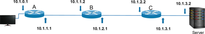
Figure 2.8 shows a simple example of Traceroute utility to trace a path from a client (connected to router A) to the server. In this case, the client enters the command “traceroute 10.1.3.2.” Traceroute utility will display four roundtrip delays, based on three different test packets, sent from the client’s computer to router A, client’s computer to router B, client’s computer to router C, and finally client’s computer to the server .

Fig. 2.8

Traceroute example

The output shows that the roundtrip delay from the client’s computer to router A (ingress port) is 1 msec for the first test packet, 2 msec for the second test packet, and 1 msec for the third and final test. It should be noted that “three test packets” is a typical default value in Traceroute tool and can be adjusted as needed. Also, other parameters may be reported by the tool (e.g., time to live (TTL)) depending on the user’s tool configurations .

Verse

Verse A# trceroute 10.1.3.2 Type escape sequence to abort. Tracing the route to 10.1.3.2 1 10.1.0.2 1 msec, 2 msec, 1 msec 2 10.1.1.2 13 msec, 14 msec, 15 msec 3 10.1.2.2 26 msec, 31 mesec, 29 msec 4 10.1.3.2 41 msec, 43 mesec, 44 msec

2.4.2 Packet Loss

Packet loss occurs when at least one packet of data travelling across a network fails to reach its destination. In general, packets are dropped and consequently lost when the network is congested (i.e., one of the network elements is already operating at full capacity and cannot keep up with arriving packets). This is due to the fact that both queues and links have finite capacities. Hence, a main reason for packet loss is link or queue congestion (i.e., a link between two devices, and its associated queues, is fully occupied when data arrives). Another reason for packet loss is router performance (i.e., links and queues have adequate capacity, but the device’s CPU or memory is fully utilized and not able to process additional traffic). Less common reasons include faulty software deployed on the network device itself or faulty cables .

It should be noted that packet loss may not be as bad as it first seems. Many applications are able to gracefully handle it without impacting the end user, i.e., the application realizes that a packet was lost, adjusts the transfer speed, and requests data retransmission. This works well for file transfer and emails. However, it does not work well for real-time applications such as video conferencing and voice over IP .

2.4.3 Throughput

Throughput may be defined as the maximum amount of data moved successfully between two end points in a given amount of time. Related measures include the link and device speed (how fast a link or a device can process the information) and response time (the amount of time to receive a response once the request is sent).

Throughput is one of the key performance measures for network and computing devices and is typically measured in bits per second (bps) or gigabits per second (Gbps) at least for larger network devices. The system throughput is typically calculated by aggregating all throughputs across end points in a network (i.e., sum of successful data delivered to all destination terminals in a given amount of time).

The simplest way to show how throughput is calculated is through examples. Assume host A is sending a data file to host B through three routers and the speed (e.g., maximum bandwidth) of link i is R_i as shown in Fig. 2.9. Also assume that each router speed (processing power) is higher than the speed of any link and no other host is sending data. In this example, the throughput is

Fig. 2.9

Throughput for a file transfer from host A to host B with a single route

$$min\mathrm{Inner}\mathrm{space}\left(0\mathrm{x}\mathrm{E}\mathrm{F}07\right)\left({\mathrm{R}}_1,{\mathrm{R}}_2,{\mathrm{R}}_3\mathrm{Inner}\mathrm{space}\left(0\mathrm{x}\mathrm{E}\mathrm{F}07\right)\mathrm{and}\mathrm{Inner}\mathrm{space}\left(0\mathrm{x}\mathrm{E}\mathrm{F}07\right){\mathrm{R}}_4\right)\text{.}$$

Thus if R₁ = R₂ = R₃ = 10Mbps and R₄ = 1Mbps, the throughput is 1 Mbps.

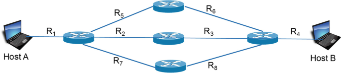
Estimating the throughput is more complicated when multiple paths are allowed in the network. Figure 2.10, for instance, shows that data from host A to host B may take path R₁, R₂, R₃, and R₄ or R₁, R₅, R₆, and R_4.

Fig. 2.10

Throughput for a file transfer from host A to host B with multiple routes

Using the pervious example assumptions (i.e., the speed of each router is higher than the speed of any link and no other host is sending data) and the following new assumptions:

• R₂ = R₃ = R₅ = R₆ = 10 Mbps.

• R₁ = R₄ = 1 Mbps.

• Data is equally divided between the two paths.

The throughput for this example is still 1 Mbps.

Now, if links R₁ and R₄ are upgraded to 100 Mbps, i.e.,

• R₂ = R₃ = R₅ = R₆ = 10 Mbps.

• R₁ = R₄ = 100 Mbps.

• Data is equally divided between the two paths.

Then, the throughput will be 20 Mbps (see Problem 25).

2.5 Internet Protocol Suite

As we mentioned earlier, TCP/IP provides end-to-end connectivity specifying how data should be packetized, addressed, transmitted, routed, and received at the destination. Table 2.3 lists top (partial list) protocols at each layer.

Table 2.3 Examples of Internet protocol suite (partial list)

The objective of this chapter is not to provide an exhaustive list of the TCP/IP protocols but rather to provide a summary of the key protocols that are essential for IoT.

The remainder of this chapter focuses on the main Internet Layer address protocols, namely, IP version 4 and IP version 6. It then describes the main Internet routing protocols, namely, OSPF, EIRGP, and BGP.

2.5.1 IoT Network Level: Addressing

As we mentioned earlier in this chapter, Internet Protocol (IP) provides the main internetwork routing as well as error reporting and fragmentation and reassembly of information units called datagrams for transmission over networks with different maximum data unit sizes. IP addresses are globally unique numbers assigned by the Network Information Center. Globally unique addresses permit IP networks anywhere in the world to communicate with each other. Most of existing networks today use IP version 4 (IPv4). Advanced networks uses IP version 6 (IPv6).

2.5.1.1 IP Version 4

IPv4 addresses are normally expressed in dotted-decimal format , with four numbers separated by periods, such as 192.168.10.10. It consists of 4-octets (32-bit) number that uniquely identifies a specific TCP/IP (or IoT) network and a host (computer, printer, router, IP-enabled sensor, any device requiring a network interface card) within the identified network. Hence, an IPv4 address consists of two main parts: the network address part and the host address part . A subnet mask is used to divide an IP address into these two parts. It is used by the TCP/IP protocol to determine whether a host is on the local subnet or on a remote network.

2.5.1.1.1 IPv4 Subnet Mask

It is important to recall that in TCP/IP (or IoT) networks , the routers that pass packets of data between networks do not know the exact location of a host for which a packet of information is destined. Routers only know what network the host is a member of and use information stored in their route table to determine how to get the packet to the destination host’s network. After the packet is delivered to the destination’s network, the packet is delivered to the appropriate host. For this process to work, an IP address is divided into two parts: network address and host address.

To better understand how IP addresses and subnet masks work, IP addresses should be examined in binary notation. For example, the dotted-decimal IP address 192.168.10.8 is (in binary notation) the 32 bit number 11000000.10101000.00001010.00001000. The decimal numbers separated by periods are the octets converted from binary to decimal notation.

The first part of an IP address is used as a network address and the last part as a host address. If you take the example 192.168.10.8 and divide it into these two parts, you get the following: 192.168.10.0 network address and .8 host address or 192.168.10.0 network address and 0.0.0.8 host address.

In TCP/IP, the parts of the IP address that are used as the network and host addresses are not fixed, so the network and host addresses above cannot be determined unless you have more information. This information is supplied in another 32-bit number called a subnet mask. In the above example, the subnet mask is 255.255.255.0. It is not obvious what this number means unless you know that 255 in binary notation equals 11111111; so, the subnet mask is:

$$ \mathrm{11111111.11111111.11111111.0000000} $$

Lining up the IP address and the subnet mask together, the network and host portions of the address can be separated:

$$ {\displaystyle \begin{array}{l}\mathrm{11000000.10101000.00001010.10001000}--\mathrm{IP}\ \mathrm{address}\ \left(\mathrm{192.168.10.8}\right)\\ {}\mathrm{11111111.11111111.11111111.00000000}--\mathrm{Subnet}\ \mathrm{mask}\ \left(\mathrm{255.255.255.0}\right)\end{array}} $$

The first 24 bits (the number of ones in the subnet mask) are identified as the network address, with the last 8 bits (the number of remaining zeros in the subnet mask) identified as the host address . This gives you the following:

$$ {\displaystyle \begin{array}{l}\mathrm{11000000.10101000.00001010.00000000}--\mathrm{Network}\ \mathrm{address}\ \left(\mathrm{192.168.10.0}\right)\\ {}\mathrm{00000000.00000000.00000000.00001000}--\mathrm{Host}\ \mathrm{address}\ \left(\mathrm{000.000.000.8}\right)\end{array}} $$

2.5.1.1.2 IPv4 Classes

Five classes (A, B, C, D, and E) have been established to identify the network and host parts. All the five classes are identified by the first octet of IP address. Classes A, B, and C are used in actual networks. Class D is reserved for multicasting (data is not destined for a particular host; hence there is no need to extract host address from the IP address). Class E is reserved for experimental purposes.

Figure 2.11 shows IPv4 address formats for classes A, B, and C. Class A networks provide only 8 bits for the network address field and 24 bits for host address. It is intended mainly for use with very large networks with large number of hosts. The first bit of the first octet is always set to 0 (zero). Thus the first octet ranges from 1 to 127, i.e., 00000001–011111111. Class A addresses only include IP starting from 1.x.x.x to 126.x.x.x only. The IP range 127.x.x.x is reserved for loopback IP addresses. The default subnet mask for class A IP address is 255.0.0.0 which implies that class A addressing can have 126 networks (2⁷–2) and 16777214 hosts (2²⁴–2).

Fig. 2.11

IPv4 address formats for classes A, B, and C

Class B networks allocate 16 bits for the network address field and 16 bits for the host address filed. An IP address which belongs to class B has the first two bits in the first octet set to 10, i.e., 10000000 – 10111111 or 128–191 in decimal. Class B IP addresses range from 128.0.x.x to 191.255.x.x. The default subnet mask for class B is 255.255.x.x. Class B has 16384 (2¹⁴) network addresses and 65534 (2¹⁶–2) host addresses.

Class C networks allocate 24 bits for the network address field only 8 bits for the host field. Hence, the number of hosts per network may be a limiting factor. The first octet of Class C IP address has its first 3 bits set to 110, that is: 1110 0000–1110 1111 or 224–239 in decimal.

Class C IP addresses range from 192.0.0.x to 223.255.255.x. The default subnet mask for Class C is 255.255.255.x. Class C gives 2097152 (2²¹) Network addresses and 254 (2⁸–2) Host addresses.

Finally, IP networks may also be divided into smaller units called subnetworks or subnets for short . Subnets provide great flexibility for network administrators. For instance, assume that a network has been assigned a Class A address and all the nodes on the network use a Class A address. Further assume that the dotted-decimal representation of this network’s address is 28.0.0.0. The network administrator can subdivide the network using sub-netting by “borrowing” bits from the host portion of the address and using them as a subnet field .

2.5.1.2 IP Version 6

IPv4 has room for about 4.3 billion addresses, which is not nearly enough for the world’s people, let alone IoT with a forecast of 20 billion devices by 2020. In 1998, the Internet Engineering Task Force (IETF) had formalized the successor protocol: IPv6. IPv6 uses a 128-bit address, allowing 2¹²⁸ or 340 trillion trillion trillion (3.4 × 10³⁸) addresses. This translates to about 667 × 10²¹ (667 sextillion) addresses per square meter in earth. Version 4 and version 6 protocols are not designed to be interoperable, complicating the transition to IPv6. However, several IPv6 transition mechanisms have been devised to permit communication between IPv4 and IPv6 hosts.

IPv6 delivers other benefits in addition to a larger addressing space. For example, permitting hierarchical address allocation techniques that limit the expansion of routing tables simplified and expanded multicast addressing and service delivery optimization. Device mobility, security, and configuration aspects have been considered in the design of IPv6.

• I. IPv6 Addresses Are Broadly Classified Into Three Categories:

  • Unicast addresses : A unicast address acts as an identifier for a single interface. An IPv6 packet sent to a unicast address is delivered to the interface identified by that address.

  • Multicast addresses: A multicast address acts as an identifier for a group/set of interfaces that may belong to different nodes. An IPv6 packet delivered to a multicast address is delivered to the multiple interfaces.

  • Anycast addresses: Anycast addresses act as identifiers for a set of interfaces that may belong to different nodes. An IPv6 packet destined for an anycast address is delivered to one of the interfaces identified by the address.

2.5.2 IPv6 Address Notation

The IPv6 address is 128 bits long. It is divided into blocks of 16 bits. Each 16-bit block is then converted to a 4-digit hexadecimal number, separated by colons. The resulting representation is called colon-hexadecimal . This is in contrast to the 32-bit IPv4 address represented in dotted-decimal format, divided along 8-bit boundaries, and then converted to its decimal equivalent, separated by periods.

• II. IPV6 Example

  • Binary Form

    0111000111011010000000001101001100000000000000000010111100111011

    0000001010101010000000001111111111111110001010001001110001011011

  • 16-Bit Boundaries Form

    0111000111011010 0000000011010011 0000000000000000 0010111100111011

    0000001010101010 0000000011111111 11111110001010001001110001011011

  • 16-Bit Block Hexadecimal and Delimited with Colons Form

    71DA:00D3:0000:2F3B:02AA:00FF:FE28:9C5B.

    i.e., (0111000111011010)₂ = (71DA)₁₆, (0000000011010011)₂ = (D3)₁₆, and so on.

  • Final Form ( 16-Bit Block Hexadecimal and Delimited with Colons Form, Simplified by Removing the Leading Zeros).

    71DA:D3:0:2F3B:2AA:FF:FE28:9C5B

2.5.3 IoT Network Level: Routing

Routers use routing tables to communicate: send and receive packets among themselves. TCP/IP routing specifies that IP packets travel through an internetwork one router hop at a time. Hence, the entire route is not known at the beginning of the journey. Instead, at each stop, the next router hop is determined by matching the destination address within the packet with an entry in the current router’s routing table using internal information.

Before describing the main routing protocols in the Internet today, it is important to introduce a few fundamental definitions.

• Static Routes: Static routes define specific paths that are manually configured between two routers. Static routes must be manually updated when network changes occur. Static routes use should be limited to simple networks with predicted traffic behavior.

• Dynamic Routes: Dynamic routing requires the software in the routing devices to calculate routes. Dynamic routing algorithms adjust to changes in the network and repeatedly select best routes. Internet-based routing protocols are dynamic in nature. Routing tables should be updated automatically to capture changes in the network (e.g., link just went down, link that was down is no up, link speed update ).

• Autonomous System (AS): It is a network or a collection of networks that are managed by a single entity or organization (e.g., Department Network). An AS may have multiple subnetworks with combined routing logic and common routing policies. Routers used for information exchange within AS are called interior routers . They use a variety of interior routing protocols such as OSPF and EIGRP. Routers that move information between autonomous systems are called exterior routers, and they use the exterior gateway protocol such as Border Gateway Protocol (BGP) . Interior routing protocols are used to update the routing tables of routers within an AS. In contrast, exterior routing protocols are used to update the routing tables of routers that belong to different AS. Figure 2.12 shows an illustration of two autonomous systems connected by BGP external routing protocol.

  Fig. 2.12

  

  Example of autonomous systems

• Routing Table: Routing tables basically consist of destination address and next hop pairs. Figure 2.13 shows an example of a typical Cisco router routing table using the command “show ip route”. It lists the set of comprehensive codes including various routing schemes. Figure 2.13 also shows that the first entry is interpreted as meaning “to get to network 29.1.0.0 (subnet 1 on network 24), the next stop is the node at address 51.29.23.12.” We’ll refer to this figure as we introduce various routing schemes .

  Fig. 2.13

  

  Example of a routing table

• Distance Vector Routing: A vector in distance vector routing contains both distance and direction to determine the path to remote networks using hop count as the metric. A hop count is defined as the number of hops to destination router or network (e.g., if there two routers between a source router and destination router, the number of hops will be three). All neighbor routers will send information about their connectivity to their neighbors indicating how far other routers are from them. Hence, in distance vector routing, all routers exchange information only with their neighbors (not with all routers). One of the weaknesses of distance vector protocols is convergence time, which is the time it takes for routing information changes to propagate through all the topology .

• Link-State Routing: Contrast to distance vector, link-state routing requires all routers to know about the paths reachable by all other routers in the network. In this case, link-state data is flooded to the entire router in AS. Link-state routing requires more memory and processor power than distance vector routing. Also, link-state routing can degrade the network performance during the initial discovery process, as it requires flooding the entire network with link-state advertisements (LSAs) .

2.5.3.1 Interior Routing Protocols

Interior gateway protocols (IGPs) operate within the confines of autonomous systems . We will next describe only the key protocols that are currently popular in TCP/IP networks. For additional information, the reader is encouraged to peruse the references at the end of the chapter.

• A. Routing Information Protocol ( RIP) : RIP is perhaps the oldest interior distance vector protocol. It was developed by Xerox Corporation in the early 1980s. It uses hop count (maximum is 15) and maintains times to detect failed links. RIP has a few serious shortcomings: it ignores differences in line speed, line utilization, and other metrics. More significantly, RIP is very slow to converge for larger networks, consumes too much bandwidth to update the routing tables, and can take a long time to detect routing loops .

• B. Enhanced Interior Gateway Routing Protocol (EIGRP) : Cisco was the first company to solve RIP’s limitations by introducing the interior gateway routing protocol (IGRP) first in the mid-1980s. IGRP allows the use of bandwidth and delay metrics to determine the best path. It also converges faster than RIP by preventing sharing hop counts and avoiding potential routing loops caused by disagreement over the next routing hop to be taken.

  Cisco then enhanced IGRP to handle larger networks. The enhanced IGRP (EIGRP) combines the ease of use of traditional distance vector routing protocols with the fast rerouting capabilities of the newer link-state routing protocols. It consumes significantly less bandwidth than IGRP because it is able to limit the exchange of routing information to include only the changed information.

• C. Open Shortest Path First (OSPF): Open Shortest Path First (OSPF) was developed by the Internet Engineering Task Force (IETF) in RFC-2328 as a replacement for RIP. OSPF is based on work started by John McQuillan in the late 1970s and continued by Radia Perlman and Digital Equipment Corporation in the mid-1980s. OSPF is widely used as the Interior Router protocol in TCP/IP networks. OSPF is a link-state protocol , so routers inside an AS only broadcast their link-states to all the other routers. It uses configurable least cost parameters including delay, data rate/link speed, cost, and other parameters. Each router maintains a database topology of the AS to which it belongs. In OSPF every router calculates the least cost path to all destination networks using Dijkstra’s algorithm . Only the next hop to the destination is stored in the routing table.

  OSPF maintains three separate tables: neighbor table, link-state database table, and routing table.

  • Neighbor Table : Neighbor table uses the so-called Hello Protocol to build neighbor relationship. The relationship is used to exchange information with all neighbors for the purpose of building the link-state DB table. When a new router joins the network, it sends a “Hello” message periodically to all neighbors (typically every few seconds). All neighbors will also send Hello messages. The messages maintain the state of the neighbor tables .

  • Link-State DB Table : Once the neighbor tables are built, link-state advertisements (LSAs) will be sent out to all neighbors. LSAs are packets that contain information about networks that are directly connected to the router that is advertising. Neighboring routers will receive the LSAs and add the information to the link-state DB. They then increment the sequence number and forward LSAs to their neighbors. Hence, LSAs are prorogated from routers to all the neighbors with advertised information about all networks connected to them. This is considered the key to dynamical routing .

  • Routing Table : Once the link-state DB tables are built, Dijkstra’s algorithm (sometimes called the Shortest Path First Algorithm ) is used to build the routing tables .

• D. Integrated Intermediate System to Intermediate System (IS-IS) : Integrated IS-IS is similar in many ways to OSPF. It can operate over a variety of subnetworks, including broadcast LANs, WANs, and point-to-point links. IS-IS was also developed by IETF as an Internet Standard in RFC 1142.

2.5.3.2 Exterior Routing Protocols

Exterior Routing Protocols provide routing between autonomous systems. The two most popular Exterior Routing Protocols in the TCP/IP are EGP and BGP.

• A. Exterior Gateway Protocol ( EGP) : EGP was the first exterior routing protocol that provided dynamic connectivity between autonomous systems. It assumes that all autonomous systems are connected in a tree topology. This assumption is no longer true and made EGP obsolete.

• B. Border Gateway Protocol ( BGP) : BGP is considered the most important and widespread exterior routing protocol. Like EGP, BGP provides dynamic connectivity between autonomous systems acting as the Internet core routers. BGP was designed to prevent routing loops in arbitrary topologies by preventing routers from importing any routes that contain themselves in the autonomous system’s path. BGP also allows policy-based route selection based on weight (set locally on the router), local preference (indicates which route has local preference and BGP selects the one with the highest preference), network or aggregate (chooses the path that was originated locally via an aggregate or a network), and shortest AS Path (used by BGP only in case it detects two similar paths with nearly the same local preference, weight and locally originated or aggregate addresses) just to name a few.

  BGP’s routing table contains a list of known routers, the addresses they can reach, and a cost metric associated with the path to each router so that the best available route is chosen. BGP is a layer 4 protocol that sits on top of TCP. It is simpler than OSPF, because it doesn’t have to worry about functions that TCP addresses. The latest revision of BGP , BGP4 (based on RFC4271), was designed to handle the scaling problems of the growing Internet .

2.6 Summary

This chapter focused on the “Internet” in the “Internet of Things.” It started with an overview of the well-known Open System Interconnection Model Seven Layers along with the top devices and protocols. It showed how each layer divides the data it receives from end-user applications or from layer above it into protocol data units (PDUs) and then adds additional information to each PDU for tracking. This processed is called the Encapsulation . Examples of PDUs include Segments on the Transport Layer, Packets on the Network Layer, and Frames on the Data Link Layer. PDUs are passed down through the stack of layers until they can be transmitted over the Physical Layer. The OSI model ensures that both users speak the same language on the same layer allowing sending and receiving layers to virtually communicate. Data passed upward is decapsulated, with the decapsulation process, before being passed further up to the destination server, user, or application.

Next, it described the TCP/IP model which is the basis for the Internet. The TCP/IP protocol has two big advantages in comparison with earlier network protocols: reliability and flexibility to expand. In fact, the TCP/IP protocol was designed for the US Army addressing the reliability requirement (resist breakdowns of communication lines in times of war). The remarkable growth of Internet applications can be attributed to its fixable expandability model.

The chapter then introduced the key IoT Network Level characteristics that included end-to-end delay, packet loss, and network element throughput. Such characteristics are vital for network design and vendor selection. The chapter next compared IP version 4 with IP version 6. It showed the limitation of IPv4, especially for the expected 50 billion devices for IoT. IPv4 has room for about 4.3 billion addresses, whereas IPv6, with a 128-bit address, has room for 2¹²⁸ or 340 trillion trillion trillion (3.4 × 10³⁸) addresses. Finally detailed description of IoT Network Level routing was described and compared with classical routing protocols. It was mentioned that routing tables are used in routers to send and receive packets. Another key feature of TCP/IP routing is the fact that that IP packets travel through an internetwork one router hop at a time an thus the entire route is not known at the beginning of the journey.

Problems and Exercises

• 1. Ethernet and Point-to-Point Protocol (PPP) are two examples of data link protocols listed in this chapter. Name two other data link protocols.

• 2. Provide an example of Session Layer protocol.

• 3. In a table format, compare the bandwidth, distance, interference rating, cost and security of (1) twisted pair, (2) coaxial cabling, and (3) fiber optical cabling.

• 4. A. What are the main components of a router? B. Which element is considered the most essential? C. Why?

• 5. What is the main function of NVRAM? Why is such function important to operate a router?

• 6. How do network administrators guarantee that changes in the configuration are not lost in case the router is restarted or loses power?

• 7. What is a disaster recovery function in a router? Which router’s sub-component contains such function?

• 8. Many argue that routers are special computers but built to handle internetwork traffic. List three main differences between routers and personal computers.

• 9. There are no input devices for router like a monitor, a keyboard, or a mouse. How does a network administrator communicate with the router? List all possible scenarios. What are the main differences between such interfaces?

• 10. How many IPv4 addresses are available? Justify your answer.

• 11. What is the ratio of the number of addresses in IPv6 compared to IPv4?

• 12. IPv6 uses a 128-bit address, allowing 2¹²⁸ addresses. In decimal, how many IPv6 addresses exist? How many IPv6 addresses will each human have? Why do we need billions of addresses for each human being?

• 13. How many IPv6 address will be available on each square meter of earth?

• 14. What are the major differences between interior and exterior routing protocols?

• 15. What is distance vector protocol? Why is it called a vector? Where is it used?

• 16. When would you use static routing and when would use dynamic routing? Why?

• 17. Most IP networks use dynamic routing to communicate between routers but may have one or two static routes. Why would you use static routes?

• 18. We have mentioned that in TCP/IP networks, the entire route is not known at the beginning of the journey. Instead, at each stop, the next router hop is determined by matching the destination address within the packet with an entry in the current router’s routing table using internal information. IP does not provide for error reporting back to the source when routing anomalies occur.

  • A. Which Internet Protocol provides error reporting?

  • B. List two other tasks that this protocol provides?

• 19. Why is EGP considered to be obsolete for the current Internet?

• 20. In a table, compare the speed and distance Standard Ethernet, Fast Ethernet, and Giga Ethernet. Why is Ethernet connection limited to 100 meters?

• 21. Why the Internet does require both TCP and IP protocols?

• 22. Are IPv4 and IPv6 protocols designed to be interoperable? How would an enterprise transition from IPv4 to IPv6?

• 23. What are the four different reasons for packet loss? List remediation for each reason.

• 24. List two factors that can affect throughput of a communication system.

• 25. Figure 2.10 (in Section 2.4.3) stated the throughput between host A and host B is 20 mbps with the assumptions:

  • R₂ = R₃ = R₅ = R₆ = 10Mbps.

  • R₁ = R₄ = 100Mbps.

  • Data is equally divided between the two paths.

  How did the authors arrive at 20 Mbps?

• 26. Assuming host A is transferring a large file to host B. What is the throughput between host A and host B for the network shown below?

  

  • A. Assumptions:

    • The speed of each router is higher than the speed of any link in the network.

    • No other host is sending data.

    • R₂ = R₃ = R₅ = R₆ = R₇ = R₈ = 10Mbps.

    • R₁ = R₄ = 1 Mbps.

    • Data is equally divided between the three paths.

  • B. Assumptions:

    • The speed of each router is higher than the speed of any link in the network.

    • No other host is sending data.

    • R2 = R3 = R5 = R6 = R7 = R8 = 10Mbps.

    • R1 = R4 = 100 Mbps.

    • Data is equally divided between the three paths.

  • C. Assumptions:

    • The speed of each router is 1 Mbps.

    • No other host is sending data.

    • R2 = R3 = R5 = R6 = R7 = R8 = 10Mbps.

    • R1 = R4 = 100 Mbps.

    • Data is equally divided between the three paths.

• 27. What is Traceroute? What does it typically report? What are the main advantageous of trace route? What is the main difference between Traceroute and Ping?

• 28. For the network shown below, assume the network administer is interested in measuring the end-to-end delay from router A to the server.

  • A. What is the Traceroute command? Hence, Traceroute command is sent from router A directly (i.e., via the shown connected terminal).

  • B. Which device will send their delays?

  

• 29. What is time to live command? Why is it needed?

References

W. Odom, CCNA Routing and Switching 200–120 Official Cert Guide Library Book, ISBN: 978–1587143878, May 2013
P. Browning, F. Tafa, D. Gheorghe, D. Barinic, Cisco CCNA in 60 Days, ISBN: 0956989292, March 2014
G. Heap, L. Maynes, CCNA Piratical Studies Book (Cisco Press, April 2002)
Information IT Online Library.: http://www.informit.com/library/content.aspx?b=CCNA_Practical_Studies&seqNum=12
Inter NICFootnote
InterNIC is a registered service mark of the US Department of Commerce. It is licensed to the Internet Corporation for Assigned Names and Numbers, which operates this website.
—Public Information Regarding Internet Domain Name Registration Services, Online: http://www.internic.netUnderstanding TCP/IP addressing and subnetting basics, Online: https://support.microsoft.com/en-us/kb/164015
Tutorials Point, “IPv4 – Address Classes”, Online: http://www.tutorialspoint.com/ipv4/ipv4_address_classes.htm
Google IPv6, “What if the Internet ran out of room? In fact, it's already happening”, Online: http://www.google.com/intl/en/ipv6/
Wikipedia, “Internet Protocol version 6 (IPv6):, Online: https://en.wikipedia.org/wiki/IPv6
IPv6 Addresses, Microsoft Windows Mobile 6.5, April 8, 2010, Online: https://msdn.microsoft.com/en-us/library/aa921042.aspx
Binary to Hexadecimal Convert, Online: http://www.binaryhexconverter.com/binary-to-hex-converter
Technology White Paper, Cisco Systems online: http://www.cisco.com/c/en/us/tech/ip/ip-routing/tech-white-papers-list.html
M. Caeser, J. Rexford, “BGP routing policies in ISP networks”, Online: https://www.cs.princeton.edu/~jrex/papers/policies.pdf
A. Shaikh, A.M. Goyal, A. Greenberg, R. Rajan, An OSPF topology server: Design and evaluation. IEEE J. Sel. Areas Commun 20(4) (2002)
Y. Yang, H. Xie, H. Wang, A. Silberschatz, Y. Liu, L. Li, A. Krishnamurthy, On route selection for interdomain traffic engineering. IEEE Netw. Mag. Spec. Issue Interdomain Rout (2005)
N. Feamster, J. Winick, J. Rexford, “A model of BGP routing for network engineering,” in Proc. ACM SIGMETRICS, June 2004
N. Feamster, H. Balakrishnan, Detecting BGP configuration faults with static analysis, in Proc. Networked Systems Design and Implementation, (2005)
Apple History / Power Macintosh Gigabit Ethernet, Online: http://www.apple-history.com/g4giga. Retrieved November 5, 2007
Author information
Authors and Affiliations