Smoothness in Some Varieties with Dihedral Symmetry and the DFT Matrix

Abstract

We study the smoothness question for some families of real and complex varieties with cyclic or dihedral symmetry. This question is related to deep properties of the Vandermonde matrix on the roots of unity, also known as the Discrete Fourier Transform matrix. We present some partial results on these questions.

Para Antonio Campillo, en sus 65 años.

1 Introduction

For many years I have studied with different collaborators the topology of transverse intersections of quadrics in $\mathbb {R}^n$. I will try to give a synthesis of the main results.

Starting from the most general ones, we have a characterization of the compact smooth manifolds which are transverse intersections of quadrics or transverse intersections of ellipsoids [9]. More specific intersections that are sometimes easier to describe completely are the transverse intersections of centered ellipsoids

$$\displaystyle \begin{aligned} \begin{array}{rcl}&\displaystyle &\displaystyle Q_i(x)=0,\,\,\, i=1,\dotsc,m\\ &\displaystyle &\displaystyle \qquad \quad \varSigma_{i=1}^n x_i^2=1 \end{array} \end{aligned} $$

(where the Q _i are quadratic forms) or of coaxial ellipsoids, meaning that the quadratic forms are simultaneously diagonalizable:

$$\displaystyle \begin{aligned} \begin{array}{rcl} &\displaystyle &\displaystyle \varSigma_{i=1}^n A_i x_i^2=0\\ &\displaystyle &\displaystyle \,\varSigma_{i=1}^n x_i^2=1 \end{array} \end{aligned} $$

(where $A_i \in \mathbb {R}^m$).

These are relatively easier to study because they have more symmetry: if Z is the previous intersection, changing the sign of x _i leaves invariant Z so there is an action of $\mathbb {Z}_2^n$ on them with quotient $Z\cap \mathbb {R}_+^n$ which is homeomorphic to the convex polyope P:

$$\displaystyle \begin{aligned}\varSigma_{i=1}^n A_i r_i=0\end{aligned}$$

$$\displaystyle \begin{aligned}\varSigma_{i=1}^n r _i=1\end{aligned}$$

$$\displaystyle \begin{aligned}r_i\ge 0,\,\,\, i=1,\dotsc, n\end{aligned}$$

One can recover Z topologically from P by reflecting it in all coordinate hyperplanes x _i = 0. So the convex polytope P and the configuration of coefficients are two combinatorial objects (called Gale dual) that contain all the information about Z. Furthermore, any polytope can be realized as the polytope P of such an intersection. When the intersection is transverse the polytope is of a special type called simple. This already suggests that a complete description of the topological types is close to the complete classification of the simple polytopes, a goal that looks out of reach.

Nevertheless, we have been able along the years to describe topologically large families of them:

• (A) For m = 2 we have a complete description of all the transversal intersections, including the non-diagonal ones [11].

  For the diagonal ones the configurations are collections of points in the plane, where the basic ones are the vertices of a regular polygon of n sides. So we can write their equations in terms of roots of unity:

  $$\displaystyle \begin{aligned}\varSigma_{i=1}^n \rho^i x_i^2=0\end{aligned}$$
  $$\displaystyle \begin{aligned}\varSigma_{i=1}^n x_i^2=1\end{aligned}$$

  where ρ = e ^2πi∕n.

  The rest of the objects are constructed by taking each of the coefficients with a multiplicity.

  The first step for the topological description of these basic objects is to decide their smoothness. This follows very easily from the general criterion (see Sect. 5): they are smooth if, and only if, n is odd.

  The second step is to describe the topology for all smooth cases and the proof (which includes all the generic non-diagonal cases) is quite long [11, 15, 16]. For the basic configurations it is a connected sum of n copies of S ^(n−3)∕2 × S ^(n−3)∕2; for the configurations with multiplicity it can be a triple product of spheres or a connected sum of spheres of different dimensions.

• (B) For m = n − 3 we get surfaces by realizing the n-gon as the polytope of an intersection. These were first constructed by Hirzebruch as an unpublished side result to [13]. The connected ones have genus g = 2ⁿ⁻³(n − 4) + 1. Other genera can be realized as transverse intersections of centered, non-coaxial ellipsoids [10].

• (C) For m > 2, the generalization of the basic examples in (A) are all those intersections which are connected up to the middle dimension and which are constructed from the dual of a special type of polytope (called neighbourly). When taken with multiplicities they form a large subset of the possible cases and when the dimension is as least 5, it can be proved that they all are connected sums of products of spheres of different dimensions [8].

• (D) Simple operations with the polytopes, such as products or truncation of a vertex or another face give rise to many new examples with known topology [8].

More recently, explicit equations were constructed in [6] of the equations for the surfaces in (B) such that the associated polygon is regular. One form of these equations is as follows:

$$\displaystyle \begin{aligned}\varSigma_{i=1}^n \rho^{ki} x_i^2=0,\,\,\,k=2,\dots,[n/2]\end{aligned}$$

$$\displaystyle \begin{aligned}\varSigma_{i=1}^n x_i^2=1\end{aligned}$$

The homogeneous equations are of the same type as those in the basic example in (A), but different roots of unity are used in each equation, including powers of ρ from 2 to [n∕2]. So the equations of this example and those of the basic example in (A) are complementary within the natural range 1, …, [n∕2] (observe that higher powers up to n − 1 would give the conjugates of equations already considered and the equation with the n-th power would contradict that of the sphere). Observe that in both cases the configuration of coefficients, the variety and the polytope all have dihedral symmetry.¹

Moreover, there is a strange duality between the examples: surprisingly, the configuration of the coefficients of the first one (the n-gon) coincides with the polytope of the second and viceversa: it turns out that the polytope of the first one coincides combinatorially with the configuration of the coefficients of the second one! However, there is an asymmetry: the second variety is always smooth, while the first one is smooth for n odd only.

A natural generalization in immediate: take K ⊂ [1, …, [n∕2]] and Z(K) be the variety.

$$\displaystyle \begin{aligned}\varSigma_{i=1}^n \rho^{ki} x_i^2=0,\,\,\,k\in K\end{aligned}$$

$$\displaystyle \begin{aligned}\varSigma_{i=1}^n x_i^2=1\end{aligned}$$

The matrix of coefficients consists of rows of the Vandermonde matrix V _n = (ρ ^ij), the n × n Vandermonde matrix evaluated on the n-th roots of unity, also known as the Discrete Fourier Transform (DFT) matrix.

In many particular examples one can check that the same type of duality holds between the combinatorial objects associated to Z(K) and those of the complementary Z(K ^c), while the smoothness of one of them seems to be related to a different regularity property of the other.

This is an interesting phenomenon that is worth understanding. Furthermore, together with the examples obtained by including multiplicities on the basic ones, this is an interesting new family of intersections of ellipsoids that contains and connects the families (A) and (B) and whose topological description could increase our knowledge about this subject.

But this family turns out to be much more difficult to study than the previous ones: just the first step (deciding which are the smooth cases, which in the previous families was easily solved) happens to be an extremely difficult problem in number theory involving the minors of V _n. We have up to now only partial information about this question. The subsequent steps (understanding the precise nature of the observed duality and describing the topology of the smooth examples) look also like two extremely difficult tasks.

The analogous family of projective algebraic varieties with cyclic or dihedral symmetry

$$\displaystyle \begin{aligned}\varSigma_{i=1}^n \rho^{ki} z_i^d=0,\,\,\,k\in K,\,\, d>1,\end{aligned}$$

where K is a subset of [1, …, n] of cardinality m, is an interesting first step for the understanding the above questions. In this family, the relation between the smoothness of the family and the minors of V _n is simpler: smoothness is equivalent to the property that for the m × m matrix of coefficients of the equations, all m × m minors are non zero. This property is relatively simpler from both the theoretical and the computational point of view than the corresponding property in the real case. Furthermore, the duality in this case between complementary examples holds neatly: an example is smooth if, and only if, the complementary one is smooth.

This family is not only a toy example for the understanding of the real case, but it has life of its own: the simpler results about their smoothness already give examples of smooth intersections of hypersurfaces with cyclic or dihedral symmetry that extend to other smooth intersections of hypersurfaces diffeomorphic to them, and in some cases one obtains towers of such varieties all with the same symmetries. Also, the question of their smoothness is connected to some problems of interest in some engineering areas, such as signal recognition or self-correcting codes.

In this article we present the known results about the minors V _n and show how the simplest ones give interesting examples, including towers of them. We also include a conjecture about the topology of the intersections of real quadrics in one of these towers. We leave for another article the exploration of other more elaborate results.

Sections 2 and 3 describe the known results about minors of V _n including some proofs. Section 4 contains some implications of the above to the intersections of complex hypersurfaces while Sect. 5 describes those implications for the intersections of real ellipsoids, including a conjecture about the topology of some towers of them.

Recently we discovered, looking through the literature citing Tao [21] and its sequels, some papers about signal recognition dealing with the same type of problems but under a different name: matrices we call hyperbolic are known in this field as full spark matrices.

In particular, in [1] there are some results about the case g = 1 of our Theorem 4. We also learned there about [2], where a version of our Theorem 2 is proved. In a subsequent article we will describe the relations between those results and ours.

2 Jacobi Formula for the Co-rank

In this section A is a non singular n × n matrix with entries in a field and B = A ⁻¹.

Let I, J be subsets of [1, …, n] and I ^c, J ^c their complements.

We denote by M[I, J] the submatrix of a matrix M consisting of the entries M _ij with i ∈ I and j ∈ J. When M is divided into blocks, we will denote them by

$$\displaystyle \begin{aligned} M=\begin{pmatrix} M_{11} & M_{12} \\ M_{21} & M_{22} \end{pmatrix} \end{aligned}$$

Theorem 1

Assume I and J have the same cardinality. Then

• (i) Determinant Jacobi formula:

  $$\displaystyle \begin{aligned} \big\vert A \big\vert\; \big\vert B[J^c,I^c] \big\vert= \pm \big\vert A[I,J] \big\vert \end{aligned}$$

• (ii) Co-rank formula: The co-rank of the square matrix A[I, J] is equal to the co-rank of the complementary submatrix B[J ^c, I ^c] of the inverse matrix B. In particular, if A[I, J] is invertible then so is B[J ^c, I ^c].

Proof

For both parts, we follow the last proof of (ii) in [18]. A geometric proof was produced for us by Mike Shub.

Without loss of generality we can assume (using permutations of rows and of columns) that I = J = [1, …, k]. We decompose our matrices into blocks as above, where M ₁₁ is a k × k submatrix.

We have to show that the co-rank of A ₁₁ is the same as the co-rank of B ₂₂.

From the equality AB = I we obtain that A ₁₁ B ₁₂ + A ₁₂ B ₂₂ = 0 and A ₂₁ B ₁₂ + A ₂₂ B ₂₂ = I ₂₂. Then it follows that:

$$\displaystyle \begin{aligned} A\begin{pmatrix} I_{11} & B_{12} \\ 0 & B_{22} \end{pmatrix} = \begin{pmatrix} A_{11} & 0 \\ A_{21} & I_{22} \end{pmatrix} \end{aligned}$$

Since A is non-singular the other two matrices have the same co-rank which coincides with the co-ranks of A ₁₁ and B ₂₂ and part (ii) is proved.

From the last equality we obtain the equality of determinants:

$$\displaystyle \begin{aligned}\vert A \vert \vert B_{22} \vert= \vert A_{11} \vert\end{aligned}$$

that yields part (i) of the theorem, where the sign ± comes from the signs of the permutations taking I and J into [1, …, k].

3 Minors of the Vandermonde V _n on the n-th Roots of Unity

Our main interest is in the Vandermonde matrix V = V _n = (ρ ^ij) on the powers of ρ, a primitive n-th root of unity. This matrix is also known as the Discrete Fourier Transform matrix.

More precisely, we are interested in properties of the square submatrices of V _n. In the present paper we deal only with the question of which of those submatrices are non-singular and we will prove some partial results on this question. But a second, more subtle question about their convexity properties, for which we only know the implications of the first one, is actually more relevant for the results in Sect. 5.

A weaker question is, given I, when does it happen that V [I, J] is non-singular for every J of the same size as I? When this happens, we will say that I is hyperbolic.

We do not have a complete answer to any of these questions, but we will present many partial results, examples and situations for which this condition is valid. This will be the main question for the geometric consequences we will discuss in later sections.

3.1 First Results

Proposition 1

For every k, the interval [1, …, k] is hyperbolic and so is any interval obtained from it by translation (mod p).

Proof

For the initial interval, since V is symmetric, $V\left [[1,\dots ,k],J\right ]=V\left [J,[1,\dots ,k]\right ]$ and the latter is the Vandermonde matrix on the roots ρ ^j for j ∈ J. Since these roots are all different, its determinant is non-zero.

This result extends to all collections I which are equivalent to [1, …, k] through simple operations: multiplication of columns by powers of ρ and substitution of ρ by another primitive n-th root of unity. In particular, for all the translates of the initial interval and the proposition is proved.

We formalize this equivalence relation by introducing the Affine Galois group: Consider the group of n-th roots of unity {ρ ⁱ, i = 0, …, n − 1} which we identify with the group of indices in $\mathbb {Z}_n$.

Let $\mathbb {Z}_n^*$ denote the group of units of the ring $\mathbb {Z}_n$ and G _n the Affine Galois group of transformations of $\mathbb {Z}_n$ of the form

$$\displaystyle \begin{aligned}\phi_{u,v}(i)= u i+v\end{aligned}$$

where $u\in \mathbb {Z}_n^*$ and $v\in \mathbb {Z}_n$.

To any subset I ⊂ Z _n with m elements, ϕ _u,v associates a new subset ϕ _u,v(I). The interest of this action is that if we consider I as a family of rows of V _n, then the submatrix with rows in I will be equivalent to the corresponding submatrix with rows in ϕ _u,v(I).

A superficial understanding of this action already gives some theoretical results and simplifies many computations. But a deeper understanding is needed for the same purposes.

3.2 The Complementarity Theorem

Since V is symmetric and a scalar multiple of a unitary matrix, the results of Sect. 2 give:

Theorem 2

• (1) A square submatrix V [I, J] is non-singular if, and only if, the complementary submatrix is non-singular.

• (2) A set I ⊂ [1, …, n] is hyperbolic if, and only if, the complementary subset I ^c is hyperbolic.

• (3) More generaly, the co-rank of a square matrix V [I, J] is equal to the co-rank of the complementary submatrix V [I ^c, J ^c].

The proof of this theorem is due to Matthias Franz. Together with the results of the previous sections this result gives various examples of hyperbolicity.

3.3 The Case n = p Prime: Chebotaryov’s Theorem

Theorem 3 (Chebotaryov 1926)

² If n is prime, all minors of the Vandermonde matrix V _n are non-zero.

We describe the idea of the proof in the next section, which extends easily to the case where n is a prime power.

The condition in the theorem is also necessary: if n = ab is composite then there are always null 2 × 2 minors. In fact, if n = ab then the a × b submatrix with row indices b, 2b, …, ab and column indices a, 2a, …, ba has rank 1.

This leads to a simple characterization of which 2 × 2 minors are zero. We still do not have a criterion for when a 3 × 3 minor is zero.

3.4 Some Cases Where n Is a Prime Power, n = p ^k, p Odd

For any I of cardinality m we define the Dieudonné-Tao number:

$$\displaystyle \begin{aligned}DT(I)=\frac{\varPi_{i,i' \in I, i<i'}(i'-i)}{\varPi_{i,i' , 1\le i<i' \le m}(i'-i)}\end{aligned}$$

Proposition 2

• (i) iDT(I) is always a positive integer.

• (ii) If n = p ^k and V [I, J] is singular, then DT(I) is a multiple of p.

Proof

The proof follows the steps of those by Dieudonné and Tao for k = 1:

• (1) If the minor V [I, J] is singular, this means that the matrix V _x with entries $x_i^j, i\in I, j\in J$ has determinant zero when we substitute x _i by ρ ⁱ.

  On the other hand, since V _x is skew-symmetric with respect to the variables x _i, i ∈ I we can factor

  $$\displaystyle \begin{aligned}\vert V_x \vert= \varPi_{i,i'\in I. i>i'}(x_i-x_{i'}) S_I(x_i,i\in I)\end{aligned}$$

  where S _I is a polynomial with integer coefficients in the variables x _i, i ∈ I. But when we substitute the x _i, i ∈ I by the different roots ρ ⁱ the product in this expression is non-zero, so

  $$\displaystyle \begin{aligned}S_I(\rho^i,i\in I)=0\end{aligned}$$

  The polynomial S _I(y ⁱ, i ∈ I) in the single variable y vanishes at y = ρ, so it must be the product of the minimal polynomial M(y) of ρ and a polynomial with integer coefficients.

  This means, when n = p ^k, that S(1, …, 1) is a multiple of M(1) = p.

• (2) On the other hand, Dieudonné and Tao give proofs (using different computations) of the following equality:

  $$\displaystyle \begin{aligned}DT(I)=S(1,\dots,1)\end{aligned}$$

  This shows that DT(I) is always an integer and, when n = p ^k, it is a multiple of M(1) = p and the proposition is proved.

Observe that if n has at least two different prime factors, even if |V [I, J]| = 0 we cannot conclude by this argument anything about DT(I) (but see next section).

Many interesting hyperbolic examples I for n = p ^k appear when no difference between the elements of I is a multiple of p:

• (1) Any subset of [1, …, p] is hyperbolic.

• (2) Any subset of [1, …, 2p] with p odd, consisting of indices of the same parity, is hyperbolic.

• (3) For any two disjoint subsets I ₁ and I ₂ of [1, …, p], the set I ₁ ∪ (I ₂ + rp), for any $r\in \mathbb {N}$, is hyperbolic.

A more elaborate example, where p divides some differences of the elements of I, is the following:

• (4) If ℓ ₁, ℓ ₂ are positive integers and g is a non-negative integer, let I _g consist of the integers 1, …, ℓ ₁, , ℓ ₁ + g + 1, …, ℓ ₁ + ℓ ₂ + g, i.e., two intervals of lengths ℓ ₁ and ℓ ₂ separated by a gap of length g.

One can compute the order of p in DT(I _g) under certain circumstances. Here we will only consider the simplest one:

First observe that if a set I is bounded by p ², then no difference i′− i is divisible by p ², so the order of p in $\varPi _{i,i'\in I, i'>i}(i'-i)$ is equal to the number of pairs i′ > i in I which are congruent mod p. So we will assume that

$$\displaystyle \begin{aligned}\ell_1+\ell_2 + g\le p^2\end{aligned}$$

Finally, let ℓ _i = s _i p + r _i for i = 1, 2 and g := sp + g ₁ with integers s _i, r _i, r satisfying s _i, s ≥ 0 and 0 ≤ r _i, g ₁ < p. One can express DT(I _g) in terms of these parameters, but in order to avoid long formulas and computations we will only state now the cases where DT(I _g) is not divisible by p:

Theorem 4

If ℓ ₁ + ℓ ₂ + g ≤ p ² and

• (i) r ₁ + r ₂ ≤ p and 0 ≤ g ₁ ≤ p − r ₁ − r ₂ , or

• (ii) r ₁ + r ₂ > p and 2p − r ₁ − r ₂ ≤ g ₁ ≤ p,

then DT(I _g) is not divisible by p, so I _g is hyperbolic.

Proof

Separate the elements of I _g according to their classes mod p. Then all pairs within a class $c\in \mathbb {Z}_n$ have i − i′ divisible by p, so the contribution of this class to the order of p in the numerator of DT(I _g) is $\begin {pmatrix} s(c)\\ 2\end {pmatrix}$ where s(c) denotes the cardinality of the class c. Since no pair in different classes contributes to it, the order of p in the numerator of DT(I _g) is the sum of those combinatorial numbers.

Therefore, for two values of g whose sums are equal, the order of p in DT(I _g) is the same. Also, if this happens for g = g ₁ it happens also for any g within the assumed range, since it is obtained from the case g ₁ by adding a fixed number s for each congruence class. So we assume g = g ₁ in the rest of the proof.

Now,in case (i), s(c) is as follows: to begin with, in each class c there are s _i elements coming from ℓ _i = s _i p + r _i, so we have always at least s ₁ + s ₂ in each class. Then, if c is between 1 and r ₁, or between r ₁ + g + 1 and r ₁ + g + r ₂ there is an extra element coming from the residues r ₁ or r ₂. So s(c) = s ₁ + s ₂ + 1 for these classes and s(c) = s ₁ + s ₂ for the rest of them, and this is independent of g in its range 0 ≤ g ≤ p − r ₁ − r ₂, so the order of p in DT(I _g) is the same within that range. Since it includes g = 0 for which that order is the same as that of an interval (which is 0), then that order is 0 for all of them, DT(I _g) is not divisible by p and I _g is hyperbolic.

In case (ii), one has classes of size s ₁ + s ₂ + 1 and s ₁ + s ₂ + 2 and again one can check the number of classes of each of the two sizes is independent of g within the stated range, which includes g = p for which the order of p in DT(I _g) is 0. So it is also 0 for all g in that range and again I _g is hyperbolic. So Theorem 4 is proved.

To have an image of the proof one can draw the graph of s(c) as a function of c in the different cases.

Remark 1

• 1. For the values of g outside the interval considered in cases (i) or (ii), a more precise computation shows that the order of p in DP(I _g) starts growing with g up to a point and then starts descending until it reaches 0 and stays so for the corresponding interval.

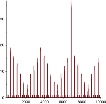
• 2. The result is true for other arbitrarily large gaps, for example, those where the second interval is far from any multiple of p ². Actually, the graph of the order of p in DT(I _g) as a function of g shows zones with higher and higher peaks that eventually reduce to 0 and rest there for an interval before growing again. We show here the graph for p = 23 and g up to 10,000.

  

• 3. Also we can consider three or more intervals of different lengths with different gaps between them. The condition on those gaps can be easily guessed looking at the graph of the sizes of the different classes mod p, as above, the simplest case being when the sum of the residues mod p of the lengths of the intervals and gaps is less that p.

• 4. There are several promising variations of the above. And it must be stressed that the condition p|DT(I) is necessary for I to be non-hyperbolic but is a long way from being sufficient, so many of the above examples can be hyperbolic even when the hypotheses fail. This gives many more examples of hyperbolic sets.

• 5. In [1] the authors study some cases where g = 1.

3.5 The Murty-Whang Criterion

In [19] the above DT(I) criterion is generalized to all n, using Representation Theory:

If I is non-hyperbolic then DT(I) is a linear combination of the prime factors of n with non-negative integer coefficients.

This allows a generalization of the examples in the previous section to situations where p odd is the smallest prime number dividing n (with restrictive extra hypotheses):

• (1’) Any subset of [1, …, p] is hyperbolic.

• (2’) Any subset of [1, …, 2p] consisting of indices of the same parity is hyperbolic, assuming that every other prime factor of n is greater that 2p − 1.

• (3’) For any two disjoint subsets of I ₁ and I ₂ of [1, …, p], the set I ₁ ∪ (I ₂ + kp) for $k\in \mathbb {N}$ is hyperbolic, provided every other prime factor of n is an upper bound for it.

• (4’) I _g in the theorem in the last section is hyperbolic with the same hypotheses if, further, every other prime factor of n is greater that p ² − 1.

4 Some Complex Varieties with Cyclic and Dihedral Symmetry

4.1 Some Complex Varieties with Cyclic Symmetry

Let ξ be an n-th root of unity, d > 1, an integer and consider the hypersurface in $\mathbb {C} P^{n-1}$ given by the equation:

$$\displaystyle \begin{aligned}\varSigma_{j=1}^{n} \xi^{j} z_j^d=0\end{aligned}$$

This variety is clearly smooth and invariant under a cyclic permutation of the coordinates z _j. Our varieties will be intersections of such hypersurfaces for different n-th roots of unity but same³ degree d > 1:

Let ρ be a primitive root of unity, K ⊂ [1, …, n] with m elements, d > 1 and $\mathcal {Z}(K)$ the projective variety with equations

$$\displaystyle \begin{aligned}\varSigma_{j=1}^{n} \rho^{ij} z_j^{d}=0,\,\, i\in K\end{aligned}$$

This is again invariant under the cyclic group and also invariant under the obvious action of $\mathbb {Z}_{d}^{n-1}$. Combining both actions we get a group of order nd ⁿ⁻¹. We will not consider this extended action for the moment, although it will be present in all the examples in this section.

For equations like these there is a simple criterion for smoothness:

Lemma 1

An intersection of hypersurfaces $V\subset \mathbb {C} P^{n-1}$ given by equations of the form

$$\displaystyle \begin{aligned}\varSigma_{j=1}^{n} A_j z_j^d=0\end{aligned}$$

with $A_j\in \mathbb {C}^m$ and d > 1 is smooth if, and only if, the m × n matrix A with columns A _j satisfies the property

(H) All ⁴ the m × m minors of A are different from zero.

Proof

Assume one m × m minor is zero with columns in J ⊂ [1, …, n]. This means that there are constants α _j for j ∈ J, not all zero, such that

$$\displaystyle \begin{aligned}\varSigma_{j\in J}\alpha_j A_j=0.\end{aligned}$$

A point $z\in \mathbb {C}^n$ such that z _j is a d-th root of α _j for j ∈ J and is 0 otherwise satisfies

$$\displaystyle \begin{aligned}\varSigma_{j=1}^{n} A_j z_j^d=\varSigma_{j\in J}\alpha_j A_j=0\end{aligned}$$

so it defines a point in $V\subset \mathbb {C} P^{n-1}$ where the jacobian matrix of the equations has columns $d z_j^{d-1} A_j$ which are zero for j∉J and a scalar multiple of A _j for j ∈ J. Since the latter are linearly dependent, the jacobian matrix at z has rank less than m and z is a singular point of V .

Reciprocally, if z is a singular point of V , let J be the set of indices such that z _j≠0.

If J has at least m elements, take any collection J′⊂ J of m of them. The columns $d z_j^{d-1} A_j$ for j ∈ J′ of the jacobian matrix of the equations are linearly dependent and so are the columns A _j of A for j ∈ J′ which are scalar multiples of them since all the corresponding factors $d z_j^{d-1}$ are non-zero and (H) fails.

If J has less than m elements then the equations themselves

$$\displaystyle \begin{aligned}\varSigma_{j\in J}z_j^d A_j=0\end{aligned}$$

show that the A _j with j ∈ J are linearly dependent and so is any collection of m columns of A that contain them. Again (H) fails.

Applying this to our symmetric variety $\mathcal {Z}(K)$ we see that it is smooth if, and only if, the minors V [K, J] of the matrix V _n are non-zero for all J ⊂ [1, …, n] with m elements. From the results of the last section we obtain:

Theorem 5

• (1) If n is prime, all the 2ⁿ intersections $\mathcal {Z}(K)$ are smooth.

• (2) For all n and m, all the intersections $\mathcal {Z}(K)$ , where K = [1, …, m] are smooth.

• (3) For all n, $\mathcal {Z}(K)$ is smooth if, and only if, the complementary $\mathcal {Z}(K^{c})$ is smooth.

• (4) If K is any of the hyperbolic examples described in the previous section, then $\mathcal {Z}(K)$ is smooth.

To these we should add all the K equivalent to the ones described in the theorem under the action of the affine Galois group, in particular any interval mod p. This gives many smooth examples as well as some non-smooth ones, but still does not give a simple criterion to decide if a given one is smooth or not.

We can get some general results if we change the question: given a smooth algebraic variety X, is it diffeomorphic to one that has cyclic symmetry?

If X is a smooth complete intersection of m hypersurfaces in $\mathbb {C} P^n$, all of degree d, we have a way to attack it: construct one of our examples with cyclic symmetry having the same degrees. If this one is also smooth, then it is diffeomorphic to X and we are finished! This is a consequence of

Thom’s principle

Any two smooth complete intersections of m hypersurfaces in $\mathbb {C} P^n$ with the same degrees are diffeomorphic.

This is because in the complex space of all collections of m hypersurfaces of a given degree, the set of those that are not transverse is given by algebraic equations and therefore has real codimension at least 2. Then any two smooth ones can be joined by a path consisting only of smooth ones and are therefore diffeomorphic.

So we are free to choose which equations to use and there is a good choice: take the first m rows of the Vandermonde matrix V _n:

Theorem 6

Any smooth complete intersection of hypersurfaces of degree d in $\mathbb {C} P^{n-1}$ is diffeomorphic to a smooth complete intersection of the same type that is invariant under the natural cyclic group of order n.

There are various results about the topology of smooth complete intersections from which one can determine in many cases the topology of these smooth varieties ([4, 14], among others.)

In the particular case m = n − 2 we can describe completely the topology of a complete intersection:

Theorem 7

For the surface S of Euler characteristic χ the following are equivalent (cf. [10] ):

• (i) χ is of the form:

  $$\displaystyle \begin{aligned} \chi=d^{n-2}(n-d(n-2))\end{aligned} $$

  for some positive integers n, d > 1.

• (ii) S is diffeomorphic to a smooth complete intersection of hypersurfaces of degree d in $\mathbb {C} P^{n-1}$.

• (iii) S is diffeomorphic to such a smooth complete intersection in $\mathbb {C} P^{n-1}$ invariant under the natural cyclic group of order n.

The equivalence of (i) and (ii) follows from the formula for the Euler characteristic of an algebraic curve which is a smooth complete intersection of hypersurfaces of degrees d ₁, d ₂, …, d _n−2 in $\mathbb {C} P^{n-1}$:

$$\displaystyle \begin{aligned} \chi=d_1 \dots d_{n-2}( n-(d_1 +\dots + d_{n-2}))\end{aligned} $$

This wonderful formula is not as well-known as it deserves. One of its consequences is that the Riemann surfaces of genus 2 and 7, for example, cannot be realized as smooth complete intersections. We learned it from a paper by Grujic [12], then found it again in one by Libgober and Wood [14]. See also [10]. A geometric proof was produced for us by Enrique Artal (private communication).

4.2 Some Complex Varieties with Dihedral Symmetry

The natural way to upgrade the above cyclic actions to a dihedral action is by asking that the variety is also invariant under conjugation.

To obtain that, we assume that for every equation we have also the one with conjugate coefficients. In other words: if i ∈ K then also n − i ∈ K. We will say in this case that K is balanced. So we have a much smaller set of examples of varieties with dihedral symmetry. Nevertheless, all the general smoothness results are valid for balanced varieties and we get many smooth types of intersections of hypersufaces with dihedral symmetry:

Theorem 8

• (1) If n is prime, all the 2^{⌊n∕2⌋+1} balanced intersections $\mathcal {Z}(K)$ are smooth.

• (2) For all n and m, all the intersections $\mathcal {Z}(K)$ , where K is a balanced interval, are smooth.

• (3) For all n, the complementary $\mathcal {Z}(K^c)$ of a balanced intersection $\mathcal {Z}(K)$ is also balanced, so one of them is smooth if, and only if, the other one is.

• (4) Many of the examples of Sect. 3.4 can be made to be balanced and give smooth examples. In particular, the examples I _g with two intervals of the same size, can be translated to be balanced for appropriate values of the gap g.

To apply this to the existence of smooth actions on smooth complete intersections of hypersurfaces of degree d, we need to see if there are enough balanced ones of a given degree and dimension. We obtain about three fourths of them:

Theorem 9

If n and m are not both even, then every smooth complete intersection of m hypersurfaces of degrees d in $\mathbb {C} P^{n-1}$ admits a smooth dihedral action.

This is because, if n = 2k + 1, there are balanced submatrices of any even number of rows around the center, with K an interval from [k, k + 1] up to [1, …, 2k]. The complementary intervals I ^c are also balanced so we get smooth varieties of all codimensions m.

When n = 2k we get again balanced submatrices of any odd number of rows around the center, with K an interval from [k] up to [1, …, 2k − 1]. But in this case the complementary K ^c is again odd unless K is empty.

For example, if n is even and m = 2, there are no balanced examples that are smooth, so the same goes for m = n − 2 and we get in this case no smooth algebraic curves with dihedral symmetry. For other even values of n and m we do not know any smooth balanced examples. Nevertheless, for n odd we can take K to be the complementary of the interval [(n − 1)∕2, (n + 1)∕2] to get a smooth balanced system. This gives about half of the surfaces with cyclic symmetry:

Theorem 10

The surface of Euler characteristic

$$\displaystyle \begin{aligned}\chi=d^{n-2}(n-d(n-2))\end{aligned}$$

for n > 1 odd is diffeomorphic to a smooth complete intersection of hypersurfaces of degree d in $\mathbb {C} P^{n-1}$ invariant under the natural dihedral group.

There are many known examples of Riemann surfaces with cyclic or dihedral symmetry (see [5]), so our examples could be just new constructions of known cases. Maybe the interest of our examples lies in the fact that we realize them embedded in standard linear actions of specific dimensions and forming part of towers of varieties with the same groups acting.

5 Intersections of Real Affine Ellipsoids with Dihedral Symmetry

For the real analogs of the previous complex varieties

$$\displaystyle \begin{aligned}\varSigma_{j=1}^{n}A_j x_j^d=0\end{aligned}$$

where now $A_j\in \mathbb {R}^m$, to describe their topology we can restrict to the case d = 2, even in the non-smooth case:

For d odd, the homeomorphism of $\mathbb {R}^n$ to itself sending x _i to $x_i^d$ restricts to a homeomorphism between the variety and the linear variety corresponding to d = 1, whose topology is evident.

For d = 2k, it is the homeomorphism of $\mathbb {R}^n$ to itself sending x _i to $sign(x_i) x_i^k$ that establishes a homeomorphism between the variety and the variety corresponding to d = 2. So for the topological description it is enough to consider this case.

The smoothness condition for a system with d even is now weaker than hyperbolicity: if we have a real linear dependence between m or less columns of the matrix of coefficients of a system

$$\displaystyle \begin{aligned}\varSigma_{j\in J}\alpha_j A_j=0,\end{aligned}$$

we can not obtain a critical point of the variety as in Sect. 4 by taking the d-th roots of the α _j, unless they are all non-negative. So now what we have to avoid is that there are m or less columns in the matrix such that a positive linear combination of them is zero. Or, equivalently, to ask that no convex combination of them is zero. This condition is called Weak Hyperbolicity:

(WH) An m × n real matrix is called weakly hyperbolic if the origin in $\mathbb {R}^m$ is not a convex combination of m of its columns.

A detailed proof of the equivalence between (WH) and smoothness for d = 2 can be found in [17]. It works for any even d, and equally well for the projective version and for the affine one outside the origin or intersected with the unit sphere. It is in the last case that progress on the topological description has been obtained in large families of them (described in the introduction), so it is there that we can hope to apply the results of Sect. 3.

Now we can look at the examples with dihedral symmetry mentioned in the introduction:

Take K ⊂ [1, …, [n∕2]] of cardinality m and Z(K) be the variety

$$\displaystyle \begin{aligned}\varSigma_{i=1}^n \rho^{ki} x_i^2=0,\,\,\,k\in K\end{aligned}$$

$$\displaystyle \begin{aligned}\varSigma_{i=1}^n x_i^2=1\end{aligned}$$

Each of the homogeneous equations is actually a pair of real equations (taking real and imaginary parts of the coefficients), with the exception, when n is even and n∕2 ∈ K, of the last one which has real coefficients 1 and − 1. So, if we denote by $\hat {m}$ the number of real homogeneous equations, $\hat {m}=2m$ in general case and $\hat {m}=2m-1$ in the exceptional case.

The $\hat {m}\times n$ matrix of coefficients of this system is equivalent by real row operations to the balanced submatrix of V _n formed by adding to the rows their complex conjugate rows. So the question of the weak hyperbolicity of these two matrices are equivalent.

The theory of weak hyperbolicity of submatrices of V is still to be developed. But we can use the fact that this property is implied by hyperbolicity and use all the positive results of Sect. 3 to obtain results about the smoothness of Z(K). It must be remembered that for a smooth Z(K) its matrix may not be hyperbolic. This would mean that its complex version would have only imaginary singularities.

The complementary matrix should be taken inside the range [1, …, [n∕2]] of rows so even after taking the balanced equations it corresponds to complementarity in the range [1…, n − 1]. So it does not correspond to complementarity inside the range [1…, n] for which we understand the duality of smoothness. The complementary of hyperbolicity in this case is a property that can be called affine hyperbolicity, meaning that no collection of $\hat {m}+1$ columns lie in an affine subspace. The property that is complementary (in this new sense) to weak hyperbolicity has not been characterized so far. Still, the duality between the combinatorial objects associated to Z(K) and Z(K ^c) describe in the introduction is a solid fact that needs to be understood.

We summarize the main positive results about the smoothness of Z(K):

Theorem 11

• (1) For all n, if I is an interval containing [n∕2], then Z(K) is smooth.

• (2) If n is prime, all the 2^[n∕2] intersections Z(K) are smooth.

• (3) If n = p ^k and K is an interval, then Z(K) is smooth, provided K and its conjugate interval satisfy the conditions of Theorem 4 with ℓ ₁ = ℓ ₂ and g the gap between them.

Case 1 looks interesting because for each n we have actually a tower of varieties with dihedral symmetry, namely, all those corresponding to the intervals [k, …, [n∕2]] for k from 1 to [n∕2]. The varieties in this tower have even dimensions going from 0 to n − 2. They give also towers of polytopes with the same symmetry and dimensions. These are for the moment the only examples for which we have explored their topology:

For the cases k = 1, k = 2 and k = [n∕2] their topology is known from the results (A) and (B) mentioned in the introduction: they are all connected sums of sphere products, connected up to the middle dimension.

Long computations of faces of the corresponding polytopes give always that their duals are neighbourly, which means that the varieties are again connected sums of sphere products, connected up to the middle dimension. The number of summands for small k grows very fast with n (recall the genus of the surfaces in part B) of the introduction.

One can conjecture that this is true for all n. If this is so, we would have interesting towers of highly connected varieties and of neighborly polytopes with dihedral symmetry. The proof of this conjecture seems to imply an even deeper understanding of the properties of the minors of the DFT matrix.

References

Achanta, H.K., Biswas, S., Dasgupta, B.N., Dasgupta, S., Jacob, M., Mudumbai, R.: The spark of Fourier matrices: Connections to vanishing sums and coprimeness. Digital Signal Process. 61, 76–85 (2017)
Alexeev, B., Cahill, J., Mixon, D.G.: Full spark frames. J. Fourier Anal. Appl. 18(6), 1167–1194 (2012)
Al-Raisi, A.: Equivariance, Module Structure, Branched Covers, Strickland Maps and Cohomology Related to the Polyhedral Product Functor. Ph.D. Thesis, University of Rochester (2014)
Browder, W.: Complete intersections and the Kervaire invariant. Lect. Notes Math. 763, 88–108 (1979)
Bujalance, E., Cirre, F.J., Gamboa, J.M., Gromadzki, G.: Symmetries of Compact Riemann Surfaces. Lecture Notes in Mathematics, vol. 2007, pp. xx+158. Springer, Berlin/Heidelberg (2010)
de la Vega, G., López de Medrano, S.: Generalizing the May-Leonard system to any number of species. In: Proceedings of the International Conference Dynamical Systems: 100 Years After Poincaré, Gijón, Spain, Springer Proceedings in Mathematics and Statistics, vol. 54, pp. 395–407 (2013)
Dieudonné, J.: Une propriété des racines de l’unité, Collection of articles dedicated to Alberto González Domínguez on his sixty-fifth birthday. Rev. Un. Mat. Argentina 25, 1–3 (1970/1971)
Gitler, S., López de Medrano, S.: Intersections of quadrics, moment-angle manifolds and connected sums. Geom. Topol. 17(3), 1497–1534 (2013)
Gómez Gutiérrez, V., López de Medrano, S.: Stably parallelizable compact manifolds are complete intersections of quadrics. Publicaciones Preliminares del Instituto de Matemáticas, UNAM (2004)
Gómez Gutiérrez, V., López de Medrano, S.: Surfaces as complete intersections. In: Riemann and Klein Surfaces, Automorphisms, Symmetries and Moduli Spaces. Contemporary Mathematics, vol. 629, pp. 171–180. AMS, Providence (2014)
Gómez Gutiérrez, V., López de Medrano, S.: Topology of the intersections of quadrics II. Bol. Soc. Mat. Mex. 20(2), 237–255 (2014)
Grujić, V.N.: ξ y-characteristics of projective complete intersections. Publicatons de l’Institut Mathématique, nouvelle série 74(88), 19–23 (2003)
Hirzebruch, F.: Arrangements of lines and algebraic surfaces. In: Arithmetic and Geometry. Progress in Mathematics 36, vol. II, pp. 113–140. Boston: Birkhauser (1983)
Libgober, S., Wood, J.W.: Differentiable structures I. Topology 21(4), 469–482 (1982)
López de Medrano, S.: The space of Siegel leaves of a holomorphic vector field. In: Holomorphic Dynamics (Mexico, 1986). Lecture Notes in Mathematics, vol. 1345, pp. 233–245 Springer, Berlin (1988)
López de Medrano, S.: The topology of the intersection of quadrics in \(\mathbb {R}^{n}\). In: Algebraic Topology (Arcata, 1986). Lecture Notes in Mathematics, vol. 1370, pp. 280–292. Springer, Berlin (1989)
López de Medrano, S.: Singular intersections of quadrics I. In: Singularities in Geometry, Topology, Foliations and Dynamics- A Celebration of the 60th Birthday of José Seade. Trends in Mathematics, pp. 155–170. Birhäuser, Basel (2016)
Murty, M.R., Whang, J.P.: The uncertainty principle and a generalization of a theorem of Tao. Linear Algebra Appl. (2012). https://doi.org/doi:10.1016/j.laa.2012.02.009
Stevenhagen, P., Lenstra, H.W.: Chebotarëv and his density theorem. Math. Intelligencer 18(2), 26–36 (1996). Springer
Tao, T.: An uncertainty principle for cyclic groups of prime order. Math. Res. Lett. 12(1), 121–127 (2005)
Acknowledgements
Conversations with Enrique Artal, Pablo Barrera, Shirley Bromberg, Peter Bürgisser, Sylvain Cappell, Marc Chaperon, Antonio Costa, Genaro de la Vega, Javier Elizondo, Matthias Franz, Ignacio Luengo, Mike Shub, Denis Sullivan, Yuri Tschinkel, Luis Verde, Alberto Verjovsky, Felipe Zaldívar and Adrián Zepeda have been very helpful.
Special mention is deserved by Matthias Franz who has dedicated a great effort to the Vandermonde minors question. Long discussions with him have clarified many aspects of the theory (and of the present paper) and the proof of Theorem 2 is due to him. Much joint work is still in progress and will certainly be the object of a joint future paper more closely related to his interests and point of view.
This work was partially supported by a Papiit-UNAM grant IN111415.
Author information
Authors and Affiliations
Corresponding author
Editor information
Editors and Affiliations
Rights and permissions
Copyright information
© 2018 Springer Nature Switzerland AG
About this chapter
Cite this chapter
López de Medrano, S. (2018). Smoothness in Some Varieties with Dihedral Symmetry and the DFT Matrix. In: Greuel, GM., Narváez Macarro, L., Xambó-Descamps, S. (eds) Singularities, Algebraic Geometry, Commutative Algebra, and Related Topics. Springer, Cham. https://doi.org/10.1007/978-3-319-96827-8_16
Download citation
DOI: https://doi.org/10.1007/978-3-319-96827-8_16
Published:
Publisher Name: Springer, Cham
Print ISBN: 978-3-319-96826-1
Online ISBN: 978-3-319-96827-8
eBook Packages: Mathematics and StatisticsMathematics and Statistics (R0)