Dataflow Modeling for Reconfigurable Signal Processing Systems

Abstract

Nowadays, adaptive signal processing systems have become a reality. Their development has been mainly driven by the need of satisfying diverging constraints and changeable user needs, like resolution and throughput versus energy consumption. System runtime tuning, based on constraints/conditions variations, can be effectively achieved by adopting reconfigurable computing infrastructures. These latter could be implemented either at the hardware or at the software level, but in any case their management and subsequent implementation is not trivial. In this chapter we present how dataflow models properties, as predictability and analyzability, can ease the development of reconfigurable signal processing systems, leading designers from modelling to physical system deployment.

These keywords were added by machine and not by the authors. This process is experimental and the keywords may be updated as the learning algorithm improves.

1 Reconfigurable Signal Processing Systems

For many years, the design of a signal processing system was mostly driven by performance requirements. Hence, design effort was mainly focused on optimizing the throughput and latency of the designed system, while satisfying constraints of reliability and quality of service, and minimizing the system production cost. In this context, a strong predictability of system behavior is essential, especially when designing safety-critical real-time systems. Many compile-time methodologies, computer-aided design tools, and static Models of Computation (MoCs), such as the decidable dataflow MoCs [26], have been created to assist system designers in reaching these goals.

In recent years, the ever increasing complexity of signal processing systems has lead to the emergence of new design challenges. In particular, modern signal processing systems no longer offer a fixed throughput and latency, specifically tuned to satisfy all timing constraints in the most demanding scenarios from the system specification. Instead, modern systems must now dynamically adapt their behavior on-the-fly to satisfy strongly varying workloads and performance objectives, while optimizing new design goals such as minimizing use of shared computational resources, or minimizing power consumption. These variations of the workload and performance objectives may be induced by functional and non-functional requirements of the system. An example of system with strongly varying functional requirements is the computing system managing a base station of the Long-Term Evolution (LTE) telecommunication network. Every millisecond, the bandwidth allocated for up to 100 active users connected to the managed antenna may change [50], with a strong impact on the amount and nature of computations performed by the system. An embedded video decoding system that lowers the quality of its output in order to augment battery life is an example of varying non-functional requirement [48, 55]. As presented in [64], increasing the dynamism of a signal processing often results in a partial loss of predictability, making it difficult, and sometimes impossible, to guarantee the real-time performance or the reliability (e.g. deadlock freedom) of a system.

The purpose of reconfigurable signal processing systems is to offer a carefully balanced trade-off between system predictability and adaptivity. This trade-off between diverging properties is essential to meet classical constraints of system performance and reliability while satisfying varying requirements of modern system. To offer a trade-off between predictability and adaptivity, reconfigurable systems rely both on design-time analysis and optimization of system behavior, that make it possible to predict the system behavior, and on runtime management technique that enable system adaptation.

The objective of this chapter is to present how the analyzability of dataflow MoCs can be exploited to ease the development of reconfigurable signal processing systems. The chapter structure is briefly summarized as follows: Sect. 2 presents how reconfigurable systems can be efficiently modeled with dedicated dataflow MoCs, and Sects. 3 and 4 presents how software and hardware techniques, respectively, can be used to implement reconfigurable applications efficiently. In more details, Sect. 2 formally introduces the concept of reconfigurable dataflow MoCs and discusses its key differences with decidable and dynamic classes of dataflow MoCs. This concept is illustrated through the semantics of several reconfigurable dataflow MoCs. In Sect. 3, software implementation techniques supporting the execution of reconfigurable dataflow application are presented. This section covers a wide range of software implementation techniques, spanning from compile-time optimizations to runtime management system for reconfigurable applications. Then, Sect. 4 presents a summary on reconfigurable computing systems, where both coarse grained and fine grained reconfiguration paradigm are addressed describing how dataflow MoCs may help in mapping and managing this kind of highly flexible computing systems.

2 Reconfigurable Dataflow Models

The high abstraction level of dataflow MoCs makes them popular models for specifying complex signal processing applications [26]. By exposing coarse-grain computational kernels,¹ the actors, and data dependencies between them, the First-In First-Out queues (Fifos), the dataflow semantics eases the specification of parallel applications, and provides necessary formalism for many verification and optimization techniques for the design of signal processing systems.

The expressiveness of a MoC defines the range of applications behavior this MoC can describe. The expressiveness of a dataflow MoC is directly related to its firing rules, which are used to specify how and when actors produce and consume data tokens on connected Fifos. Dataflow MoCs can be sorted into three classes depending on their expressiveness:

• Decidable dataflow MoCs [26]: all production and consumption rates are fixed at compile-time, either as fixed scalar, or with periodic variations. The key characteristics of decidable dataflow graphs is that, through an analysis of data rates, it is possible to derive a schedule of finite length at compile-time.

• Dynamic dataflow MoCs [64]: production and consumption rates can change non-deterministically at each actor firing, making these models Turing-complete ones. Hence, for most dynamic dataflow MoCs, schedulability, deadlock-freedom, real-time properties, and memory boundedness of application graphs can be verified neither at compile-time, nor at runtime. In some dynamic dataflow MoCs, this lack of analyzability is partially alleviated through specialization of the model semantics.

• Reconfigurable dataflow MoCs: production and consumption rates can be reconfigured (i.e. changed) non-deterministically at restricted points in application execution. These MoCs are sometimes also called parametric dataflow MoCs [11]. This restriction limits the expressiveness of reconfigurable dataflow models, but makes it possible to verify application properties, like schedulability, either at compile-time or at runtime, after a reconfiguration occurred.

The following subsections formally introduce the reconfiguration semantics behind reconfigurable dataflow MoCs, and shows how it benefits model analyzability through the presentation of several reconfigurable dataflow MoCs. Implementation optimization techniques taking advantage of the reconfiguration semantics are presented in Sects. 3 and 4.

2.1 Reconfiguration Semantics

The reconfiguration semantics behind reconfigurable dataflow MoCs is a mathematical model that makes it possible to detect potentially unsafe reconfigurations of an application graph [44]. A reconfiguration is said to be unsafe if it may result in an unwanted and undetected state of the application, such as a deadlock or an inconsistence in production and consumption rates.

The reconfiguration semantics for dataflow MoCs is based on the definition of hierarchical actors, parameters, and quiescent points. The reconfiguration semantics can be implemented by any dataflow MoC with atomic actor firings. This assumption guarantees the applicability of the reconfiguration semantics to a broad range of dataflow MoCs, including decidable [26], multi-dimensional [33], and some dynamic dataflow MoCs [64].

Formally, a hierarchical graph is defined as a set of actors A. An actor a ∈ A can either be an atomic actor, an actor whose internal behavior is specified with host code, or a hierarchical actor, an actor whose internal behavior is specified with a subset of actors A _a ⊂ A. The top-level graph itself is considered as a hierarchical actor with no parent, and that contains all other actors in A. Each actor a is associated to a dedicated set of parameters P _a, that can influence both its production and consumption rates, and the computations it performs. At any point in execution time, each parameter p ∈ P (=⋃_{a ∈ A} P _a) is associated to a value given by a valuation function: val(p) whose type (e.g. integer, real, boolean, ...) depends on the underlying model semantics. The value val(p) of a parameter may be independent, or may depend on the value of one or several other parameters in P. The transitive relation q depends on p, between two parameters p ≠ q, is noted $p \rightsquigarrow q$. Reconfiguration occurs when the value of an independent parameter is modified during the execution of the application.

Figure 1 shows an example of graph specified with a synthetic dataflow MoC implementing the reconfiguration semantics. Figure 1a illustrates the semantics, which is then used to build up the example in Fig. 1b. The graph of Fig. 1b consists of five actors, including one hierarchical actor h that contains two atomic actors C and D. Each consumption and production rate is defined by a dedicated parameter whose valuation function is specified as an expression written next to the graph. In this graph, p, s, and t are independent parameters and all other parameters have dependencies; as for example $p \rightsquigarrow r$.

Fig. 1

Synthetic dataflow MoC implementing the reconfiguration semantics. (a) Semantics. (b) Graph and current valuation of parameters

Reconfiguration semantics models as a quiescent point the state of an actor between two firings. Like actor firings, the set of quiescent points Q _a of an actor a is ordered in time according to a transitive precedence relation. Since firings of actors contained in a hierarchical subgraph cannot span over multiple firings of their enclosing actor, when a hierarchical actor is quiescent, all actors contained in its hierarchy must also be. A graphical representation of quiescent points for the graph of Fig. 1 is presented in Fig. 2.

Fig. 2

Abstract representation of the quiescent points for the graph of Fig. 1. Vertical lines represent quiescent points of actors. Dotpoint arrows represent actor firings and define a partial ordering of quiescent points

The reconfiguration semantics requires reconfigurations of any independent parameter p ∈ P to happen only during a quiescent points q ∈ Q(=⋃_{a ∈ A} Q _a) at execution time. The set of parameters reconfigured during a quiescent point q is noted: R(q) ⊆ P.

When using a dataflow MoC implementing the reconfiguration semantics, a compile-time analysis of parameters and quiescent points of an application graph can be used to verify model-specific reconfiguration safety requirements [44]. Safety requirements of a dataflow MoC are expressed as statements in the form “Parameter p is constant over firings of actor a”. Formally:

Definition 1

Parameter p is constant over firings of actor c if and only if $\forall a \in A, \forall q\in Q_a, \forall r\in R(q), r \rightsquigarrow p \Rightarrow q \in Q_c$.

For example, in the Synchronous Dataflow (SDF) MoC, decidability can be expressed as the following safety requirement: all parameters are required to be constant over firings of the top-level actor.

In [11], Bouakaz et al. present a Survey of dataflow MoCs adopting the reconfiguration semantics. Next sections present examples of MoCs implementing the reconfiguration semantics.

2.2 Reconfigurable Dataflow Models

2.2.1 Hierarchy-Based Reconfigurable Dataflow Meta-Models

The purpose of a dataflow meta-model is to bring new elements to the semantics of a base dataflow MoC in order to increase its modeling capabilities. The Parameterized and Interfaced Dataflow Meta-Model (PiMM) [17] and Parameterized Dataflow [8] are two dataflow meta-models with similar purpose: bring hierarchical graph composition and safe reconfiguration features to any decidable dataflow MoC that has a well-defined notion of graph iteration and repetition vector, such as SDF and Cyclo-Static Dataflow (CSDF) [26], or Multi-Dimensional SDF (MDSDF) [33]. A base dataflow MoC whose semantics is enriched with PiMM or with the parameterized dataflow meta-model is renamed with prefixes π- and P-, respectively. For example, Parameterized and Interfaced SDF (πSDF) and Parameterized SDF (PSDF) are the reconfigurable generalizations of the decidable SDF MoC.

In PiMM and parameterized dataflow meta-models, safe reconfiguration is expressed as a local synchrony requirement [8]. Intuitively, local synchrony requires the repetition vector of the subgraph of a hierarchical actor to be configured at the beginning of the execution of this subgraph, and to remain constant throughout a complete graph iteration, corresponding to a firing of the parent actor. Hence, in locally synchronous hierarchical subgraph, all parameters influencing production and consumption rates of actors must remain constant over the firing of their parent actor. Formally, with S _c, the set of direct child actors of a hierarchical actor c ∈ A, where direct child means that ∀h ∈ S _c, d ∈ S _h ⇒ d∉S _c.

Definition 2

Subgraph S _c of actor c ∈ A, is locally synchronous if and only if: ∀a ∈ S _c, ∀p ∈ P _a, the requirement “p is constant over firings of c” is verified.

The semantics of PiMM, which is an evolution of the parameterized dataflow semantics, is illustrated in Fig. 3. An example of πSDF graph is given in Fig. 4.

Fig. 3

Semantics of the Parameterized and Interfaced Dataflow Meta-ModelPiMM

Fig. 4

Example of πSDF graph. Bit processing algorithm of the Physical Uplink Shared Channel (PUSCH) decoding of the LTE telecommunication standard [17]

In PiMM, graph compositionality is supported by hierarchical actors, as defined in the reconfiguration semantics, and by data interfaces. The purpose of interface-based hierarchy [52] is to insulate the nested levels of hierarchy in terms of graph consistence analysis. To do so, data interfaces automatically duplicate and discard data tokens if, during a subgraph iteration, the number of tokens exchanged on Fifos connected to interfaces is greater than the number of token produced on the corresponding data ports of the parent actor.

The parameterization semantics of PiMM consists of parameters and parameter dependencies as new graph elements, and configuration input ports and interfaces as new actor attributes. The value associated to a parameter of a graph is propagated through explicit parameter dependencies to other parameters and to actors. In the πSDF MoC, it is possible to disable all firings of an actor by setting all its production and consumption rates to zero. As illustrated in Fig. 4, parameter values can be propagated through multiple levels of hierarchy using a configuration input port on a hierarchical actor and a corresponding configuration input interface in the associated subgraph.

The reconfiguration semantics of PiMM is based on actors with special firing rules, called configuration actors. When fired, reconfiguration actors are the only actors allowed to dynamically change the value of a parameter in their graph. As a counterpart for this special ability, reconfiguration actors must be fired exactly once per firing of their parent actor, before any non-configuration actor of their subgraph. This restriction is essential to ensure the safe reconfiguration of the subgraph to which configuration actors belong. To be strictly compliant with Definition 2, configuration actors and other actors of a subgraph can be considered as two separate subgraphs, executed one after the other.

The local synchrony requirement of the πSDF MoC naturally enforces the predictability of the model. After firing all configuration actors of a subgraph, all parameters values, and hence all actor production and consumption rates of this subgraph, are known and will remain fixed for a complete subgraph iteration. Runtime analyses and optimization techniques can be used to compute the repetition vector of the subgraph, to optimize the mapping and scheduling of actors, to allocate the memory, or to verify that future real-time deadlines will be met. An important benefit of this predictability is the support for data-parallelism which is often lost in dynamic dataflow MoCs. Data parallelism consists in starting several firings of the same actor in parallel if enough data tokens are available. Data-parallelism is supported only if the next sequence of firing rates is know a priori, as is the case in πSDF graphs. In dynamic dataflow MoCs [64], the firing rules of an actor generally depend on its internal state after completion of its previous firing. This internal dependency between actor firings forces their sequential execution, thus preventing data parallelism.

Figure 4 presents a πSDF specification of the bit processing algorithm of the Physical Uplink Shared Channel (PUSCH) decoding which is part of the LTE telecommunication standard. The LTE PUSCH decoding is executed in the physical layer of an LTE base station (eNodeB). It consists of receiving multiplexed data from several User Equipments (UEs), decoding it and transmitting it to upper layers of the LTE standard. Because the number of UEs connected to an eNodeB and the rate for each UE can change every millisecond, the bit processing of PUSCH decoding is inherently dynamic and cannot be modeled with static MoCs such as SDF. Further details on this application, and specification using the parameterized dataflow meta-model, can be found in [50].

Compile-time and light-weight runtime scheduling technique for executing πSDF and PSDF graphs, are presented in Sect. 3. Combination of the parameterized dataflow semantics and the CSDF MoC is studied in [32] for the design of software-defined radio applications.

2.2.2 Statically Analyzable Reconfigurable Dataflow Models

Schedulable Parametric Dataflow (SPDF) and Boolean Parametric Dataflow (BPDF) are non-hierarchical reconfigurable generalizations of the SDF MoC that emphasize static model analyzability. In particular, the semantics of the SPDF and BPDF MoCs make it possible to verify safe reconfiguration requirements and to guarantee graph consistency and liveness at compile time. In πSDF and PSDF, although local synchrony can be checked at compile time, consistency and liveness of a subgraph can only be verified at runtime, after configuration of all the parameters contained in this subgraph.

In the SPDF MoC semantics, symbolic parameters P with integer values in $\mathbb {N}^*$ are used for parameterization. Special actors, called modifiers, have the ability to dynamically change the value of a symbolic parameter. To ensure safe reconfiguration, a modifier m ∈ A will set a new value for a parameter p ∈ P with a pre-defined change period $\alpha \in \mathbb {N}^*$. In practice, this means that the value of p will be changed every α firings of m. In an SPDF graph, as shown in Fig. 5, the annotation “set p[α]” is used to denote that an actor is a modifier of parameter p, with change period α. Change periods, and production and consumption rates of actors are specified with products $\prod _{i = 0}^{n} e_i$, where e _i is either an integer in $\mathbb {N}^*$, or a symbolic parameter p ∈ P.

Fig. 5

Example of Schedulable Parametric DataflowSPDF graph

Using balance equations of actor production and consumption rates, similar to those used for SDF graphs [26], graph consistency can be verified, and a symbolic repetition vector can be computed. The basic operation used to find the symbolic repetition vector of an SPDF graph is the computation of the Greatest Common Divisor (GCD) of the numbers of data tokens produced and consumed on each Fifo of the graph. Using this GCD, the numbers of repetition of the producer and consumer actors, relatively to each other, can be deducted by dividing the rates of the actors by this GCD. For example, in the graph of Fig. 5, the GCD of the Fifo between actor D and E is gcd _DE = gcd(q, 2pq) = q, which means that actor E will be executed rate _D∕gcd _DE = 2pq∕q = 2p times for each rate _E∕gcd _DE = q∕q = 1 execution of actor D. Using this principle, an algorithm detailed in [22] can be used to compute the parametric number of repetition of all actors in an SPDF graph. Using this algorithm on the SPDF graph of Fig. 5, the following symbolic repetition vector is obtained: A ³ B ^6p C ⁹ D ^12p E ⁶ F, where X ^a means that actor X is fired a times per iteration of the graph. Notation #X is used to denote the repetition count of an actor X ∈ A. Similarly, liveness (i.e. deadlock-freedom) of graphs can be verified statically with an analysis of cyclic data-paths inspired from SDF graph techniques.

Reconfiguration safety in SPDF graphs is based on the notion of parameter influence region. The influence region R(x) of a parameter x is the set of: a) Fifos whose rates depend on x, b) actors connected to these Fifos, and c) actors whose numbers of repetitions depend on x. For example in Fig. 5, R(q) comprises Fifo DE and actors D and E; and R(p) comprises the whole graph except actor F and Fifos connected to it.

Two safe reconfiguration requirements are used in SPDF: data and period safety. Intuitively, data safety requires that the region R(p) influenced by a parameter p ∈ P comes back to an initial state, in terms of the number of data-tokens on Fifos, between each reconfiguration of p. In other words, data safety requires the (virtual) subgraph composed by R(p) to complete a kind of local iteration and be quiescent when a reconfiguration of a parameters influencing it occurs. Formally, data safety requires that ∀p ∈ P, with modifier m ∈ A and change period α, all actors a ∈ R(p) have a repetition count #a such that gcd(#a, #m∕α) = #m∕α (i.e. #a is a multiple of #m∕α). For example in Fig. 5, with actor E ∈ R(q) and modifier B annotated “set q[2p]”, actor E is data safe since #E = 6 is a multiple of #B∕2p = 6p∕2p = 3.

Period safety restricts how often a parameter q can be reconfigured by its modifier m if #m itself depends on a parameter p. In this case, period safety ensures that q is reconfigured at least as often as the start of a new iteration of the subgraph formed by R(p). Formally, ∀p, q ∈ P with modifiers m _p and m _q, change period α _p and α _q, and #m _q depending on p, period safety requires #m _q∕α _q to be a multiple of #m _p∕α _p. If this condition is not met, reconfiguration of q may happen in the middle of an iteration of the subgraph formed by R(p), when it is not quiescent. For example, in Fig. 5, repetition count #B = 6p of the emitter of q depends on p, but its change period is safe since #B∕2p = 3 is a multiple of #A∕1 = 3. With the period of q set to 3p instead, the graph would remain data safe but would no longer be period safe, as #B∕3p = 2 is not a multiple of #A∕1 = 3. A consistent, data and period safe SPDF graph will always be schedulable in bounded memory [22].

The semantics of the BPDF MoC is closely related to the one of the SPDF MoC, and provides the same advantages in terms of static graph analyzability [6]. The main difference between the two MoCs is that reconfigurable integer parameters of SPDF are replaced with reconfigurable boolean parameters in BPDF. Through combinational logic expressions, these boolean parameters are used to change the BPDF graph topology, by enabling and disabling Fifos. This feature is equivalent to setting data rates to 0 in the SPDF and πSDF MoCs.

Examples of SPDF and BPDF graphs of multimedia, signal processing, and software defined radio applications can be found in [6, 16, 22]. Compilation techniques for deploying SPDF graphs onto multi and many-core architecture will be presented in Sect. 3.

2.3 Dynamic Dataflow MoCs and Reconfigurability

In dynamic dataflow MoCs, as presented in [64], production and consumption rates of actors may change dynamically at each firing, depending on the firing rules specified for each actor. In most dynamic dataflow MoCs, the semantics include elements to specify explicitly the internal firing rules of each actor. A common way to characterize firing rules of a dynamic actor is to model its internal state with a Finite State Machine (FSM), or a similar model like a Markov chain, and to associate each FSM state with pre-defined production and consumption rates for each data port. These FSMs can be specified either explicitly by the application designer, using a dedicated language, as in the Scenario-Aware Dataflow (SADF) and Core-Functional Dataflow (CFDF) MoCs [40, 64], or implicitly in the language describing the internal behavior of actors, as in frameworks based on the CAL Actor Language (CAL) [13, 21, 67].

An example of dynamic dataflow graph with associated FSMs is presented in Fig. 6. This graph represents the residual decoding of macro-blocs of pixels in a video decoding application. The semantics used for the FSMs presented in Fig. 6b, c is similar to the one of the CFDF MoC. Each state of the FSMs is associated with an integer production and consumption rate for each port of the corresponding actor. When enough data tokens are available on the input Fifos according to the current actor state, the actor is fired and one state transition is traversed, thus deciding the next firing rule.

Fig. 6

Dynamic dataflow graph inspired by the residual decoding of a video decoder. (a) Dynamic dataflow graph. (b) FSM of the VLC actor. Prod./Cons. rates for each state are expressed in the following order bits;cfg;mbo. (c) FSM of the Q ⁻¹ and DCT ⁻¹ actors. Prod./Cons. rates for each state are expressed in the following order cfg;mbi;mbo

In the graph of Fig. 6, the Variable Length Code (VLC) actor is responsible for decoding the information corresponding to each macroblock (i.e. square of pixel) from the input bitstream. To do so, the VLC actor reads the input bitstream bit-by-bit in the Recv state, and fills an internal buffer. When enough bits have been received, the VLC actor detects it, and goes to the 16×16 or 32×32 state, depending on the dynamically detected macroblock size. In the 16×16 or 32×32 states, the VLC actor produces a configuration data-tokens on its cfg port, and quantized macroblock coefficients on its mb port. The configuration data-token is received by the dequantizer actor Q ⁻¹ and the inverse discrete cosine transform actor DCT ⁻¹, which successively process the quantized macroblock coefficients in the state corresponding to the dynamically detected macroblock size: 16×16 or 32×32.

Although dynamic dataflow MoCs inherently lack the predictability that characterize reconfigurable dataflow MoCs, several techniques make it possible to increase the predictability of a dynamic dataflow graph in order to enable a reconfigurable behavior. The common point between these techniques, is that they exploit the actor behavioral information specified with FSMs in order to make parts of the application reconfigurable. Two different approaches are presented hereafter: in Sect. 2.3.1 classification techniques are used to identify reconfigurable behavior in application graphs specified with existing dynamic MoCs, and in Sect. 2.3.2, semantics of dynamic dataflow MoCs is extended to ease specification of reconfigurable behavior within dynamic applications. Further hardware reconfigurable implementation techniques based on dynamic dataflow MoCs are introduced in Sect. 4.

2.3.1 Classification of Dynamic Dataflow Graphs

The basic principle of classification techniques for dynamic dataflow graphs is to analyze the internal FSM of one or more actors in order to identify patterns that correspond to statically decidable behaviors. Here, a pattern designates a sequence of firings of one or more actors that, when started, will always be executed deterministically when running the application, despite the theoretical non-deterministic dynamism of the dataflow MoC.

In the example of Fig. 6, an analysis technique can detect two sequences of actor firings, corresponding to the processing of a macroblock of size 16×16 and 32×32, respectively. The first sequence is triggered when the VLC actor fires in the 16×16 state, which will always be followed by two firings of each of the Q ⁻¹ and DCT ⁻¹ actors, in the Cnfg and MB16 states. The second sequence is similar for the 32×32 configuration.

In [13], Boutellier et al. propose a technique to analyze a network of actors specified with CAL, and detect static sequences of actor firings in their FSMs. Once detected, each alternative sequence of actor firings is transformed into an equivalent SDF subgraph. Similarly to what is done in reconfigurable dataflow MoCs, SDF subgraphs are connected using switch/select actors capable of triggering dynamically an iteration of a selected SDF subgraph. As shown in [13], application performance can be substantially improved by exploiting the predictability of SDF subgraphs to decrease the overhead of dynamic scheduling of actor firings.

In [21], Ersfolk et al. introduce a technique to characterize dynamic actor by identifying the control tokens of the application. A control token is defined as a data token whose value is used in actor code to dynamically decide which firing rule will be validated for the next actor firing. For example, in Fig. 6, the data tokens exchanged on the cfg ports are control tokens, as they decide the next firing rules for the Q ⁻¹ and DCT ⁻¹ actors. Once a control token is identified, the data and control path influencing its value is backtracked both through graph Fifos and by applying an instruction-level dependency analysis to actor CAL code. By analyzing the datapath of control tokens, complex relations between firing rules of different actors can be revealed. As in the previous technique, these relations between firing rules of dynamic actors can be exploited to transform some part of a dynamic dataflow graph into an equivalent reconfigurable graph.

There exist several other techniques whose purpose is to detect reconfigurable or static behavior from a dynamic dataflow description. In [67], a set of rules are specified to classify the behavior of individual actors as static, cyclo-static, quasi-static, time-dependent (i.e. non-deterministic), and dynamic. These rules can be verified either by analyzing the firing rules of an actor, or by using abstract interpretation which allows verifying these rules for all possible actor states [67]. In [20], another technique based on model-checking is used to detect statically schedulable actions in a dynamic dataflow graph.

2.3.2 Reconfigurable Semantics for Dynamic Dataflow MoC

Parameterized Set of Modes (PSM) is an extension of the CFDF MoC which brings parameterization semantics on top of the dynamic semantics of the CFDF model [40]. The purpose of the PSM-CFDF MoC is to improve the analyzability of FSMs in a network of actors by explicitly specifying graph-level parameters that influence the dynamic dataflow behavior of one or more actors.

In the PSM-CFDF semantics, an actor a ∈ A is associated to an FSM where each state, called a mode, corresponds to a fixed consumption and production rate. The set of all modes of an actor a is noted M _a. Each time a mode m _a ∈ M _a of an actor a is fired, it selects the mode that will be used for the next firing of a. The mode selected for the next firing of an actor a depends on the parameter values, called a configuration, of a set of parameters Param(a) specified at graph-level. The set of all valid configurations for an actor a is noted DOMAIN(a).

Figure 7 presents an example of PSM-CFDF graph modeling part of the Orthogonal Frequency-Division Multiplexing (OFDM) demodulation of an LTE receiver, inspired by Dardaillon et al. [16] and Pelcat et al. [50]. Parameter M takes value in {1, 2} and is used to switch the application behavior between a low-power mode M = 1, where a 5 MHz bandwidth is received with QPSK modulation, and a high-throughput mode M = 2, where a 10 MHz bandwidth is received with 16QAM modulation. Parameter B takes integer values between 1 and B ^max, and is used to control the vectorization of computation, i.e. the number of data tokens buffered in order to be processed in a single firing of actors. In low-power mode (resp. high-throughput mode), the FFT actor processes 512 (resp. 1024) samples and outputs symbols for 300 (resp. 600) subcarriers, each of which is then decoded by the Demap actor, using QPSK (resp. 16QAM) modulation, and producing 600 (resp. 2400) bits of data. As presented in Fig. 7b, c, the fully connected FSMs of the two actors each contain 2 ∗ B ^max modes.

Fig. 7

PSM-CFDF graph of an OFDM demodulator used in LTE standard [16, 40, 50]. (a) PSM-CFDF graph. (b) Partial FSM of the FFT actor. (c) Partial FSM of the Demap actor

Building on the graph-level parameterization semantics, the basic idea of PSM-CFDF is to gather actor modes into groups of modes with similar properties (e.g. dataflow rates, mapping, ...) for a subsequent analysis or optimization of the application. These groups of modes are called the Parameterized Set of ModesPSM of an actor. Formally, a PSM of an actor a is defined as ρ = (S, C, f), where S ⊂ M _a is a subset of the modes of a, C ⊂DOMAIN(a) is a subset of the configurations of a, and f : C → S is a function giving the current mode in S depending on the current configuration in C. The set of all PSMs of an actor a, noted PSM(a), must cover all modes of a; formally ⋃_{ρ ∈PSM(a)} ρ.S = M _a. PSM(a) can be represented as a graph, called transition graph, whose vertices are the PSMs of the actor, and whose edges represent possible transitions from a PSM to another, as originally specified in the actor FSM.

PSMs of an actor can be specified explicitly by the application developer, but can also be deduced automatically from an analysis of the parameterized PSM-CFDF graph, or from execution traces [40]. Figure 8 presents the transition graph created for the FSMs in Fig. 7b, c, assuming that values of parameters B and M are changed simultaneously when no data-token is present on Fifos of the graph of Fig. 7. This transition graph contains two PSMs ρ1 and ρ2, gathering modes for M = 1 and M = 2 respectively.

Fig. 8

Transition graph for the PSM-CFDF actors of Fig. 7

A smart grouping of actor modes into PSMs can be used to produce a transition graph where each PSM corresponds to a static schedule of actor firings [40, 54]. For example in Fig. 8, each of the two PSMs corresponds to a static scheduling of the PSM-CFDF graph, with FFT ¹ Demap ³⁰⁰ for ρ1, and FFT ¹ Demap ⁶⁰⁰ for ρ2, regardless of the value of parameter B. In such a case, changing the active PSM triggers a reconfiguration of the application that switches between pre-computed static schedules, which considerably reduces the workload of the application scheduler.

Smart PSM grouping can efficiently address many optimization objectives, such as maximizing application performance on heterogeneous platforms [40], or minimizing the allocated memory footprint for the execution of a dynamic graph [54].

3 Software Implementation Techniques for Reconfigurable Dataflow Specifications

As shown in previous section, dataflow MoCs can efficiently capture the coarse-grain reconfigurable behavior of a signal processing system. From the dataflow perspective, a reconfigurable behavior can be modeled as an explicit lightweight control-flow enabling predictable and possibly parameterized sequences of actor firings. A reconfigurable dataflow behavior can either be explicitly specified by the system developer using specialized dataflow MoCs, or be extracted automatically from a more dynamic system specification.

To execute a dataflow graph, a set of techniques must be developed to implement the theoretical MoC semantics and execution rules within diverse hardware and software environments. Implementation techniques are commonly responsible for mapping and scheduling actor firings onto available processing elements and for allocating memory and communication resources. Depending on the predictability of the implemented dataflow MoC, these implementation techniques can be part of the compilation process, or part of a runtime manager or operating system [37].

This section presents a set of software implementation techniques for dataflow specifications that exhibit a reconfigurable behavior. By taking advantage of the reconfigurable behavior of applications, the presented techniques optimize systems in terms of performance, resource usage, or energy footprint. Implementation techniques responsible for translating dataflow specifications with reconfigurable behavior into synthesizable hardware implementations are presented in Sect. 4. A more general description of software compilation techniques for other parallel programming models is presented in chapter [39].

3.1 Compile-Time Parameterized Quasi-Static Scheduling

In general, dynamic and reconfigurable dataflow MoCs are non-decidable models. Hence, contrary to decidable dataflow MoCs [26], it is not possible to determine at compile time a fixed sequence of actor firings (i.e. a schedule) that will be repeated indefinitely to execute a reconfigurable dataflow graph.

A quasi-static schedule of a dataflow graph, is a schedule where as many scheduling decisions as possible are made at compile time and only a few data-dependent decisions are left for the runtime manager. The purpose of quasi-static scheduling is generally to increase application performance by relieving the runtime manager from most of its scheduling computations overhead [9, 12].

In practice, a quasi-static schedule derived from a dataflow graph with a reconfigurable behavior is expressed as a parameterized looped schedule [9, 35]. Formally, a parameterized looped schedule S is noted S = (I ₁ I ₂...I _n)^λ where λ is an integer repetition count whose expression may depend on parameter values, and instruction I _i represents either the firing of an actor a ∈ A, or a nested parameterized looped schedule. The set of instructions I ₁ I ₂…I _n of a parameterized looped schedule S is called the body of S. For example, A(B(CD)² E)^p is a parameterized loop schedule with two nested loops, where actor A is executed once, followed by p executions of the sequence of actor firings (BCDCDE). A quasi-schedule is valid only if all loop iteration counts remain constant throughout firing of their associated body. When building a quasi-static schedule from a reconfigurable dataflow graph, validity of the schedule is usually enforced by the safe reconfiguration requirement of the dataflow graph (see Sect. 2.1).

An algorithm to build a quasi-static schedule from a PSDF (or πSDF) graph is given in [9]. This algorithm, called Parameterized Acyclic Pairwise Grouping of Adjacent Nodes (P-AGPAN), is an extension of a scheduling algorithm for SDF graphs whose purpose is to build a schedule minimizing both code size and memory footprint allocated for Fifos. The basic operation of the P-AGPAN algorithm, illustrated in Fig. 9, is to select a pair of actors connected with a Fifo, and to replace them with a composite actor whose internal behavior is defined with a parameterized looped schedule. For example, the pair of actors A and B from the graph of Fig. 9a can be replaced with the composite actor G presented in Fig. 9c. Using equations from Fig. 9b, the internal behavior of actor G can be represented with the following parameterized looped schedule: A ^b∕g B ^a∕g. Pseudo-code corresponding to the internal behavior of the composite actor G is presented in Fig. 9d.

Fig. 9

Basic grouping operation used to build a quasi-static schedule. (a) Original pair of actors. (b) Equations. (c) Resulting actor. (d) Pseudo-code for G

Applying the P-AGPAN algorithm to a PSDF or a πSDF (sub)graph consists of iteratively selecting a pair of actors and applying the pairwise grouping operation, until all actors of the considered subgraph are merged. The order in which pair of actors are selected for grouping influences code size and memory requirements of the generated quasi-static schedule. To minimize code size and memory requirements [9], priority is given to actor pairs connected with:

• 1. a single-rate Fifo (i.e. a Fifo with equal but possibly parameterized production and consumption rates),

• 2. a Fifo associated to constant rates,

• 3. a Fifo associated with parameterized rates whose gcd can be computed statically.

If a subgraph contains non-connected actors, as is the case with configuration actors and other actors of a πSDF graph, then these actors are added to the quasi-static schedule in the execution order imposed by the execution rules of the MoC. The P-AGPAN algorithm is applied in a bottom-up approach to all subgraphs of an application, starting from the innermost subgraph up to the top-level graph.

Figure 10 illustrates the application of the P-AGPAN algorithm to the LTE πSDF graph from Fig. 4. Figure 10a presents a simplified version of the πSDF graph with 1-letter actor and parameter names. Figure 10c details the step-by-step execution of the P-AGPAN algorithm for this πSDF graph. The first column of Fig. 10c presents the pair of actors selected for grouping at each step, the second column presents the internal parameterized looped schedule of the resulting composite actor, and the last column present the same schedule with simplified notations. Steps 1 to 5 correspond to the application of the P-AGPAN algorithm to the hierarchical subgraph of actor h, and steps 6 and 7 to the top-level graph. The pseudo-code corresponding to the quasi-static schedule AB(C(DEFGI)^w I)^v is presented in Fig. 10b.

Fig. 10

Quasi-static scheduling for the LTE πSDF graph of Fig. 4. (a) Simplified πSDF graph with 1-letter actor names. (b) Quasi-static pseudo-code. (c) Step-by-step construction of the quasi-static schedule using algorithm from [9]

An algorithm for building a quasi-static schedule for a SPDF graph is given in [22]. Briefly, this algorithm first consists of computing the symbolic repetition vector of an SPDF graph, and then finding an ordering of all parameters p _i such that $\frac {\#M(p_{i+1})}{\alpha (p_{i+1})} = f_i \cdot \frac {\#M(p_{i})}{\alpha (p_{i})}$, where: #M(p _i) is the repetition count of the emitter of p _i, α(p _i) is its change period, and, finally, f _i a parametric expression. Once this order is established, the quasi-static schedule is obtained by ignoring Fifos with delays, and constructing a schedule of actors in topological order, where each actor X is written: $(((X^{f^{\prime }_{N+1}})^{f^{\prime }_{N}})\ldots )^{f^{\prime }_{1}}$, where $f^{\prime }_{i}$ are expressions depending on the N parameters used and modified by X [22]. In the constructed quasi-static schedule, which is not a parameterized loop schedule, each parenthesis corresponds to a new value of the parameters used or set by the actor. For example, the quasi-static schedule for the SPDF graph of Fig. 5 with explicit set and get of parameter values is (A;set p)³(get p;(B ^2p;set q))³(get p;C ³)³(get p;(get q;D ^4p))³(get p;(get q; E ²))³ F (where all ¹ exponent were omitted). An equivalent parameterized looped schedule can be obtained by factorizing parenthesis with equivalent exponents and matching set/get: ((AB ^2p C ³(D ^4p E ²))³ F.

Further works on quasi-static scheduling include a technique for dynamic dataflow graphs that exhibit reconfigurable behavior [12]. This technique consists of pre-computing a multicore schedule for static subparts identified in the application. The static multicore schedules are then triggered dynamically at runtime. Another interesting work on quasi-static scheduling is presented in [35], where compact representation of parameterized looped schedules is studied to speed-up execution of quasi-static schedules, and reduce their memory footprints.

3.2 Multicore Runtime for πSDFs Graphs

As presented in previous section, analysis techniques can be used to make scheduling decisions at compile-time for dataflow graphs with a reconfigurable behavior. Nevertheless, since reconfigurable dataflow MoCs are inherently non-decidable, executing them still requires making some deployment decisions, like mapping or memory allocation, at runtime. For example, when executing a quasi-static schedule, although the parameterized execution order of actor firings is known, these firings still need to be mapped on the cores of an architecture, and memory still need to be dynamically allocated for the Fifos whose number and sizes are only known when a reconfiguration occurs. Another important task to perform at runtime is the verification that values dynamically assigned to parameters constitute a valid configuration for the application [8, 17].

A first way to provide runtime support to a reconfigurable dataflow graph is to use implementation techniques supporting dynamic dataflow MoCs [64]. The main drawback with this approach is that it does not exploit the runtime predictability of a reconfigurable MoC to make smart decisions. For example, a commonly used strategy for executing a dynamic dataflow graph is to implement each actor as an independent process that checks the content of its input and output Fifos to decide whether it should start a new firing. Because of this limited knowledge of the graph topology and state, actors will waste a lot of processor time and memory bandwidth only to check, often unsuccessfully, their firing rules [13, 20].

In reconfigurable dataflow MoCs, predictability is achieved by exposing the parameterizable firing rules of actors as part of the graph-level semantics (Sect. 2). Building on this semantics, a runtime manager can exploit the predictability of reconfigurable graphs to make smart mapping, scheduling, and memory allocation decisions dynamically.

Spider (Synchronous Parameterized and Interfaced Dataflow Embedded Runtime) is a Real-Time Operating System (RTOS) whose purpose is to manage the execution of πSDF graphs on heterogeneous Multiprocessor Systems-on-Chips (MPSoCs) [29]. As presented in Fig. 11, πSDF graphs and source code associated to actors, generally coded in C language, are designed by the application developer using the Parallel Real-time Embedded Executives Scheduling Method (Preesm) rapid prototyping framework [51]. The internal structure of the Spider runtime, is based on master and slave processes where a master process acts as the “brain” of the system, and distributes computations to all the slave processes. In heterogeneous architectures, the master process is generally running on a general purpose processor and slave processes are distributed on multiple types of processing elements, such as general purpose processors, digital signal processors, and hardware accelerators. As shown in Fig. 11, the communications and synchronizations between the master and slave processes are supported by a set of Fifo queues with dedicated functionality. Following πSDF execution rules, the master process maps and schedules each actor firing individually on the different processes, slave or master, by sending so-called job descriptors to them through dedicated job queues. A job descriptor is a structure embedding a function pointer corresponding to the fired actor, the parameters values for its firing, and references to shared data queues where it will consume and produce data-tokens. When a job corresponding to a configuration actor is executed by a slave or master process, it sends new parameter values to the master process through a dedicated parameter queue. Optionally, a timing queue may be used to send execution time of all completed jobs to the master process, for profiling and monitoring purposes.

Fig. 11

Overview of the Synchronous Parameterized and Interfaced Dataflow Embedded Runtime (Spider) runtime workflow and structure [29, 51]

Figure 12 illustrates how Spider dynamically manages the execution of a πSDF graph on a multicore architecture. The input πSDF graph considered in this example is depicted in Fig. 12a, b illustrates an intermediate graph resulting from graph tranformations applied at runtime by the Spider runtime, prior to mapping and scheduling operation. The Gantt diagram corresponding to an iteration of this graph on 2 cores is presented in Fig. 12c. The master process of the Spider runtime is called at the beginning of the execution, in order to map and schedule the ConfigSize configuration actor that is, at this point, the only executable actor according to πSDF execution rules. When executed, the ConfigSize actor sets a new value for parameter size triggering a reconfiguration, and a second call to the master process. Using the new value of the size parameter, the master process computes the repetition vector of the top-level graph and applies a single-rate graph transformation in order to expose its data-parallelism. With size = 2, the single-rate transformation duplicates the Filter actor to make the data-parallelism of its two firings explicit. At this step, memory can be allocated for all Fifos of the top-level graph, and the ReadImage actor can be scheduled. Concurrently to the execution of the ReadImage actor, the master process continues its execution to manage the execution of the two instances of the Filter hierarchical actor. The master process manages separately the two subgraphs of the Filter actors, and schedules a firing of the SetNBSlices configuration actor for each of them. During the third and final call to the master process, a new configuration of each of the two subgraphs is taken into account to compute their respective repetition vectors, to perform the single-rate graph transformation on them, to allocate all Fifos in memory, and to schedule all remaining actor firings. The single-rate graph of Fig. 12b is the executed graph for parameter values size = 2, nb ₁ = 1, and nb ₂ = 2.

Fig. 12

Deployment process of the Spider runtime. (a) Input πSDF graph. (b) Intermediate single-rate graph. (c) Gantt diagram of one iteration of the πSDF graph with Spider

Compared to implementation strategies with no global management of applications, using a runtime manager to control the execution of a reconfigurable graph has an overhead on application performance. Indeed, such runtime manager requires processor time to compute repetition vectors, to perform graph transformations, and to map and schedule actor firings. Nevertheless, as presented in [28, 29], even with large reconfigurable graphs with several hundreds of actors, this overhead is largely compensated by the efficiency of the scheduling decisions, and generally outperforms dynamic deployment strategies with no global manager.

3.3 Compilation Flow for SPDF Graphs

A compilation framework for deploying reconfigurable applications specified with the SPDF MoC onto heterogeneous MPSoCs is presented in [16]. This development flow for SPDF graphs differs from the flow based on the runtime manager presented in the previous section in that it shifts most of the deployment decisions to the compilation framework. In particular, in the SPDF compilation flow, actors are manually mapped on the cores by the application designer, and actor firings are quasi-statically scheduled based on a compile-time analysis of the graph and the behavior of actors. An overview of the different stages of the SPDF compilation flow, adopting the elements presented in Chapter [39], is illustrated in Fig. 13.

Fig. 13

Overview of the compilation flow for SPDF graphs [16]

In the SPDF compilation flow, the specifications of both the SPDF graph and the internal behavior of actors are based on a hierarchy of specialized C++ classes called Parametric Dataflow Format (padaf). Figure 14 illustrates the syntax used to specify part of an LTE application with padaf [16]. The SPDF graph presented in Fig. 14a contains a parameterizable number Nb of FFT actors, each processing 1024 samples received from an antenna. Results of the FFT actors are then transmitted to a MIMO actor, which sets a new value for parameter p at each firing, and produces a reconfigurable number of data tokens towards the Sink actor. As shown in the C++ description of the LTE graph in Fig. 14b, padaf allows the description of SPDF graphs using for-loop constructs. Hence, the padaf syntax specifies SPDF graphs in a reduced format where a statically parameterizable number of actors and Fifos may be instantiated and connected together. This syntax is similar to the SigmaC programming language used for the specification of decidable CSDF graphs [25]. The padaf code corresponding to the MIMO actor is presented in Fig. 14c. As can be seen in this example, actor specification is based on a hierarchy of C++ classes used to specify actors (Actor class), their data ports (PortIn/PortOut classes), and their parameters (ParamOut class). As in graph descriptions, control code can be used to specify a statically parameterizable number of data ports when specifying an SPDF actor with padaf. The internal computations performed by an actor at each firing are specified in its unique compute( ) function.

Fig. 14

Partial LTE application specification with padaf (from [16]). (a) SPDF graph. (b) padaf graph description. (c) padaf Mimo actor code

The steps composing the compilation flow presented in Fig. 13 are sorted into two groups, the front-end and the back-end, presented hereafter.

• Front-end: The first steps of the SPDF compilation flow, called the front-end, are architecture-independent operations responsible for exposing coarse and fine grain properties of the application.

  • Clang: The first step of the front-end is to compile the graph and the actor padaf specifications of an application into an LLVM Intermediate Representation (IR) using the Clang compiler [36].

  • Execution: In a second step, the produced LLVM IR corresponding to the reduced graph description is executed in order to build the complete SPDF graph, where a parameterizable number of actors are instantiated.

  • Analysis: In the third step of the front-end, executed in parallel with the second, the LLVM IR corresponding to the internal behavior of actors is analyzed in order to detect and annotate the instructions responsible for pushing and popping data into the Fifos connected to each actor.

  • Link: In the last step of the front-end, a full padaf IR of the application is obtained by linking the complete SPDF graph with annotated actor code, as detailed in [16].

• Back-end: The latter steps of the compilation flow, called the back-end, are responsible for deploying the application on a specified heterogeneous architecture.

  • Map/Schedule: Although mapping of the actors is currently manually specified by the application developer, the back-end is still responsible for producing a quasi-static schedule of actor firings for each core.

  • Check buffer: An analysis of the proposed mapping and scheduling is also used to check that the memory capacity of the targeted platforms are not exceeded.

  • Codegen (Assembly (ASM))Finally, the annotated internal data access patterns of actors exposed in the padaf IR are used in the code generation step in order to generate calls to on-chip communication primitives, and to produce efficiently pipelined ASM code.

The efficiency of this SPDF compilation flow is demonstrated in [16] for the deployment of several Software Defined Radio (SDR) applications on a domain-specific MPSoCs. The performance of the synthesized software for evaluated SDR applications is shown to be equivalent to handwritten code.

3.4 Software Reconfiguration for Dynamic Dataflow Graphs

Applications specified with dynamic dataflow MoCs do not, in general, exhibit a safe reconfigurable behavior as defined in Sect. 2.1. Hence, software implementation techniques presented in previous sections that exploit the compile-time and runtime predictability of reconfigurable behavior can not, in general, be applied to dynamic dataflow graphs. This section presents how a design flow integrating reconfigurable software components can be used to improve the implementation of dynamic dataflow graphs. Here, a software component designates an application independent piece of software supporting the execution of a dynamic dataflow graph by managing and monitoring its deployment onto a target architecture. Reconfigurability of these software components comes from their capability to change their deployment strategies at runtime in order to impact a performance indicator (e.g. latency, energy consumption, …), in a controlled and predictable way.

Figure 15 presents an overview of an energy-aware design flow, proposed in [55], for video decoding applications specified with dynamic dataflow graphs. The design flow is composed of three main parts:

• 1. a modular specification of the application based on a dynamic dataflow MoC [64],

  Fig. 15

  

  Overview of an energy-aware design flow for dynamic dataflow graphs [55]

• 2. reconfigurable software components controlling the energy of the deployed application

• 3. a hardware platform embedding energy and performance sensors

Rvc-cal [10] is a language standardized by the Motion Picture Expert Group (MPEG) committee to specify video decoders. In Rvc-cal, a set of widely used video decoding basic building blocks, like discrete cosine transforms, variable length coding algorithms, or deblocking filters, can be composed into a network in order to specify a complete video decoder. Network specified with Rvc-cal implements the Dataflow Process Network (DPN) semantics [38], which is a non-deterministic model close to the CFDF MoC. Rvc-cal descriptions of several video decoders with diverse computational complexity are used as inputs of the design flow presented in Fig. 15.

The Just-in-time Adaptive Decoder Engine (Jade), which constitutes the second stage of the design flow presented in Fig. 15, is a software component built with LLVM [24]. The main purpose of Jade is to manage on-the-fly the execution of platform-independent Rvc-cal networks onto various hardware platforms. To do so, Jade translates a selected network of Rvc-cal actors into the LLVM IR, and feeds it to the just-in-time LLVM compiler and interpreter for the targeted platform.

The energy manager that was integrated within Jade in [55] is the key reconfigurable software component of the design flow presented in Fig. 15. The first objective of the energy manager is to monitor the execution of the application on the targeted platform in order to build an energy model of its energy consumption [55]. Monitoring of the application is achieved by automatically inserting calls to instrumentation functions reading performance monitoring counters of the targeted platform. Using the energy model built from monitoring information, the energy manager is able to estimate precisely the energy consumption of the different video decoders at its disposition. The second responsibility of the energy manager is to control the energy consumption of the system by triggering reconfigurations of the currently executed network. A typical scenario for reconfiguration occurs when the energy manager estimates that the remaining battery charge is insufficient to finish decoding a video stream of known length. In such a scenario, the energy manager may trigger a reconfiguration to a different network with lower computational complexity and lower quality, but which will reduce energy consumption. Practical evaluation of this energy-aware design flow [55] shows the efficiency of this approach on the latest HEVC video standard.

Further work on the use of software reconfiguration techniques for implementing dynamic dataflow MoCs is presented in [68]. In this work, a low-cost monitoring of the execution all actors of a DPN is used to obtain statistics on their execution time. Using this monitoring information, a runtime manager may trigger a reconfiguration of the mapping of the different actors on the different Processing Element (PE) of the targeted architecture.

4 Dataflow-Based Techniques for Hardware Reconfigurable Computing Platforms

Flexibility and adaptivity of a signal processing system at the hardware level may be achieved by means of reconfigurable computing. In recent years, reconfigurable computing has become a popular hardware design paradigm for accelerating a wide variety of applications. Hardware reconfiguration is commonly used as a way to enable kernel execution over specialized and optimized circuits, retaining much of the flexibility of a software solution.

Figure 16 depicts a very general overview of the classical computing spectrum, whose extremes are represented by Central Processing Units (CPUs)—generic and extremely flexible—and Application Specific Integrated Circuits (ASICs)—dedicated, non programmable, circuits customized and highly optimized for a given functionality. CPUs are capable of executing any type of code their compilers can translate into machine code, with average performance and very limited optimization capabilities. The flexibility of CPUs comes at the expense of—medium to highly—complex hardware micro-architectures requiring a significant amount of silicon area for their implementation to be able to serve a complete instruction set. In ASIC designs, resources are minimized since the architecture is forged accordingly to the native execution flow of the implemented application, while operating frequency, throughput and energy consumption may be optimized according to the given constraints. A counterpart of this highly optimized design is that ASICs are not flexible at all, as their hardwired datapath can execute no other function than the one they are meant for. Reconfigurable computing infrastructures lays in between, representing an appealing option since they are capable of guaranteeing a trade-off among the aforementioned extremes. In practice, reconfigurable hardware allows customizing the execution infrastructure by allowing runtime (re-)programmability of datapaths to implement application-specific datapaths, thus providing flexibility. Switching and programmability capabilities determine the type of implementable reconfiguration that, as discussed hereafter, can take place at different granularities.

Fig. 16

Overview of the classical computing spectrum: performance versus flexibility

Studies on the subject of reconfigurable hardware dates back to nineties and have been surveyed in several different works along time [15, 27, 34, 62, 63, 65]. Reconfigurable hardware guarantees different degrees of flexibility, being (re-)programmable over a given set of functionalities, but still offering specialization advantages. Nevertheless, as in any specialized design, programmability design does not come for free: it requires the programmers to have a deep knowledge and understanding of the architectural details. This drawback traditionally limited the wide usage of reconfigurable computing systems. Field Programmable Gate Array (FPGA) platforms, for example, were typically considered merely as development boards for prototyping activities, rather than an actual target.

The main purpose of this section is to understand how dataflow-based specifications and design flows can be used to facilitate the design of reconfigurable computing infrastructures. Before that a bit of terminology has to be introduced. Different types of classification of reconfigurable computing systems are available. We will refer hereafter mainly to coarse grained (CG) and fine grained (FG) reconfigurable platforms. These two types of architectures differ for the size of the hardware blocks that are reconfigured.

• Coarse Grained (CG) reconfigurable computing systems involve a fixed set of—often programmable—Processing Elements (PEs) connected by means of dedicated routing blocks [15]. The basic idea behind these systems is to maximize resource re-use among different target applications. PEs are managed in a time multiplexed manner to serve different functionalities at different execution instants. The number of interchangeable scenarios is typically fixed and at runtime the system can switch from one execution to another.

• Fine Grained (FG) reconfigurable computing systems can execute a theoretically infinite number of different functions, since programmability takes place at the single bit level. An example of this kind of platforms is provided by FPGAs that are programmable both at design time and at runtime. Change of context while executing requires the support of partial dynamic reconfiguration [2, 66], meaning that part of the executed bitstream is re-loaded with a previously generated configuration(s) stored on a dedicated memory accessed from a configuration module.

4.1 Dataflow-Driven Coarse Grained Reconfiguration

Coarse grained reconfigurable systems, as already said, rely on the execution of a set of different applications on the same hardware substrate, typically composed of several PEs that are highly re-usable to implement various target specifications. CG reconfiguration strategies can be adopted both on ASIC and FPGA technologies and, being extremely modular, the instantiated PEs can be deeply optimized.

As shown in Fig. 17, the set of PEs used in a CG reconfigurable systems, can be homogeneous, which means that all PEs are identical computing blocks, or heterogeneous, which means that PEs are application specific, not identical, computing blocks. Moreover, the computing fabric may not necessarily be composed of a regular infrastructure, i.e. the communication backbone will include as many links as needed and will not be based on a fully connected grid infrastructure as in array-based systems. PEs are normally not constrained in terms of computing granularity: they can range from a simple ALU to a complex discrete cosine transform in a Video Codec platform. The work of Beaumin et al. on multi-context accelerator [5] can be considered as a first attempt to combine dataflow specifications and reconfigurable computing concepts. In the RVC-CAL context, Beaumin et al. [5] propose a reconfigurable co-processor in charge of executing different Dataflow Process NetworkDPN. The design of the reconfigurable co-processor is based on a set of heterogeneous PEs, called network units, where each of network unit is capable of executing a different kernel represented by means of DPN. Each network unit instantiates as many processing units as needed to implement the CAL actors in a given input DPN; these processing units communicates together by means of communication channels, provided in hardware as Fifo queues. An example of network unit is depicted in Fig. 18. Each network unit is configurable at design time so that each processing unit can be customized to execute different actors, as well as the interconnection among them. Indeed, the interconnection infrastructure needs to enable every processing unit to be connected to every Fifo, which is achieved by leveraging on a full mesh infrastructure configured for every CAL network deployed on the co-processor. This type of reconfigurable architecture can be classified among the CG reconfigurable one, where the network units are the PEs. Moreover, it may be considered heterogeneous since different numbers of processing units and Fifos can be included in the instantiated network units, according to the DPNs that they respectively implement, and each processing unit can be specialized to implement a different datapath, according to the actor mapped over it.

Fig. 17

CG reconfigurable architectures: classification

Fig. 18

Dataflow process network based co-processor [5]

The more a CG reconfigurable system is customized to fit application needs, avoiding any extra PEs and unnecessary connections and adopting heterogeneous PEs, the more it is possible to maximize its efficiency in terms of power, resources usage and performance. On the other hand, besides design and debug issues,² the adoption of CG reconfigurable heterogeneous and irregular platforms is limited by the fact that mapping is not so straightforward. Research efforts have been undertaken to automate the application mapping process [3]. Dimensioning the underlying hardware substrate and efficiently mapping several applications over it are key challenges that can be addressed by combining the dataflow models to the CG reconfigurable approach.

4.1.1 Heterogeneous Coarse-Grained and Runtime Reconfigurable Architectures

To address the mapping problem, one possibility is provided by datapath merging (DPM) techniques, whose primary goal is to minimize the number of PEs and communication links integrated into a CG reconfigurable datapath. Given different input datapaths, described as dataflow graphs, DPM combines the graphs into a unique specification with minimal nodes and connections. Exploiting a graph-based formalism favours resource re-use, both in terms of hardware modules (representing the different nodes of the given specification) and interconnects (representing the edges among the nodes). The outcome of this procedure is a reconfigurable datapath graph that can be synthesized in hardware according to a one-to-one mapping between graph nodes and hardware modules.

Figure 19, from the work of Souza et al. [60], provides an example of DPM among two input graphs, G ₁ and G ₂. G and G′ represent two possible solutions of the DPM problem, where the switching elements, that allows to share resources among G ₁ and G ₂, are indicated as multiplexers and demultiplexers. Resources are minimized both in G and G′, as they present the same number of nodes and both map the couples a ₁∕b ₁ and a ₅∕b ₃ over the same resources, but they have a different amount of edges. In G edges are minimized since there is one more shared resource that couples a ₃∕b ₂ and, in turn, allows sharing the link between a ₃∕b ₂ and a ₅∕b ₃ to connect the a ₃ to a ₅ (see G ₁) and b ₂ to b ₃ (see G ₂).

Fig. 19

The datapath merging problem [60]

In the literature, several heuristic methods have been proposed to solve the DPM problem. Moreano et al. [43] solve it as a maximum clique problem over a compatibility graph. Nodes are compatible if they can be implemented by the same hardware resource. The graph gives a full overview of the compatibility among different possible mappings between the edges of the given input specifications. Solving the maximum clique problem for the compatibility graph leads to one (or more) mapping(s) capable of maximizing both resources and edges sharing that, in turn, means minimizing the PEs and the interconnections necessary to implement a datapath executing different input graph-based specifications. Two input graphs at a time are merged so, having N input specifications implies to solve the DPM problem N-1 times. The DPM problem is NP-complete, and it is currently impossible to find an optimal solution with a polynomial complexity algorithm.

A polynomial time heuristic algorithm is adopted to solve it in [4]. Another approach, proposed by Huang et al. in [31], solves the DPM problem using a bipartite matching heuristic method. Two graphs at a time are considered and all the possible mappings are weighted according to the number of sharable connections, then maximum weights drive a certain merging solution.

In the RVC-CAL context, Palumbo et al. used DPM techniques [46] to create runtime reconfigurable CG substrates, to be used as stand-alone reconfigurable systems [58] or within application-specific accelerators [57]. In those works the combination of the dataflow models and the CG reconfigurable design paradigm is quite straightforward: each actor is mapped over a single and atomic PE, and multiple input dataflows are combined together over the same substrate adopting a DPM approach. In this way different input specifications share, where convenient, common PEs that are accessed through programmable switching elements, named switching boxes (SBs). SBs are placed at the crossroads among different paths of data, forking or joining the execution flow of the different input networks. Figure 20 provides an example of the CG reconfigurable datapath that may be created leveraging on such an approach. Three different input specifications are mapped over the same substrate that is capable of executing them one at a time, by switching from one configuration to another. The configuration manager drives the SBs according to the requested execution. This type of reconfigurable architecture is a CG one by definition and the constituting PEs, whose granularity depends on the actors in the given input specifications, are heterogeneous. To facilitate the automatic definition of such an architecture, starting from RVC-CAL DPN input specifications, it is possible to rely on the RVC-CAL compliant design flow presented in [58]—and depicted in Fig. 21. In this design flow, an set of tools is adopted to compose, optimize and synthesize the RTL description of the runtime reconfigurable system. The CG reconfigurable datapath is assembled using the following tools:

• the Multi-Dataflow Composer tool [47, 49]—capable of creating a multi-functional high level description of a CG reconfigurable system applying datapath merging techniques on a set of input DPNs specifications

  Fig. 20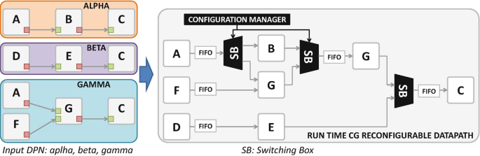

  

  Dataflow to CG reconfigurable substrate [46]

  Fig. 21

  

  Design environment for RVC-CAL compliant CG reconfigurable architectures [58]

• Xronos [7]—capable of providing High Level Synthesis (see Sect. 4.2) from CAL to RTL of each single actor of the given input DPN

• TURNUS [14]—capable of optimizing the system, by means of high-level profiling, to provide the optimal Fifo sizing (in the multi-dataflow case worst case sizing is assigned).

RVC-CAL compliant reconfigurable architectures, assembled as in [58], can be used as the CG reconfigurable processing core of a co-processing unit, as the one presented in Fig. 21 [57].

A DPM-based technique has been used also in a recent work of Edwards et al. [19]. They use the concept of compositional hardware circuits and exploit Kahn Networks to merge and implement in hardware different dataflow networks (Fig. 22).

Fig. 22

Multi-Dataflow Composer (MDC) based reconfigurable co-processor [57]

4.1.2 Coarse-Grained and Runtime Reconfigurable Arrays

Another type of coarse-grain reconfigurable architecture combines a host processor controller with an array of PEs. These PEs, which are typically small and simple like ALUs, are connected together in the array with some local memories. CG reconfigurable arrays are commonly used for efficient implementations of streaming systems [1, 18, 41]. These architectures often exploit imperative programming approaches to map and control the flow of data. The examples hereafter demonstrate how dataflow models can be exploited for the same purposes.

WaveScalar, presented by Swanson et al. in [61], is a dataflow-based reconfigurable architecture that contains a pool of PEs, to which are dynamically assigned instructions: the WaveCache loads instructions from memory and assigns them to PEs for execution. While instruction scheduling is dynamic and out-of-order, the reference application is described as a dataflow graph. Basically, the WaveScalar compiler translates the input imperative programs into a dataflow description, used as the target code. WaveScalar does not implement dataflow-driven reconfiguration, but it is certainly one of the first attempts to combine dataflow models with the CG reconfigurable paradigm.

Galanis et al. have exploited a dataflow-based approach to map different functionalities over the proposed reconfigurable computing array in [23]. In their work the host processor is connected to a co-processing unit, implemented by means of a reconfigurable datapath, where: (1) PEs are an ALU and a multiplier that can take operands from other nodes or from a register bank; and (2) the interconnection among PEs is a full crossbar (or a fat-tree network if scalability issues may arise). Sub-graphs of the parts of the application to be accelerated are mapped over the reconfigurable datapath and the control is generated by an embedded FPGA, which support the overall control flow.

Niedermeier et al. [45], targeting streaming applications, exploited dataflow principles for controlling the flow of data and configuring PEs of their CG architecture. In particular, they configure each PE, including memory blocks, by means of a finite state machine, whose stages are defined as dataflow actors with input and output token patterns. Digital Signal Processing (DSP) applications are particularly suitable to be implemented using such an approach.

Huang et al. [30] adopted dataflow-based control in order to manage complex scheduling situations throughout the propagation of control tokens along with the data to be processed. Such a self control strategy allows to relax mapping and management issues, leveraging on a distributed approach and on a dynamic dataflow control, getting rid of static scheduling. In this way, complex scheduling situations due to latency variations (e.g. when a memory access occurs) are handled transparently with token propagation.

4.2 Fine-Grained Dataflow-Driven Reconfiguration

Bit-level reconfigurability, traditionally required designers to have a deep knowledge of the hardware design flow and hardware description languages. In the last few years, High Level Synthesis (HLS) approaches became popular; they are meant to speed up both hardware and software design process [42]. In particular, from the hardware perspective, one of their advantages is relieving designers from the definition of the RTL description of the system and its components.

A popular commercial HLS synthesizer is Vivado³ from Xilinx, which accelerates IP creation by enabling C, C++ and System C specifications to be directly implemented into Xilinx programmable devices without the need to manually create the RTL description. Similarly, but based on dataflow approaches, Xronos [7] and the Caph compiler [59] are meant to provide dataflow-to-hardware generation. Xronos, which has been developed within RVC-CAL context where dataflow networks expressed using the CAL language based on the DPN MoC, is an evolution of the CAL2HDL framework and the work done in [56]. One of the limitation of Xronos is that it generates a target dependent descriptions implementable only on Xilinx FPGA boards. This limitation is not true for the Caph approach that provides target independent RTL descriptions of dataflow compliant systems, which can be implemented both on ASIC and on FPGA.

Dynamic partial reconfiguration (DPR)⁴ is defined as the ability to modify, at runtime and while the system is executing, blocks/slots of logic by downloading partial bit files. The remaining logic, i.e. those slots where reconfiguration is not applied, keeps running its execution without any interruption. As depicted in Fig. 23, DSP applications may take advantage of DPR, changing tasks in the pipeline while keeping the overall system functional. In this context, the dataflow paradigm is used to address the problem of ensuring that reconfiguration is performed at a convenient time, minimizing its impact on execution latency and memory footprint. By capturing, at compile-time, the application execution in terms of actors exchanging tokens along communications edges, dataflow networks provide a clear definition of dependences. On top of that, their predictability property, enforced by the semantics and execution rules (see Sect. 2.1), can be exploited to manage in advance slots reconfiguration order. In particular, Piat et al. in [53] extended static dataflow description with additional properties to provide compile-time analysis of the DPR influence on the system, to be able to assess early in the design stage DPR time slots and memory requirements. To manage network based reconfiguration, the Parameterized SDFPSDF MoC is adopted, since it is capable of representing dynamic behaviors at network level. Network parameters impact on scheduling/partitioning and memory footprint changes and, therefore, perfectly matches the DPR needs that requires:

• To evaluate buffering requirements on DPR actor inputs—all the incoming edges of the DPR actor are analyzed and the memory cost of the input path is evaluated.

  Fig. 23

  

  Spatial and temporal partitioning of an application in a FPGA exploiting DPR [53]

• To manage slots reconfiguration—a dedicated DPR layer is modelled aside the basic dataflow schedule to represent the reconfiguration instant for each DPR actor, either based on user defined reconfiguration scheme or on network tokens in the case of PSDF model.

In conclusion, as described in this Sect. 4, dataflow specifications may facilitate both mapping and synthesis of coarse and fine grained reconfigurable computing infrastructure to be used in the signal processing domain.

References

Advanced Computer Architecture Group - University of California: Morphosys research project. http://gram.eng.uci.edu/morphosys/
Altera: Increasing Design Functionality with Partial and Dynamic Reconfiguration in 28-nm FPGAs (2010)
Ansaloni, G., Tanimura, K., Pozzi, L., Dutt, N.: Integrated kernel partitioning and scheduling for coarse-grained reconfigurable arrays. IEEE Trans. on CAD of Integrated Circuits and Systems 31(12), 1803–1816 (2012). http://dx.doi.org/10.1109/TCAD.2012.2209886
Battiti, R., Protasi, M.: Reactive local search for the maximum clique problem 1. Algorithmica 29(4), 610–637 (2001)
Beaumin, C., Sentieys, O., Casseau, E., Carer, A.: A coarse-grain reconfigurable hardware architecture for rvc-cal-based design. In: Design and Architectures for Signal and Image Processing (DASIP), 2010 Conference on, pp. 152–159 (2010). https://doi.org/10.1109/DASIP.2010.5706259
Bebelis, V., Fradet, P., Girault, A., Lavigueur, B.: Bpdf: A statically analyzable dataflow model with integer and boolean parameters. In: Proceedings of the Eleventh ACM International Conference on Embedded Software, p. 3. IEEE Press (2013)
Bezati, E., Mattavelli, M., Janneck, J.: High-Level Synthesis of Dataflow Programs for Signal Processing Systems. In: 8th International Symposium on Image and Signal Processing and Analysis (ISPA 2013) (2013)
Bhattacharya, B., Bhattacharyya, S.: Parameterized dataflow modeling for dsp systems. Signal Processing, IEEE Transactions on (2001). https://doi.org/10.1109/78.950795
Bhattacharya, B., Bhattacharyya, S.S.: Quasi-static scheduling of reconfigurable dataflow graphs for dsp systems. In: Proceedings 11th International Workshop on Rapid System Prototyping. RSP 2000. Shortening the Path from Specification to Prototype (Cat. No.PR00668), pp. 84–89 (2000). https://doi.org/10.1109/IWRSP.2000.855200
Bhattacharyya, S.S., Eker, J., Janneck, J.W., Lucarz, C., Mattavelli, M., Raulet, M.: Overview of the mpeg reconfigurable video coding framework. Journal of Signal Processing Systems 63(2), 251–263 (2011)
Bouakaz, A., Fradet, P., Girault, A.: A survey of parametric dataflow models of computation. ACM Trans. Des. Autom. Electron. Syst. 22(2), 38:1–38:25 (2017). https://doi.org/10.1145/2999539. http://doi.acm.org.rproxy.insa-rennes.fr/10.1145/2999539
Boutellier, J., Lucarz, C., Lafond, S., Gomez, V.M., Mattavelli, M.: Quasi-static scheduling of cal actor networks for reconfigurable video coding. Journal of Signal Processing Systems 63(2), 191–202 (2011). http://dx.doi.org/10.1007/s11265-009-0389-5
Boutellier, J., Sadhanala, V., Lucarz, C., Brisk, P., Mattavelli, M.: Scheduling of dataflow models within the reconfigurable video coding framework. In: 2008 IEEE Workshop on Signal Processing Systems, pp. 182–187 (2008). https://doi.org/10.1109/SIPS.2008.4671759
Casale-Brunet, S., Bezati, E., Mattavelli, M., Canale, M., Janneck, J.W.: Execution trace graph analysis of dataflow programs: Bounded buffer scheduling and deadlock recovery using model predictive control. In: Design and Architectures for Signal and Image Processing (DASIP), 2014 Conference on, pp. 1–6 (2014). https://doi.org/10.1109/DASIP.2014.7115623
Compton, K., Hauck, S.: Reconfigurable computing: A survey of systems and software. ACM Comput. Surv. 34(2), 171–210 (2002). http://doi.acm.org/10.1145/508352.508353
Dardaillon, M., Marquet, K., Risset, T., Martin, J., Charles, H.P.: A new compilation flow for software-defined radio applications on heterogeneous mpsocs. ACM Transactions on Architecture and Code Optimization (TACO) 13(2), 19 (2016)
Desnos, K., Pelcat, M., Nezan, J.F., Bhattacharyya, S.S., Aridhi, S.: Pimm: Parameterized and interfaced dataflow meta-model for mpsocs runtime reconfiguration. In: Embedded Computer Systems: Architectures, Modeling, and Simulation (SAMOS XIII), 2013 International Conference on, pp. 41–48. IEEE (2013)
Dongwook Lee Manhwee Jo, K.H.K.C.: FloRA: Coarse-grained reconfigurable architecture with floating-point operation capability. In: International Conference on Field-Programmable Technology (2009)
Edwards, S.A., Townsend, R., Kim, M.A.: Compositional dataflow circuits. In: Proceedings of the 15th ACM-IEEE International Conference on Formal Methods and Models for System Design, MEMOCODE 2017, Vienna, Austria, September 29 - October 02, 2017, pp. 175–184 (2017). http://doi.acm.org/10.1145/3127041.3127055
Ersfolk, J., Roquier, G., Jokhio, F., Lilius, J., Mattavelli, M.: Scheduling of dynamic dataflow programs with model checking. In: Signal Processing Systems (SiPS), 2011 IEEE Workshop on, pp. 37–42. IEEE (2011)
Ersfolk, J., Roquier, G., Lilius, J., Mattavelli, M.: Modeling control tokens for composition of cal actors. In: Design and Architectures for Signal and Image Processing (DASIP), 2013 Conference on, pp. 71–78 (2013)
Fradet, P., Girault, A., Poplavko, P.: Spdf: A schedulable parametric data-flow moc. In: 2012 Design, Automation & Test in Europe Conference & Exhibition (DATE), pp. 769–774. IEEE (2012)
Galanis, M.D., Dimitroulakos, G., Tragoudas, S., Goutis, C.E.: Speedups in embedded systems with a high-performance coprocessor datapath. ACM Trans. Design Autom. Electr. Syst. 12(3), 35:1–35:22 (2007). http://doi.acm.org/10.1145/1255456.1255472
Gorin, J., Wipliez, M., Prêteux, F., Raulet, M.: Llvm-based and scalable mpeg-rvc decoder. Journal of Real-Time Image Processing 6(1), 59–70 (2011)
Goubier, T., Sirdey, R., Louise, S., David, V.: σc: A programming model and language for embedded manycores. In: International Conference on Algorithms and Architectures for Parallel Processing, pp. 385–394. Springer (2011)
Ha, S., Oh, H.: Decidable signal processing dataflow graphs. In: S.S. Bhattacharyya, E.F. Deprettere, R. Leupers, J. Takala (eds.) Handbook of Signal Processing Systems, third edn. Springer (2018)
Hartenstein, R.W.: Coarse grain reconfigurable architecture (embedded tutorial). In: Proceedings of ASP-DAC 2001, Asia and South Pacific Design Automation Conference 2001, January 30-February 2, 2001, Yokohama, Japan, pp. 564–570 (2001). http://doi.acm.org/10.1145/370155.370535
Heulot, J., Boutellier, J., Pelcat, M., Nezan, J.F., Aridhi, S.: Applying the adaptive hybrid flow-shop scheduling method to schedule a 3gpp lte physical layer algorithm onto many-core digital signal processors. In: 2013 NASA/ESA Conference on Adaptive Hardware and Systems (AHS-2013), pp. 123–129 (2013). https://doi.org/10.1109/AHS.2013.6604235
Heulot, J., Pelcat, M., Desnos, K., Nezan, J.F., Aridhi, S.: Spider: A synchronous parameterized and interfaced dataflow-based rtos for multicore dsps. In: 2014 6th European Embedded Design in Education and Research Conference (EDERC), pp. 167–171 (2014). https://doi.org/10.1109/EDERC.2014.6924381
Huang, Y., Ienne, P., Temam, O., Chen, Y., Wu, C.: Elastic cgras. In: Proceedings of the ACM/SIGDA International Symposium on Field Programmable Gate Arrays, FPGA ’13, pp. 171–180. ACM, New York, NY, USA (2013). http://doi.acm.org/10.1145/2435264.2435296
Huang, Z., Malik, S.: Managing dynamic reconfiguration overhead in systems-on-a-chip design using reconfigurable datapaths and optimized interconnection networks. In: Proceedings of the Conference on Design, Automation and Test in Europe, DATE ’01, pp. 735–. IEEE Press, Piscataway, NJ, USA (2001). http://dl.acm.org/citation.cfm?id=367072.367934
Kee, H., Shen, C.C., Bhattacharyya, S.S., Wong, I., Rao, Y., Kornerup, J.: Mapping parameterized cyclo-static dataflow graphs onto configurable hardware. Journal of Signal Processing Systems (2012)
Keinert, J., Deprettere, E.F.: Multidimensional dataflow graphs. In: S.S. Bhattacharyya, E.F. Deprettere, R. Leupers, J. Takala (eds.) Handbook of Signal Processing Systems, second edn. Springer (2013)
Kenneth Pocek Russell Tessier, A.D.: Birth and adolescence of reconfigurable computing: a survey of the first 20 years of field-programmable custom computing machines. Field-Programmable Custom Computing Machines, Annual IEEE Symposium on 00(undefined), 1–17 (2013). http://doi.ieeecomputersociety.org/10.1109/FPGA.2013.6882273
Ko, M.Y., Zissulescu, C., Puthenpurayil, S., Bhattacharyya, S.S., Kienhuis, B., Deprettere, E.F.: Parameterized looped schedules for compact representation of execution sequences in dsp hardware and software implementation. IEEE Transactions on Signal Processing 55(6), 3126–3138 (2007)
Lattner, C.: Llvm and clang: Advancing compiler technology. Proc. of FOSDEM (2011)
Lee, E.A., Ha, S.: Scheduling strategies for multiprocessor real-time dsp. In: Global Telecommunications Conference and Exhibition’Communications Technology for the 1990s and Beyond’(GLOBECOM), 1989. IEEE, pp. 1279–1283. IEEE (1989)
Lee, E.A., Parks, T.M.: Dataflow process networks. Proceedings of the IEEE 83(5), 773–801 (1995)
Leupers, R., Aguilar, M.A., Castrillon, J., Sheng, W.: Software compilation techniques for heterogeneous embedded multi-core systems. In: S.S. Bhattacharyya, E.F. Deprettere, R. Leupers, J. Takala (eds.) Handbook of Signal Processing Systems, third edn. Springer (2018)
Lin, S., Wang, L.H., Vosoughi, A., Cavallaro, J.R., Juntti, M., Boutellier, J., Silvén, O., Valkama, M., Bhattacharyya, S.S.: Parameterized sets of dataflow modes and their application to implementation of cognitive radio systems. Journal of Signal Processing Systems 80(1), 3–18 (2015). http://dx.doi.org/10.1007/s11265-014-0938-4
Liu, L., Wang, D., Zhu, M., Wang, Y., Yin, S., Cao, P., Yang, J., Wei, S.: An energy-efficient coarse-grained reconfigurable processing unit for multiple-standard video decoding. IEEE Trans. Multimedia 17(10), 1706–1720 (2015)
Martin, G., Smith, G.: High-level synthesis: Past, present, and future. IEEE Design & Test of Computers 26(4), 18–25 (2009). http://dx.doi.org/10.1109/MDT.2009.83
Moreano, N., Araujo, G., Huang, Z., Malik, S.: Datapath merging and interconnection sharing for reconfigurable architectures. In: System Synthesis, 2002. 15th International Symposium on, pp. 38–43 (2002)
Neuendorffer, S., Lee, E.: Hierarchical reconfiguration of dataflow models. In: MEMOCODE (2004). https://doi.org/10.1109/MEMCOD.2004.1459852
Niedermeier, A., Kuper, J., Smit, G.: Dataflow-based reconfigurable architecture for streaming applications. In: System on Chip (SoC), 2012 International Symposium on, pp. 1–4 (2012). https://doi.org/10.1109/ISSoC.2012.6376365
Palumbo, F., Carta, N., Pani, D., Meloni, P., Raffo, L.: The multi-dataflow composer tool: generation of on-the-fly reconfigurable platforms. Journal of real-time image processing 9(1), 233–249 (2014)
Palumbo, F., Sau, C., Evangelista, D., Meloni, P., Pelcat, M., Raffo, L.: Runtime energy versus quality tuning in motion compensation filters for hevc. IFAC-PapersOnLine 49(25), 145–152 (2016)
Palumbo, F., Sau, C., Fanni, T., Meloni, P., Raffo, L.: Dataflow-based design of coarse-grained reconfigurable platforms. In: Signal Processing Systems (SiPS), 2016 IEEE International Workshop on, pp. 127–129. IEEE (2016)
Pelcat, M., Aridhi, S., Piat, J., Nezan, J.F.: Physical layer multi-core prototyping: a dataflow-based approach for LTE eNodeB, vol. 171. Springer Science & Business Media (2012)
Pelcat, M., Desnos, K., Heulot, J., Guy, C., Nezan, J.F., Aridhi, S.: Preesm: A dataflow-based rapid prototyping framework for simplifying multicore dsp programming. In: Education and Research Conference (EDERC), 2014 6th European Embedded Design in, pp. 36–40 (2014). https://doi.org/10.1109/EDERC.2014.6924354
Piat, J., Bhattacharyya, S., Raulet, M.: Interface-based hierarchy for synchronous data-flow graphs. In: SiPS Proceedings (2009). https://doi.org/10.1109/SIPS.2009.5336240
Piat, J., Crenne, J.: Modeling dynamic partial reconfiguration in the dataflow paradigm. In: 2014 IEEE Workshop on Signal Processing Systems (SiPS), pp. 1–6. IEEE (2014)
Plishker, W., Sane, N., Bhattacharyya, S.S.: Mode grouping for more effective generalized scheduling of dynamic dataflow applications. In: Proceedings of the 46th Annual Design Automation Conference, pp. 923–926. ACM (2009)
Ren, R., Juarez, E., Sanz, C., Raulet, M., Pescador, F.: Energy-aware decoder management: a case study on rvc-cal specification based on just-in-time adaptive decoder engine. IEEE Transactions on Consumer Electronics 60(3), 499–507 (2014). https://doi.org/10.1109/TCE.2014.6937336
Roquier, G., Bezati, E., Thavot, R., Mattavelli, M.: Hardware/software co-design of dataflow programs for reconfigurable hardware and multi-core platforms. In: 2011 Conference on Design and Architectures for Signal and Image Processing, DASIP 2011, Tampere, Finland, November 2–4, 2011, pp. 171–177 (2011). http://dx.doi.org/10.1109/DASIP.2011.6136875
Sau, C., Fanni, L., Meloni, P., Raffo, L., Palumbo, F.: Reconfigurable coprocessors synthesis in the mpeg-rvc domain. In: ReConFigurable Computing and FPGAs (ReConFig), 2015 International Conference on, pp. 1–8. IEEE (2015)
Sau, C., Meloni, P., Raffo, L., Palumbo, F., Bezati, E., Casale-Brunet, S., Mattavelli, M.: Automated design flow for multi-functional dataflow-based platforms. Journal of Signal Processing Systems 85(1), 143–165 (2016)
Sérot, J., Berry, F.: High-level dataflow programming for reconfigurable computing. In: Proceedings of the 2014 International Symposium on Computer Architecture and High Performance Computing Workshop, SBAC-PADW ’14, pp. 72–77. IEEE Computer Society, Washington, DC, USA (2014). http://dx.doi.org/10.1109/SBAC-PADW.2014.18
Souza, C.C.d., Lima, A.M., Araujo, G., Moreano, N.B.: The datapath merging problem in reconfigurable systems: Complexity, dual bounds and heuristic evaluation. J. Exp. Algorithmics 10 (2005). http://doi.acm.org/10.1145/1064546.1180613
Swanson, S., Schwerin, A., Mercaldi, M., Petersen, A., Putnam, A., Michelson, K., Oskin, M., Eggers, S.J.: The wavescalar architecture. ACM Trans. Comput. Syst. 25(2), 4:1–4:54 (2007). http://doi.acm.org/10.1145/1233307.1233308
Tessier, R., Burleson, W.: Reconfigurable computing for digital signal processing: A survey. VLSI Signal Processing 28(1–2), 7–27 (2001). http://dx.doi.org/10.1023/A:1008155020711
Tessier, R., Pocek, K.L., DeHon, A.: Reconfigurable computing architectures. Proceedings of the IEEE 103(3), 332–354 (2015). http://dx.doi.org/10.1109/JPROC.2014.2386883
Theelen, B.D., Deprettere, E.F., Bhattacharyya, S.S.: Dynamic dataflow graphs. In: S.S. Bhattacharyya, E.F. Deprettere, R. Leupers, J. Takala (eds.) Handbook of Signal Processing Systems, third edn. Springer (2018)
Wijtvliet, M., Waeijen, L., Corporaal, H.: Coarse grained reconfigurable architectures in the past 25 years: Overview and classification. In: International Conference on Embedded Computer Systems: Architectures, Modeling and Simulation, SAMOS 2016, Agios Konstantinos, Samos Island, Greece, July 17–21, 2016, pp. 235–244 (2016). http://dx.doi.org/10.1109/SAMOS.2016.7818353
Xilinx: Partial Reconfiguration User Guide (2012)
Yviquel, H., Casseau, E., Wipliez, M., Gorin, J., Raulet, M.: Classification-based optimization of dynamic dataflow programs. In: Advancing Embedded Systems and Real-Time Communications with Emerging Technologies, pp. 282–301. IGI Global (2014)
Yviquel, H., Sanchez, A., Mickaël, R., Casseau, E.: Technical Report: Multicore Runtime for Dynamic Dataflow Video Decoders. Technical report, IETR/INSA Rennes; IRISA, Inria Rennes (2017). https://hal.archives-ouvertes.fr/hal-01503378
Acknowledgements
This work was partially supported by the CERBERO (Cross-layer modEl-based fRamework for multi-oBjective dEsign of Reconfigurable systems in unceRtain hybRid envirOnments) Horizon 2020 Project, funded by the European Union Commission under Grant 732105.
Author information
Authors and Affiliations
Corresponding author
Editor information
Editors and Affiliations
Rights and permissions
Copyright information
© 2019 Springer International Publishing AG, part of Springer Nature
About this chapter
Cite this chapter
Desnos, K., Palumbo, F. (2019). Dataflow Modeling for Reconfigurable Signal Processing Systems. In: Bhattacharyya, S., Deprettere, E., Leupers, R., Takala, J. (eds) Handbook of Signal Processing Systems. Springer, Cham. https://doi.org/10.1007/978-3-319-91734-4_22
Download citation
DOI: https://doi.org/10.1007/978-3-319-91734-4_22
Published:
Publisher Name: Springer, Cham
Print ISBN: 978-3-319-91733-7
Online ISBN: 978-3-319-91734-4
eBook Packages: EngineeringEngineering (R0)