Computer Vision-Based Method for Automatic Detection of Crop Rows in Potato Fields

Abstract

This work presents an adaptation and validation of a method for automatic crop row detection from images captured in potato fields (Solanum tuberosum) for initial growth stages based on the micro-ROI concept. The crop row detection is a crucial aspect for autonomous guidance of agricultural vehicles and site-specific treatments application. The images were obtained using a color camera installed in the front of a tractor under perspective projection. There are some issues that can affect the quality of the images and the detection procedure, among them: uncontrolled illumination in outdoor agricultural environments, different plant densities, presence of weeds and gaps in the crop rows. The adapted approach was designed to address these adverse situations and it consists of three linked phases. The main contribution is the ability to detect straight and curved crop rows in potato crops. The performance was quantitatively compared against two existing methods, achieving acceptable results in terms of accuracy and processing time.

1 Introduction

Artificial vision systems installed on autonomous tractors are useful tools for performing crop rows detection [1] as well as site-specific treatments application [2], including the removal of weeds that are located outside the crop rows. In such type of vehicles, the navigation is mainly based on Global Positioning Systems (GPS) [3]. However, when small deviations occur in navigation, the detection of crop rows becomes crucial to accomplish a correction process [4] in site. Agricultural environments are affected by several adverse situations that influence the crop rows detection process, such as: uncontrolled lighting in outdoor agricultural environments; discontinuities in crop rows due to defects in sowing or germination; weeds with green colors similar to crops; variety of heights and volumes of plants due to the growth stages; curved crop rows that may be created in certain irregular and/or rugged fields.

Several approaches based on image analyses (e.g. Hough transform, linear regression, horizontal stripes, region analysis, filtering, stereo vision, green pixel accumulation) have been mainly conducted for detection of straight crop rows [1, 5, 6] and to a lesser extent for curved crop rows [7, 8]. Indeed, some researches have opted by combining many approaches with a prior knowledge included through different constraints in order to decrease the algorithmic complexity, enabling them for real time applications. Based on the trends and studies reported in recent literature, this work aims to adapt and validate a computer vision method based on micro-ROI [9] for automatic detection of crop rows in potato fields, superchola variety (Solanum tuberosum), at initial stages of growth (≤40 days). The adaptation of the original method (validated in maize fields) to another type of crop (potato fields) with other phenological and physiological characteristics constitutes the main contribution of this research.

2 Materials and Methods

2.1 Image Set

Images were acquired in a potato field from Ibarra-Ecuador during January and February 2017. The field is non-regular, exhibiting slopes up to 8°. Images were acquired under different lighting conditions and growth stages (≤40 days), as shown in Fig. 1. Some instances of images are: (a) plants of different sizes in a sunny day, (b) low weed presence in a dark day, and (c) discontinuities into crop rows in a clear day. The crop rows were spaced, an average, 0.90 m and curved furrows were oriented to the left. A total of 320 images were randomly selected for experimentation.

Fig. 1.

Instances of the image set processed by the adapted approach in potato fields, namely: (a) plants of different sizes in a sunny day, (b) low weed presence in a dark day, and (c) discontinuities into crop rows in a clear day.

The images were obtained under perspective projection with a goPro Hero 3+ Black Edition color camera with a focal length of 3 mm. The camera was installed on the front of a New Holland TD90 tractor and located at a height between 1.80 m and 2 m from the ground with an inclination between 40° and 50°, as shown in Fig. 2.

Fig. 2.

Acquisition process: (a) Vision system installed on tractor; (b) Location of the region of interest (ROI) into an image

The images were stored in a JPG format with a resolution of 3000 × 2250 pixels (7 Mpx). The size and location of the region of interest (ROI) were established to detect 4 crop rows [1], containing sufficient resolution for detecting objects of interest [10]. The length of the ROI was set to 5 m (in the potato field) and the ROI have a resolution of 2000 × 650 pixels (width × length) in the projected 2D image (Fig. 2b). The images were processed using Matlab R2015a software [11] executing on an Intel Core i7 2.0 GHz processor (4th generation), 8 GB RAM and Windows 8.1 Pro (64-bit).

2.2 Outline of the Method

Adapted approach is based on [9], which was validated in maize fields, and consists of three stages: (i) image segmentation, (ii) starting point’s identification, and (iii) crop rows detection.

2.2.1 Image Segmentation: It stage consists of 4 steps as explained below:

• (a) ROI identification: As previously mentioned (regarding Fig. 2b), the ROI was selected containing 4 crop rows with a suitable resolution.

• (b) Identification of greens: Given the evidence of its good results reported in literature, the index ExG (Excess Green) described in [12] was used. Its standard formulation is given in Eq. (1). Figure 3(a) shows the ROI within a grayscale image where ExG index was applied.

  Fig. 3.

  

  Examples of ROI images: (a) ExG; (b) double thresholding; and (c) morphological operations.

  $$ ExG = 2g - r - b $$

  (1)

• (c) Double thresholding: A first thresholding process, based on [13], was applied to separate vegetation (crop and weed) and soil. Then, a second thresholding was applied to the vegetation pixels to separate the crop and weeds. Figure 3(b) shows the ROI as a binary image containing the potato crop in white pixels, while soil in black pixels.

• (d) Morphological operations: morphological opening [14] and 5 × 5 majority filter were applied to remove isolated pixels, and obtaining cleaner binary images for further processing (Fig. 3c).

2.2.2 Starting Point’s Identification: This stage aims to locate the starting points on the ROI, which are the basis for searching the crop rows. It works as follows:

• (a) The ROI is divided into two same-sized horizontal strips: lower and higher (see Fig. 4).

  Fig. 4.

  

  Location of 4 stating points in the lower ROI strip.

• (b) The Hough transform (HT) [15] is applied in the lower ROI strip to identify linear segments of white pixels. To do so, some constraints are assumed by a priori knowledge in order to decrease the computational complexity, such as the orientation of lines between −45° and 45°, four peaks in the Hough polar space (rho, theta) with a resolution of 1 pixel and 1°, respectively.

• (c) Four peaks (lines) are identified in the Hough polar space, which in turn determine 4 parameters m (slope) and b (intercept) associated with the 4 linear segments. The points of intersection between the lines detected with TH and the lower edge of ROI determine the initial 4 points, as can be observed in Fig. 4 (red points). Likewise, the slope of each linear segment indicates the direction to start the search of the plants and then the crop rows within the ROI.

2.2.3 Crop Rows Detection: This stage encompasses three processes: (a) extraction of candidate points, (b) regression analysis and (c) crop rows selection

• (a) Extraction of candidate points: The ROI (depicted in Fig. 3c) is divided into 10 same-sized horizontal substrips (see Fig. 5), unlike the 12 substrips of the original method [9]. This number was established after trial and error tests with the curvature of the crop rows in the images considered for experiments. Thus, the lower and upper ROI strips contain four and six substrips, respectively. The curved lines appear more pronounced at the top of the ROI because of the perspective projection, so the number of substrips (six) enables to capture such variability (curvature) more precisely.

  Fig. 5.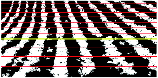

  

  The ROI is divided into ten substrips of equal size. Four in the lower ROI and six in the upper strip.

Crop rows are extracted sequentially from left to right, exploring the ten substrips vertically from bottom to top of the ROI, based on the concept of micro-ROIs, starting from the associated starting point (Fig. 4) and with the slope of the straight line estimated with TH, used as a guidance (direction). Consequently, a micro-ROI determines a small rectangular region (window). The height of each micro-ROI is the same as that of the corresponding substrip, while the width varies in each substrip due to perspective projection, being initially fixed at 160 pixels (0.30 m in the ROI base), gradually decreasing at the rate of 6% as measured that ascends by the substrips. The objective of each micro-ROI is to include the maximum number of potato plants, leaving mostly weeds that are located in the inter-row spaces. Each micro-ROI is defined by four parameters [x, y, width, height], where the point (x, y) represents the upper left corner. The parameters y, width, and height are beforehand known once the horizontal substrips are established (Fig. 5), while x is unknown and is obtained dynamically for each substrip as follows:

• 1. The first micro-ROI is located with the base centered at the first initial point (Fig. 4). The geometric center of the micro-ROI is calculated [16], obtaining P1 $\left( {x_{1} , y_{1} } \right)$, Fig. 6 (yellow cross). This expression is less sensitive to noise and minimizes the effects of isolated pixels belonging to the weeds located in the space between cultivation lines.

  Fig. 6.

  

  Location of the first micro-ROI in the first substrip, where the red cross is the center of the micro-ROI at the base and the yellow cross is the centroid P₁.

• 2. Following the estimated line of reference with TH (Fig. 4), three additional micro-ROIs are placed with the bases centered at the points of intersection between the reference line (HT) and the lower edges of the substrips, Fig. 7.

  Fig. 7.

  

  Location of the fourth micro-ROI, where the yellow cross is the centroid P₄.

In the upper strip of the ROI, which contains six substrips (Fig. 5), each micro-ROI is placed centered on the point of intersection between the lower edge of the corresponding substrip and the estimated straight line with the four previously calculated centroids, i.e. with the points based on record that define the trend of the crop rows. The straight line is adjusted using least squares linear regression as follows:

• 3. The fifth micro-ROI, Fig. 8, is located considering the last four centroids (P₁, P₂, P₃, P₄), from which a straight line is fitted, obtaining the corresponding slope m_1,2,3,4. The intersection point (red cross) in the next substrip (fifth) is obtained using the last centroid P4 and the slope m_1,2,3,4.

  Fig. 8.

  

  Location of the fifth micro-ROI, where the yellow cross is the centroid P₅.

• 4. The centroid P₅ (yellow cross) is calculated within the micro-ROI as before.

• 5. Steps 3 and 4 apply to other micro-ROIs within the upper strip of the ROI, Fig. 9. For example, if centroid P₁₀, is considered, the line is adjusted considering the four previous centroids (P₆, P₇, P₈, P₉) with the slope m_6,7,8,9. Thus, the intersection point in the next substrip is obtained using centroid P₉ with slope m_6,7,8,9.

  Fig. 9.

  

  Location of the tenth micro-ROI, where the yellow cross is the centroid P₁₀.

• 6. Once the ten substrips are processed, a set of 10 points distributed along the first crop row is obtained, object of detection.

The complete procedure (steps 1–6) is repeated for other available starting points (Fig. 4). Figure 10 shows the result of this process on the four crop rows. The candidate points obtained constitute the entry for the subsequent regression analysis process.

Fig. 10.

Location of micro-ROIs (blue rectangles) along crop rows that cross the top and bottom edges of the ROI.

• (b) Regression Analysis: With the candidate points obtained in the previous process, polynomials of degree one (straight line) and two (quadratic curve) are adjusted for each crop row using the least squares technique. The coefficients to be estimated for the straight line are the slope (m) and the intercept (b); while for quadratic polynomial are coefficients a, b and c, Eq. (2).

$$ y = mx + b; \quad y = ax^{2} + bx + c. $$

(2)

Figure 11(a) shows the two polynomials (straight and quadratic) obtained for each crop row within the ROI. The least squares technique also provides the norm of residues (R), which is a measure of the quality of the fitting. The smaller the R, the better the adjustment performed. This measurement is used in the following process for the selection of the best lines.

Fig. 11.

Polynomials obtained for each crop row within the ROI. (a) Straight and quadratic lines; (b) selection of lines that fitted better.

• (c) Crop row selection: The selected polynomial (straight or quadratic) is the one that best fits each crop row based on the norm of residues (R), i.e. the line with the lowest R value, Fig. 11b. As a final result, the method detects 4 crop rows (curves and/or straight) and mathematically modeled (Eq. 2).

The robustness of the adapted method is complemented by three verification procedures: (i) the number of lines detected must be equal to four; (ii) the separation of crop rows at the base of the ROI does not exceed 600 pixels, which was set by experimentation; (iii) there is no intersection between the crop rows detected within the ROI. In case of any anomaly, the image is rejected and next one is processed.

Regarding the crop row curvature, the method was designed for curvatures toward left. However, when the curvature is oriented to the right (Fig. 12a), the method works by applying to the ROI a vertical specular reflection operation (Fig. 12b) and horizontal translational operations on the points identified along the crop rows (Fig. 10) [7]. In this way, the algorithm can work with crop rows with curvatures oriented left or right, but not both simultaneously.

Fig. 12.

(a) ROI with crop rows oriented to the right in potato crops. (b) ROI after applying a vertical specular reflection operation.

3 Results and Discussion

The performance of the adapted approach, here-named DBMR (Detection Based on Micro-ROI) -maintaining the original nomenclature from [9]- was quantitatively compared against 2 existing methods, which are capable of detecting both straight and curved crop rows: (i) Template matching with Global Energy Minimization (TMGEM) in order to detect regular patterns and determine an optimal crop model using dynamic programming [8]; (ii) Detection for accumulation of green pixels (DAGP) for exploring candidate alignments of green pixels that define straight and quadratic crop rows [7]. The two existing methods were selected for comparison purposes because, as far as is known, there are no other methods available with such capabilities for detecting straight and curved crop rows.

The CRDA measure (Crop Row Detection Accuracy), proposed in [8], was used to evaluate the performance of the methods, whose value is between [0, 1], where the best score is the unit. CRDA measures the coincidence between the horizontal coordinates of each crop row, obtained by each method under evaluation (DBMR, TMGEM, and DAGP) and the corresponding values of the ground truth. The ground truth was manually created by an expert based on visual observation, where at least five points were selected on each crop row and squared curves were fitted using the curve fitting toolbox incorporated into Matlab [11]. In total, 320 images were randomly selected, containing straight and curved crop rows, spaced both regularly and irregularly. Irregular spacing of crop rows usually occurs when the tractor crosses the crop several times, displacing soil in each pass (as can be noticed from Fig. 13d).

Fig. 13.

Examples of the set of images in potato fields containing straight and curved crop rows detected by the DBMR adapted method.

Figure 13 shows some examples of the processed images by the DBMR adapted method with the respective CDRA metrics. In Fig. 13(a) and (b) with straight crop rows; Fig. 13(c) to (f) with curved crop rows; (g) and (h) a mixture of curved (red) and straight (blue) crop rows.

As can be noted in Fig. 13(a) and (f), some crop rows may contain discontinuities caused by defects in planting or germination. In this study, the gaps do not exceed 1.20 m of discontinuity in the same furrow according to the vision system configuration. A longer length may result in a fault in the crop row detection. In addition, weeds are often distributed irregularly into the inter-row spaces, as can be appreciated in Fig. 13(a) and (b). For experimental purposes, the method was tested with a low weed level, i.e. up to 5% of weed cover according to the classification scale proposed in [17]. A higher level of weed may lead to incorrect crop row detection. Both factors, crop row discontinuity and weed level affect the performance of the DBMR adapted method (see Fig. 13a).

Table 1 shows the average percentage detection rate for the 320 analyzed images with curvatures oriented toward left or right. From the results, it can be seen that DBMR exceeds to the two existing methods TMGEM and DAGP in potato crops, which is in agreement with the results reported in [9] in maize crops. The adapted method DBMR fits well to the curvature of potato crop rows using 10 substrips (Fig. 5), unlike the 12 substrips used in [9]. This is due to the fact that the minimum radius of curvature in potato crops was greater than those of the maize crop, which was 19 m.

Table 1. Comparison of the adapted method DBMR against TMGEM and DAGP regarding CRDA measure, whose value is between [0, 1], being the unit the best score.

The DAGP and DBMR methods were implemented in Matlab, while TMGEM in C++. Table 2 shows the average processing time for the complete process of the adapted method DBMR, which was 694 ms, measured in Matlab under an interpreted programming language that is slower than a compiled (e.g. C++). So, the method shows potential for real-time applications, which is an aspect to be studied in further researches. The increase of execution time when running DBMR with respect to that reported in [9] can be attributed to the fact that the potato crop is leafier than maize crop, so it requires the processing of a greater number of pixels during the involved stages (segmentation, identification of starting points, crop row detection).

Table 2. Average execution time in milliseconds (ms) for the three methods: TMGEM, DAGP, and DBMR adapted method.

According to the working conditions of the DBMR adapted method, its application requires that three main input parameters are beforehand known, namely: (i) number of crop rows to be detected, (ii) crop row concavity, and (iii) the intrinsic and extrinsic parameters of the visual system.

Finally, as a future work, following issues are to be considered: (i) the implementation of DBMR using a compiled programming language running on a real-time operating system and platform, following the ideas of the RHEA (2014) project. (ii) The implementation of the DBMR method using parallel programming techniques would be advisable in order to reduce the processing time for real-time application. (iii) Test DBMR method over other crops that are important in the northern region of Ecuador, such as: bean, pea and onion.

4 Conclusions

This work presents an adaptation of a computer vision method, based on micro-ROIs [9], here-called DBMR, for detection of straight and curved crop rows (oriented toward left or right, but not simultaneously) in potato fields, superchola variety (Solanum tuberosum), in initial stages of growth (≤40 days). Adapted approach consists of 3 stages, namely: segmentation, identification of starting points, and crop rows detection. To evaluate the performance of the algorithm, the CRDA measure is used, which reaches 1 as highest score. The DBMR adapted method works well in the presence of low weed levels (CRDA > 0.87) involving processing times less than 694 ms, exhibiting a potential for real-time applications.

References

Gonzalez-de-Santos, P., Ribeiro, A. (eds.): Proceedings of the Second International Conference on Robotics and Associated High-Technologies And Equipment for Agriculture and Forestry: New Trends in Mobile Robotics, Perception and Actuation for Agriculture and Forestry, RHEA (2014)
Gée, C., Bossu, J., Jones, G., Truchetet, F.: Crop/weed discrimination in perspective agronomic images. Comput. Electron. Agric. 60(1), 49–59 (2008)
Emmi, L., Gonzalez-de-Soto, M., Pajares, G., Gonzalez-de-Santos, P.: New trends in robotics for agriculture: integration and assessment of a real fleet of robots. Sci. World J. 2014, 21 pages (2014). Article ID 404059
Rovira-Más, F., Zhang, Q., Reid, J.F., Will, J.D.: Machine vision based automated tractor guidance. Int. J. Smart Eng. Syst. Des. 5(4), 467–480 (2003)
Montalvo, M., Pajares, G., Guerrero, J.M., Romeo, J., Guijarro, M., Ribeiro, A., Cruz, J.M.: Automatic detection of crop rows in maize fields with high weeds pressure. Expert Syst. Appl. 39(15), 11889–11897 (2012)
Guerrero, J.M., Guijarro, M., Montalvo, M., Romeo, J., Emmi, L., Ribeiro, A., Pajares, G.: Automatic expert system based on images for accuracy crop row detection in maize fields. Expert Syst. Appl. 40(2), 656–664 (2013)
García-Santillán, I., Guerrero, J., Montalvo, M., Pajares, G.: Curved and straight crop row detection by accumulation of green pixels from images in maize fields. Precision Agriculture (2017). https://doi.org/10.1007/s11119-016-9494-1
Vidovic, I., Cupec, R., Hocenski, Z.: Crop row detection by global energy minimization. Pattern Recogn. 55, 68–86 (2016)
García-Santillán, I., Montalvo, M., Guerrero, M., Pajares, G.: Automatic detection of curved and straight crop rows from images in maize fields. Biosyst. Eng. 156, 61–79 (2017). https://doi.org/10.1016/j.biosystemseng.2017.01.013
Pajares, G., García-Santillán, I., Campos, Y., Montalvo, M., Guerrero, J.M., Emmi, L., et al.: Machine-vision systems selection for agricultural vehicles: a guide. J. Imag. 2, 34 (2016)
MathWorks, Inc. (2015). http://www.mathworks.com/products/new_products/release2015a.html
Sogaard, H.T., Olsen, H.J.: Determination of crop rows by image analysis without segmentation. Comput. Electron. Agric. 38(2), 141–158 (2003)
Otsu, N.: Threshold selection method from gray-level histograms. IEEE Trans. Syst. Man Cybern. 9(1), 62–66 (1979)
Onyango, C.M., Marchant, J.A.: Segmentation of row crop plants from weeds using colour and morphology. Comput. Electron. Agric. 39(3), 141–155 (2003)
Hough, P.: Method and means for recognizing complex patterns. Patente 3069654 (1962)
Gonzalez, R., Woods, R.: Digital Image Processing, 3rd edn. Pearson/Prentice Hall, Upper Saddle River (2010)
Maltsev, A.I.: Weed Vegetation of the USSR and Measures of its Control. Selkhozizdat, Leningrad-Moscow (1962). (in Russian)
Author information
Authors and Affiliations
Corresponding author
Editor information
Editors and Affiliations
Rights and permissions
Copyright information
© 2018 Springer International Publishing AG
About this paper
Cite this paper
García-Santillán, I., Peluffo-Ordoñez, D., Caranqui, V., Pusdá, M., Garrido, F., Granda, P. (2018). Computer Vision-Based Method for Automatic Detection of Crop Rows in Potato Fields. In: Rocha, Á., Guarda, T. (eds) Proceedings of the International Conference on Information Technology & Systems (ICITS 2018). ICITS 2018. Advances in Intelligent Systems and Computing, vol 721. Springer, Cham. https://doi.org/10.1007/978-3-319-73450-7_34
Download citation
DOI: https://doi.org/10.1007/978-3-319-73450-7_34
Published:
Publisher Name: Springer, Cham
Print ISBN: 978-3-319-73449-1
Online ISBN: 978-3-319-73450-7
eBook Packages: EngineeringEngineering (R0)