
Abstract
The use of PLM tools is widely spread in the aeronautical industry. Although scheduling and line balancing have remained aside these tools for long, they are being developed in the recent years. They need to tackle with complex resource constrained scheduling problems. In this work we present a simulation model we have developed for evaluating the robustness of a baseline scheduling for an aero structure assembly line. To begin with, we have identified and quantified the main causes of the disruptions. Then we have created a discrete event simulation model of the production line to take everything into consideration, and then run several experiments to evaluate different production planning obtained with the different methodologies and the impact of failures in the deliveries of finished products. Also, different scenarios in terms of failure quantity and typology have been studied.
You have full access to this open access chapter, Download conference paper PDF
Keywords
1 Introduction
The use of PLM tools is widely spread in the aeronautical industry. Mas et al. (2015a) provided a detailed review on the impact that PLM tools have had on this industry. They stated it has been a major enabler for shortening development timeframes in spite of the increasing aircraft complexity. According to them, one of the current challenges of PLM tools is to allow the simulation of the whole manufacturing of the aircraft.
During the define phase of an assembly line, the conceptual design is tested against a set of what if scenarios (Mas et al. 2013). Discrete event simulation models can contribute to the evaluation of the expected performance, providing additional information to that on the industrial Digital Mock Up (iDMU) (Mas et al. 2015b). Moreover, although process simulation has been used more often in that early design phase (Jahangirian et al. 2010) it can also provide valuable inputs later in the lifecycle. As stated by Murphy and Perera (2002), it can provide quicker response time for decision making and evaluation of those decisions.
In this work, we have used simulation as part of the scheduling and line balancing system, in order to test the robustness of different production scheduling solutions in a set of what if scenarios. It uses the detailed process definition from the industrial iDMU and, once validated, provides information to the Manufacturing Execution System (MES) see Fig. 1.

Context of the scheduling and line balancing system
The model uses two kinds of inputs: on the one hand, it uses the detailed process definition coming from the previous. On the other, we have worked on the identification and quantification of the main causes of disruptions.
Afterwards, it has been used to run several experiments to evaluate different production schedules and risk avoidance strategies in terms of resource management. For each of them, several scenarios in terms of disruption rates have been studied.
Using this simulation model, it is possible to compare the delivery rate of the finished products. This comparison between different schedules in the face of multiple objectives is not straightforward. For example a production planning that minimizes the number of operators may be less robust to any failure or absence of workers but perform better in terms of work in progress.
We believe that this simulation tool can provide a wider understanding on the assembly line expected behavior. Together with a scheduling tool or on its own it can provide useful information for preventive risk management as it helps to evaluate the results of different production schedules or line designs.
This paper is organized as follows: In the next section, we present a Literature Review. In Sect. 3 we present the Method and briefly discuss its validation. Section 4 is dedicated to the simulation results. Finally, in Sect. 5 we draw the final discussion and future research.
2 Literature Review
Scheduling in the aeronautical industry is a complex resource constrained scheduling problem. For example, in the aero structure part manufacturing it is necessary to schedule within the same assembly line, several parts that share resources, and have different production tasks and times.
This scheduling has been traditionally done by hand, relying on experts’ knowledge. Nowadays, there are mathematical programming tools to do it. However, during the tasks execution there are multiple disruption sources that need to be tackled. There is an interest of defining a robust baseline schedule, defined as a schedule whose performance remains high in the place of disruptions (Leon et al. 1994).
There are different approaches in order to pursue or asses schedule robustness. The three main strategies are reactive scheduling, incorporating uncertainty in the baseline schedule (by means of stochastic, fuzzy or robust scheduling) and sensitivity analysis (Herroelen and Leus 2005). In our case, the mathematical model of the scheduling baseline is already complex and makes it impossible for real life instances to add the complexity of disruptions. Therefore, we have used discrete event simulation in order to provide a sensitivity analysis and evaluate the impact of the different unforeseen events on different production plans.
Discrete event simulation is a form of computer-based modeling that provides an intuitive and flexible approach to representing complex systems. It models the operation of the factory as a sequence of events that occur in a particular part of the time. The state of the system changes only when an event occurs. It has proven a useful technique for manufacturing systems analysis. (Cunha and Mesquita 1996; Kadar et al. 2004). In the case of the aeronautical industry, Scott (1994) provided an early overview of the most relevant aspects for aeronautical assembly line simulations. Most of the later references have dealt with problems related to final assembly lines. Heike et al. (2001) published a case study to compare the use of constant or variable cycle times within a flow shop. Ziarnetzky (2014) used discrete-event simulation for analysing different inventory policies during a station of a final assembly line. It considers supplier and production disruptions. Lu et al. (2012) used simulation to identify bottlenecks and Noack and Rose (2008) proposed simulation optimization for workforce balancing.
Nonetheless, the literature is still surprisingly lacking of contributions discussing the utilization of simulation in the aero structure production. Neither has it been used to test operator management strategies, as is the case of our study. This can serve for a dual purpose: as a support in the design of the aeronautic production line and during the short and long term planning of the aero structure production.
3 Method
The object of our case study is an aero structure assembly line that produces two aero structures (FCA and FCB), each of them in their right hand (RH) and the left hand (LH) version. In all, 4 products are delivered by the line, called: FC-A LH, FC-A RH, FC-B LH and FC-B RH. Each product goes through nine different steps.
The production times per step and product, could be considered constant. At the same time, the problem is that the circumstances for the production change from one week to another. The holidays or programed maintenance are taken in consideration in the baseline schedule, but other disruptions such as break downs, absence of workers, and product rejections are not taken into consideration when the production schedule is done using the current methods based on mathematical modeling.
Once the range of availability of workers for the scheduling period and the delivery rate are defined, different detailed schedule options are generated for each aero structure using a MILP based software, that provides the optimal schedule for that input data. In Table 1, we presented two production options given by the software using 22 and 24 operators.
Associated to these options we have detailed the bar charts of the production for each aero structure. The decision maker has to decide which of the generated production schedules is better (see Table 2). The option A uses fewer workers and led to a higher occupancy but also it is a tight solution to deal with any contingency. The option B uses more workers with lower occupancy but it is a loose solution that helps us to deal with contingencies.
We cannot simply minimize the operators cost. The robustness of the solutions against the disruptions is equally relevant. It is useless to have a perfect schedule that would fail at the first setback.
The simulation model we have developed is key to evaluate the trade-off between the different scheduling options (Option A and Option B) and between different risk avoidance resource management strategies (include extra workers in some shifts). It helps the decision makers to know the expected delay in the case of disruptions for each option.
The discrete simulation model of the plant takes into consideration the production times of each part, the movements of the aero structures, different types of workers, programed maintenance and programed absences. Beside of this, four types of disruptions are modeled: machine failures, errors that require extra work, absence of operators and final test rejection (High and Low).
The machine failures and errors that require extra work are steady along the year but the absence of operators and the rejection rate vary from one week to another. Therefore, we are going to evaluate four scenarios for each instance. The final test could have three outcomes, the first one is that everything is fine, the second is that minor corrections are needed, and the last one that mayor corrections are required.
A simulation was modeled in Simio Enterprise (2017) to develop a visual interface tool for the decision maker. To simulate this factory, an entity is represented as each aero structure part. Each part has to visit the different workstation spending a production time based on its type. Each operation requires a type worker with an attached shift. In Fig. 2, a snapshot of the 2D simulation model is presented, the FC-A are presented in light grey and the FC-B in dark grey. The operator is working in a FC-B-RH. There are three aero structure waiting in the buffer to be processed, and the work station in the left is idle.

Snapshot of part of the 2D model.
The backbone of this simulation are the job orders. A job order implied that a task should be performed at a certain moment. This job orders can be created from different sources:
-
1.
As an input from the baseline bar chart (see Fig. 3). All the working requirements are transformed into job orders.
Fig. 3. 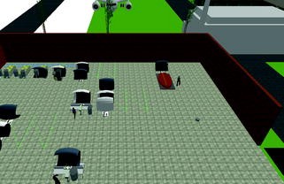
Snapshot of part of the 3D model.
-
2.
Due to an extra work requirement for a process.
-
3.
Due to an unfinished job (the shift ends and the work is not finished).
-
4.
Due to the correction work after the final test.

The job order is launched at determined time, but sometimes it cannot be executed because the server is busy/damaged, there is not aero structure to perform the job, the resources are not idle or there is no available worker. All the order launched that are not attended remain in stand by waiting to be attended.
An aero structure is only processed if the station is available, the required resources are ready and there are worker in the station. A worker can be in a station only if there is a job order that required him to go there.
When there is no problem all the job orders created in the input state (source 1) run smoothly because they always find workers and resources to perform their tasks. The problem occurs when sources 2, 3 and 4 start to create job orders that cannibalize the resources. Additionally, the availability of resources could decrease due break downs or programed maintenance, the same for the workers due to programed day-off and absences.
The simulation model includes a 3D view where the decision maker could follow the behavior of the system at different speeds and see how delivery delays begin to arise. He can see how the required variables are updating and where the aero structures, the transporter and the workers are in each moment. (See Fig. 4 for a Snapshot)

SMORE plot layout explanation.
Validation of the simulation model has occurred at two levels. Firstly, validation of the output results without any disruption or error against the optimization model and secondly, validation of the entire system model against real data from the plant.
4 Results
The experimentation was done in an Intel Core 7 with 8 GB of RAM, using Windows 10 and the discrete simulation software Simio Enterprise (2017).
We replicated each scenario 30 times; the results presented are the average of the replications. We tested the each option with the four scenarios described in Table 3.
Also, we evaluated 3 risk avoidance strategies for each scenario:
-
Baseline case, using the number of operator given in the detailed schedule.
-
Extra workers case, using one extra worker per early and late shift
-
Night workers case, using two extra operators per night shift.
In the results tables (Table 3), the first column is the scenario name that is composed of (Absence rate – Test Rejection – Type of risk avoidance strategy-Option A or B). The second column is the sum of all the delays (delivery hour – expected end). From the 3rd to the 6th column are the delivery hour of each aero structure. In the 7th column the on time deliver is the number of aero structures delivered before mid-day of the due day (96 + 12 = 108 h for this example). Finally, the 8th column is the mean number of failures that was caused due to machine failures and errors that require extra work.
The results have also been plotted using a SMORE (Simio Measure of Risk and Error) diagram. The layout of the plot is explained in Fig. 4. The SMORE plots (Fig. 4) have been built using a confidence interval of 95%, with a lower percentile of 25% and an upper percentile of 75%.

Confidence interval of Option A (Left) and Option B (Right)
In option A, it is interesting that the baseline case does not deliver more than one aero structure on time and zero in the more severe situation. The use of extra workers decreases the delay. It can be observed that the solution with extra workers presents better results as it can see in Fig. 5. The schedule is more robust against the variation of absence rate. In all the cases putting the extra workers during the night shift presents better results.
In a high rejection rate scenario, despite the improvement of the performance, neither adding operators during the early and late shift nor adding a night shift do we obtain a good performance. No option delivers more than 50% of the products on time in this scenario.
The baseline case of option B and the extra workers of option A, use the same number of workers and the option B delivers the double of units on time. The behavior of this schedule against the different scenarios was more stable due the extra number of workers. Not in all the cases the extra workers during the early and late shifts improve the result. The use of extra works during the night could deliver in the majority of the cases on time (incurring in the extra cost of the number of workers).
The effect of the failures is hard when the problems occur in certain process and moments. Analyzing the processing times, if we have 4 days, with 2 shifts we have 64 working hours. The time of the process equipping for FC-A-LH needs 60 h. Any problem or delay in this process will severely impact in the solution. Also, the number of workers during the week is constant, but when the absence of operators coincides with the day with a peak of work, its impact is higher.
Even though the rate of machine failures and errors that require extra work do not change from one scenario to another, they is not constant in all the runs due to the stochasticity of the model. The number of failures has an impact on the severity of the run. The difference of number of failures among the scenarios will decrease as we make more runs of each scenario.
5 Discussion
The deployment of PLM tools has provided relevant improvements in the aeronautical industry. One of its main aims is to enable the simulation of the whole manufacturing of the aircraft.
In this sense, discrete event simulation is an efficient tool for validating the production process design. It allows the identification of possible production process pitfalls at an early stage. It is also a useful tool not only for the preliminary design of the line but also for operative decision making during the production stage, for example, to asses the impact of changing for a faster or more reliable machine. In the short term planning it could help us to test contingency actions against disruptions such as planned and unplanned absences of workers, machine breakage and quality problems.
In this work, we have used a discrete event simulation model to asses the robustness of different schedules combined with three risk avoidance strategies. This kind of tests helps us to quantify better those expected real operating costs that are neglected otherwise. The results show that choosing the schedule with less planned workers leads to much higher late deliveries and therefore a higher real operating cost.
From the different strategies tested in this research, the night shift offers better response against the delays because the resources are not used and could help us to finish the entire unfinished task during the day. It is important to highlight, that only until the job order is launched the task could start. The job orders are launched as it was planned or to solve any problems, then they cannot advance work.
The importance of testing the robustness of the solution is better exemplified if we compare the Baseline Option A to Option B with extra workers. Baseline Option A delivers the double of units of time than Option B with extra workers. This is interesting since both use the same amount of workers during the shifts. The only difference is that in the Option B all the workers have assigned tasks, and help to solve the incidences when they can. In Option A, the original workers are over saturated with task, and the extra workers try to solve the incidences, which turns out to be a better policy.
As a future work we would like to extend the use of simulation to test the production process together with another processes of the plant, evaluating which option is better for each case. Another future research direction is to make further experimentation to create learned lessons such as the fact that the production scheduling with the minimum cost is not always the best solution.
References
Cunha, P.F., Mesquita, R.M.: The role of discrete event simulation in the improvement of manufacturing systems performance. In: Camarinha-Matos, L.M., Afsarmanesh, H. (eds.) Balanced Automation Systems II. IAICT, pp. 137–145. Springer, Boston, MA (1996). https://doi.org/10.1007/978-0-387-35065-3_13
Heike, G., Ramulu, M., Sorenson, E., Shanahan, P., Moinzadeh, K.: Mixed model assembly alternatives for low-volume manufacturing: the case of the aerospace industry. Int. J. Prod. Econ. 72(2), 103–120 (2001)
Herroelen, W., Leus, R.: Project scheduling under uncertainty: survey and research potentials. Eur. J. Oper. Res. 165, 289–306 (2005)
Jahangirian, M., Eldabi, T., Naseer, A., Stergioulas, L.K., Young, T.: Simulation in manufacturing and business: a review. Eur. J. Oper. Res. 203, 1–13 (2010)
Mas, F., Gómez, A., Menéndez, J.L., Ríos, J.: Proposal for the conceptual design of aeronautical final assembly lines based on the industrial digital mock-up concept. In: Bernard, A., Rivest, L., Dutta, D. (eds.) PLM 2013. IAICT, vol. 409, pp. 10–19. Springer, Heidelberg (2013). https://doi.org/10.1007/978-3-642-41501-2_2
Mas, F., Arista, R., Oliva, M., Hiebert, B., Gilkerson, I., Ríos, J.: A review of PLM impact on US and EU aerospace industry. Procedia Eng. 132, 1053–1060 (2015a)
Mas, F., Oliva, M., Ríos, J., Gómez, A., Olmos, V., García, J.A.: PLM based approach to the industrialization of aeronautical assemblies. Procedia Eng. 132, 1045–1052 (2015b)
Murphy, C.A., Perera, T.: The definition of simulation and its role within an aerospace company. Simul. Pract. Theory 9, 273–291 (2002)
Kadar, B., Pfeiffer, A., Monostori, L.: Discrete event simulation for supporting production planning and scheduling decisions in digital factories. In: Proceedings of the 37th CIRP International Seminar on Manufacturing Systems, pp. 444–448 (2004)
Leon, V.J., Wu, S.D., Storer, R.H.: Robustness measures and robust scheduling for job shops. IIE Trans. 26(5), 32–43 (1994)
Lu, H., Liu, X., Pang, W., Ye, W., Wei, B.: Modeling and simulation of aircraft assembly line based on quest. Adv. Mater. Res. 569, 666–669 (2012)
Noack, D., Rose, O.: A simulation based optimization algorithm for slack reduction and workforce scheduling. In: Proceedings of the 2008 Winter Simulation Conference, pp. 1989–1994 (2008)
Scott, H.A.: Modelling aircraft assembly operations. In: Proceedings of the 26th Conference on Winter Simulation, pp. 920–927 (1994)
Simio Enterprise [Computer software] Version 8.136. PA, USA: Simio LLC (2017)
Ziarnetzky, T., Mönch, L., Biele, A.: Simulation of low-volume mixed model assembly lines: modeling aspects and case study. In: Proceedings of the Winter Simulation Conference 2014 IEEE, pp. 2101–2112 (2014)
Author information
Authors and Affiliations
Corresponding author
Editor information
Editors and Affiliations
Rights and permissions
Copyright information
© 2017 IFIP International Federation for Information Processing
About this paper

Cite this paper
Pulido, R., Borreguero-Sanchidrián, T., García-Sánchez, A., Ortega-Mier, M. (2017). Analysis of the Robustness of Production Scheduling in Aeronautical Manufacturing Using Simulation: A Case Study. In: Ríos, J., Bernard, A., Bouras, A., Foufou, S. (eds) Product Lifecycle Management and the Industry of the Future. PLM 2017. IFIP Advances in Information and Communication Technology, vol 517. Springer, Cham. https://doi.org/10.1007/978-3-319-72905-3_16
Download citation
DOI: https://doi.org/10.1007/978-3-319-72905-3_16
Published:
Publisher Name: Springer, Cham
Print ISBN: 978-3-319-72904-6
Online ISBN: 978-3-319-72905-3
eBook Packages: Computer ScienceComputer Science (R0)