Abstract
Endoscopic videos have been widely used for stomach diagnoses. It is of particular importance to obtain the 3D shapes, which enables observations from different perspectives so as to facilitate comprehensive and accurate diagnoses. However, obtaining 3D shapes is challenging for traditional multi-view 3D reconstruction methods, due to strong motion blurs, reflections, low spatial resolutions, non-rigid surfaces, and limited view angle shifts. In this work, we propose a mesh regularization for shape recovery based on cues derived from Shape-from-Shading (SfS). We recover shapes for all frames to generate a 3D video. In particular, a 3D mesh is optimized for every frame according to the 3D raw data obtained from SfS. Although the raw data contains errors and temporal jitters, our spatially and temporally optimized meshes can well approximate the underlying non-rigid surfaces, rendering temporally-stabilized meshes for 3D video display. Our experiments demonstrate the effectiveness of our method on many challenging endoscopic videos.
You have full access to this open access chapter, Download conference paper PDF
Keywords
1 Introduction
Endoscopic videos have become the most reliable sources for observation and diagnosis of gastrointestinal hollow organs. Various gastrointestinal symptoms (such as inflammation, ulcers, and tumors) that cannot be diagnosed clinically or by other interventional examinations (such as abdominal ultrasound, barium meal, CT, and MRI) can be diagnosed by endoscopic approaches. Moreover, endoscopic treatments (such as bleeding termination, polyps-removing, structure dilation, abnormality removal, and removal of early cancer strippings) heavily rely on the endoscopic observations. However, 2D endoscopic image sequences taken by a common monocular endoscope lack 3D vision and depth perception. Enabling 3D vision can improve the accuracy of diagnosis and treatments.Footnote 1
The goal of our work is to recover the 3D shape of inner-surfaces as meshes for all frames of an endoscopic video, such that the traditional 2D video can be replaced by the 3D video that can be viewed from different 3D viewpoints, thus offering a flexible visualization for reliable diagnosis.
Our work is built upon Shape-from-Shading (SfS) for the 3D surface recovery. Okatani and Deguchi applied SfS to calculate 3D points based on different shading properties [1]. There are two assumptions in [1]: a single light source at the camera center and a Lambertian surface model. The former is naturally satisfied as most of the endoscopes have a central light for illumination, but the later is not always satisfied due to specular reflections from excretive liquid and liquid bubbles. Thus, the estimated 3D points at these regions are inaccurate or totally contaminated. We adopt a modified approach for 3D point clouds recovery by detecting these regions in the image and skipping their problematic 3D points during mesh optimization. In particular, we propose to constrain the mesh edge lengths (the length between neighboring mesh vertices) during mesh optimization. On one hand, the mesh is deformed obeying the SfS 3D points as data constraints. On the other hand, it is encouraged to maintain rigidities (e.g., a square mesh cell maintains the square shape after deformation). As a result, a non-linear system is formulated, which can be minimized efficiently via Gauss-Newton iterations.
We first recover the meshes for all frames independently. With regards to the temporal smoothness, we borrow the idea of the video stabilization method [2] to smooth meshes with a spatial-temporal optimization. As a result, the meshes not only represent the shape of underlying organ surfaces, but also vary smoothly to enable a vivid visualization.
2 Related Works
3D reconstruction methods are well documented in [3]. Sparse 3D points of a scene can be reconstructed if multiple views are provided. Multi-view stereo algorithms further upgrade sparse 3D points into dense 3D point clouds [4]. With regards to non-rigid shape reconstruction (recovery dynamic points from a single camera), some methods [5, 6] propose motion priors of the moving objects while others [7,8,9] adopt matrix factorization approaches. 3D models are more desired descriptions of structures compared to 3D point clouds. Various methods have been proposed to model different objects/structures, including facades [10], plants [11], hairs [12], and faces [13].
Mesh manipulations are utilized for 2D and 3D shape deformations. Igarashi et al. proposed “as-rigid-as-possible” mesh warping for 2D shape manipulations [14]. Some improvements have been made for detailed 2D shape preserving under large movements [15, 16]. 3D mesh deformations are utilized for 3D surface representations [17]. Sorkine et al. proposed a Laplacian surface editing method by enforcing coherence between neighboring mesh vertices [18]. How to maintain 3D details has been reported in [19, 20]. Our method is motivated by the content-preserving warps [21], where we manipulate quads in the 3D space for 3D organ surface representation.
Endoscopic modeling methods can be classified into two categories: Shape-from-Shading [1, 22, 23] and Structure-from-Motion (SfM) [24, 25]. Our method belongs to the first category. Though some assumptions of SfS are violated, our mesh deformation can compensate the inaccuracy and smooth the noise within SfS 3D points.
Our method is also related to video stabilization [2, 21, 26]. For this task, Liu et al. divided each video frame into a mesh and stabilized these meshes for stabilization [2]. We follow the similar idea to enforce the temporal smoothness of our surface meshes.
3 Our Method
In this section, we present our method for the 3D surface recovery. We first introduce a pre-processing, which provides the pruned SfS 3D point clouds. Then, we describe our method for mesh optimization.
3.1 Pre-processing
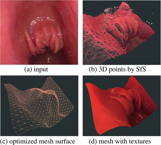
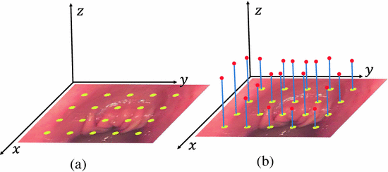
Endoscopic images usually contain many contaminated spots that violate the SfS assumptions, leading to problematic 3D points. In Fig. 1(a), we can observe many reflections due to gastric effusions. The recovered 3D points at these regions are inaccurate, as can be seen in Fig. 1(b). These reflection spots are detected by thresholding the image intensities. We then remove the 3D points that correspond to specular regions. Specifically, we sample points for every five pixels to produce our 3D raw data for the subsequent mesh optimization. The SfS calculation is based on [22]. Figure 2 shows an example of our setting. The yellow dots in Fig. 2(a) show the sampled control points that have zero height in the source frame. The heights of these control points are calculated according to SfS at the target frame (red dots in Fig. 2(b)). We want to place a 3D mesh on top of these control points to represent the 3D shape.
3.2 Mesh Optimization
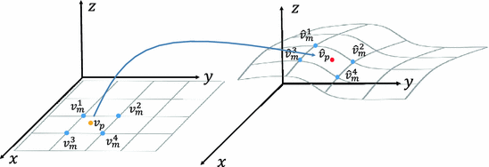
We define a uniform grid mesh as shown in Fig. 3(a). The control points are denoted as \(\{v_p,\hat{v}_p\}\), where \(v_p\) and \(\hat{v}_p\) denote the control points in the source and target mesh, respectively. The mesh vertices in the source and target frame are denoted as \(v_m\) and \(\hat{v}_m\), where the \(v_m\) is known, but \(\hat{v}_m\) needs to be solved. Notably, all the points are 3D vectors \((x,y,z)^T\). In the source frame, z values are zero.
Before and after mesh deformation. (a) The initialization is a flat source mesh. (b) The deformed target mesh is obtained by our optimization. The control point \(v_p\) in the source mesh can be represented by its enclosing four grid vertices \((v^1_m,v^2_m,v^3_m,v^4_m)\) using bilinear interpolation. We use the same weights to represent the control point \(\hat{v}_p\) in the target mesh by \((\hat{v}^1_m,\hat{v}^2_m,\hat{v}^3_m,\hat{v}^4_m)\).
The deformed mesh should satisfy both data constraints from control points [2] and smoothness constraints that maintain rigidity of mesh structures [16]. The proposed energy function is defined as:
where \(\alpha \) balances two terms, which is set to 1 in our implementation, and \(\hat{\mathbf{V }}_m\) represents the unknown mesh vertices.
Data constraints. In Fig. 3(a), the point \(v_p\) can be represented by its enclosing four vertices:
The same set of interpolation weights \((w^1_m,w^2_m,w^3_m,w^4_m)\) is used for representation of the point \(\hat{v}_p\) in the target mesh:
The data constraint is defined as:
where \(\hat{v}_{m_p}\) and \(w_p\) denote four vertices enclosing \(\hat{v}_p\) and the corresponding four interpolation weights, respectively. Equation (4) can be rewritten into matrix form:
where \(\mathbf W \) is an \(n{\times }m\) matrix with n equals to the number of the control points.
Smoothness constraints. We propose to constrain the edge lengths between adjacent vertices for the mesh rigidity. All edges from mesh cells produce an edge set \(\varOmega _e\). The energy function is defined as:
where \(e(\hat{\mathbf{V }}_{m_{i}},\hat{\mathbf{V }}_{m_{j}}) = \frac{\widetilde{l_{i,j}}}{l_{i,j}}(\hat{\mathbf{V }}_{m_{i}}-\hat{\mathbf{V }}_{m_{j}})\), \(l_{i,j}\) is the current length of edge between neighboring vertices \(\hat{v}_{m_i}\) and \(\hat{v}_{m_j}\), and \(\widetilde{l_{i,j}}\) is the original length. Likewise, Eq. (6) can be rewritten into matrix form:
where \(\mathbf L \) is a \(|\varOmega _e|{\times }m\) matrix and \(|\varOmega _e|\) denotes the number of edges. Bringing Eqs. (5) and (7) into Eq. (1), we have:
Optimizing the energy function in Eq. (8) gives the unknown mesh vertices \(\hat{\mathbf{V }}_m\). We set \(\alpha =1\) in our implementation.
Optimization. Equation (8) can be reformulated as:
where
Note that both \(\mathbf A \) and \({\hat{\mathbf{V }}_{p}}\) can be determined beforehand and are fixed during deformation, while \(\mathbf b \) is dependent on the current point positions \(\hat{\mathbf{V }}_{m}\). Therefore, this is a nonlinear least squares problem. We utilize an iterative Gauss-Newton method [27] in which Eq. (9) is interpreted as:
where \(\hat{\mathbf{V }}^{k}_{m}\) is the vertex positions solved from the k-th iteration and \(\hat{\mathbf{V }}^{k+1}_{m}\) is to be solved at the iteration \(k+1\), respectively. Given that \(\mathbf b (\hat{\mathbf{V }}^{k}_{m})\) is known at the current iteration, Eq. (11) can be solved by a standard linear least square solver:
We update \(\mathbf b (\hat{\mathbf{V }}^{k}_{m})\) during each iteration until \(\hat{\mathbf{V }}_{m}\) converges to a relatively stable matrix. Namely, we need to update \(e(\hat{\mathbf{V }}^{k}_{m})\) according to:
Empirically, 3–4 iterations converge to a stable solution (Fig. 4).
Smoothing of recovered meshes. At frame t, a homography \(F_i(t)\) for the cell i is estimated between adjacent mesh cells using 8 corresponding mesh vertices. The smoothing is conducted by a spatial-temporal optimization [2].
3.3 Temporal Smoothness
So far, we have presented the solution for mesh deformation at each frame, where the temporal smoothness has not yet been considered. The 3D raw data from SfS not only contains noises in spatial but also jitters in temporal. Therefore, we propose to filter the mesh vertices after all meshes being solved. We notice that the video stabilization method [2] fits well to this case and thus is adopted here for the spatial-temporal meshes smoothing.
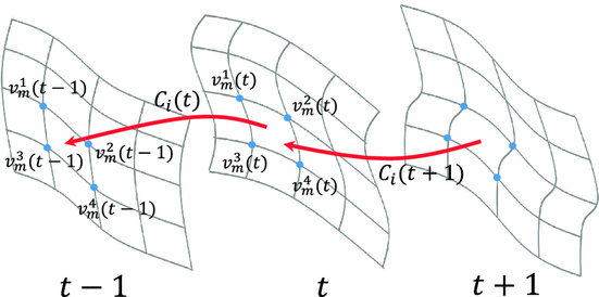
Figure 5 shows the configuration after obtaining meshes for all frames. At time t, a local homography \(F_i(t)\) of a cell i is estimated using 8 corresponding cell vertices, namely, \(\{v_m^1(t),v_m^2(t),v_m^3(t),v_m^4(t)\}\) and \(\{v_m^1(t-1),v_m^2(t-1),v_m^3(t-1),v_m^4(t-1)\}\). We estimate \(F_i\) for all frames and for mesh cells. Chaining all \(F_i\) for cell i of all frames defines a local path:
where \(C_i(t)\) is often referred to as a camera path in the context of video stabilization. Optimizing the following energy function gives the smoothed local path \(P_i\):
where \(\varPhi _t\) denotes the neighborhood at frame t and N(i) includes eight neighbors of the grid cell i.
The first term smooths local paths while the second one enforces spatial similarities of local paths. Equation (15) is quadratic and can be minimized efficiently by linear system solvers. A local update transform \(B_i(t)\) (\(B_i(t) = C_i(t)P(t)\)) is obtained for each cell. Applying \(B_i(t)\) to the corresponding vertices leads them to the smoothed positions. Each vertex receives four smoothed positions as it is shared by four cells (boundary vertices have fewer smoothed positions). For a vertex, we take the average of these positions to get its final position.
4 Results
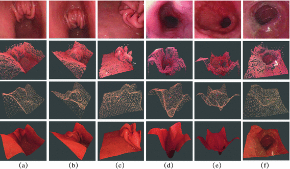
We implemented our system using C++. We run our method on a laptop with Intel i7-5500U 2.4 GHz Core(TM) and 8 GB RAM. It takes only 1 s to reconstruct a frame, in which SfS, mesh optimization, and smoothing take 0.2, 0.7, and 0.1 s, respectively. The input image has resolution of \(306\times 370\) pixels. The mesh resolution is \(32\times 32\). Some results are presented in Fig. 5. Each column shows an example where the original frame, SfS 3D points, optimized mesh, and the final textured results are placed on each row.
Note that Examples (a) and (b) are different frames from the same endoscopic video, and so are Examples (d) and (e). Our optimization manipulates mesh quads, but we draw a quad into two triangles for a clear illustration. We can view the 3D structures under different perspectives. Here, only one perspective is selected for each example due to the limited space. Please refer to our supplementary file for the 3D videos of these examples as well as other results. In our experiments, some examples contain tissues moving outwards (Fig. 5(a), (b), and (c)) and some examples contain hollow pipes (Fig. 5(d), (e), and (f)). Our reconstructed shapes can represent all these structures faithfully.
Lastly, we would like to state that our recovered 3D shape is not a metric 3D reconstruction, because SfS itself is not a metric reconstruction and the stabilization changes the values of vertices non-physically. Moreover, it is challenging to obtain ground-truth data so as to conduct a quantitative evaluation. Our goal in this work is to grab the shapes of the underlying real surfaces and deliver a flexible 3D view for a clearer visualization.
5 Conclusions
We have presented a method to recover the inner-surface’s shape of organs from endoscopic videos. Specifically, we compute 3D raw point clouds from SfS and optimized a mesh to fit to these point clouds to represent the shape of underlying surfaces. We deform a mesh for each frame. All meshes of frames are stabilized by a spatial-temporal optimization for the temporal smoothness. As a result, a 3D video is generated which can be viewed under different viewpoints. Various challenging examples validate the effectiveness of our proposed method.
Notes
- 1.
Supplementary: http://www.liushuaicheng.org/ICIG/2017/SuppEndoscopic.mp4.
References
Okatani, T., Deguchi, K.: Shape reconstruction from an endoscope image by shape from shading technique for a point light source at the projection center. Comput. Vis. Imag. Under. 66(2), 119–131 (1997)
Liu, S., Yuan, L., Tan, P., Sun, J.: Bundled camera paths for video stabilization. ACM Trans. Graph. 32(4), 78 (2013)
Hartley, R., Zisserman, A.: Multiple View Geometry in Computer Vision, 2nd edn. Cambridge University Press, New York (2003)
Seitz, S., Curless, B., Diebel, J., Scharstein, D., Szeliski, R.: A comparison and evaluation of multi-view stereo reconstruction algorithms. In: Proceedings of CVPR (2006)
Bregler, C., Hertzman, A., Biermann, H.: Recovering non-rigid 3D shape from image streams. In: Proceedings of CVPR (2000)
Liu, S., Wang, J., Cho, S., Tan, P.: TrackCam: 3D-aware tracking shots from consumer video. ACM Trans. Graph. 33(6), 198 (2014)
Lee, S., Park, K., Kim, J.: A SfM-based 3D face reconstruction method robust to self-occlusion by using a shape conversion matrix. Pattern Recogn. 44(7), 1470–1486 (2011)
Tomasi, C., Kanade, T.: Shape and motion from image streams under orthography: a factorization method. Int. J. Comput. Vis. 9(2), 137–154 (1992)
Yan, J., Pollefeys, M.: A factorization-based approach to articulated motion recovery. In: Proceedings of CVPR (2005)
Xiao, J., Fang, T., Tan, P., Zhao, P., Ofek, E., Quan, L.: Image-based facade modeling. ACM Trans. Graph. (TOG) 27(5), 161 (2008). (Proc. of SIGGRAPH Asia)
Quan, L., Tan, P., Zeng, G., Yuan, L., Wang, J., Kang, S.: Image-based plant modeling. ACM Trans. Graph. (TOG) 25(3), 599–604 (2006). (Proc. of SIGGRAPH)
Wei, Y., Ofek, E., Quan, L., Shum, H.-Y.: Modeling hair from multiple views. ACM Trans. Graph. (TOG) 24, 816–820 (2005)
Ira, K.-S., Basri, R.: 3D face reconstruction from a single image using a single reference face shape. IEEE Trans. Pattern Anal. Mach. Intell. 33(2), 394–405 (2011)
Igarashi, T., Moscovich, T., Hughes, J.: As-rigid-as-possible shape manipulation. ACM Trans. Graph. 24(3), 1134–1141 (2005)
Schaefer, S., McPhail, T., Warren, J.: Image deformation using moving least squares. ACM Trans. Graph. 25, 533–540 (2006)
Weng, Y., Xu, W., Wu, Y., Zhou, K., Guo, B.: 2D shape deformation using nonlinear least squares optimization. The Vis. Comput. 22(9–11), 653–660 (2006)
Botsch, M., Sorkine, O.: On linear variational surface deformation methods. IEEE Trans. Vis. Comput. Graph. 14(1), 213–230 (2008)
Sorkine, O., Cohen-Or, D., Lipman, Y., Alexa, M., Rössl, C., Seidel, H.-P.: Laplacian surface editing. In: Proceedings of Eurographics, pp. 175–184 (2004)
Zhou, K., Huang, J., Snyder, J., Liu, X., Bao, H., Guo, B., Shum, H.-Y.: Large mesh deformation using the volumetric graph Laplacian. ACM Trans. Graph. 24, 496–503 (2005)
Lipman, Y., Sorkine, O., Levin, D., Cohen-Or, D.: Linear rotation-invariant coordinates for meshes. ACM Trans. Graph. 24, 479–487 (2005)
Liu, F., Gleicher, M., Jin, H., Agarwala, A.: Content-preserving warps for 3D video stabilization. ACM Trans. Graph. 28, 44 (2009)
Forster, C., Tozzi, C.: Towards 3D reconstruction of endoscope images using shape from shading. In: Proceedings of Computer Graphics and Image Processing, pp. 90–96 (2000)
Wang, G., Han, J., Zhang, X.: Three-dimensional reconstruction of endoscope images by a fast shape from shading method. Meas. Sci. Technol. 20(12), 125801 (2009)
Yang, B., Zhou, Y., Hu, X., Lin, J., Xing, Q.: Optical-tracker-based 3D reconstruction for endoscopic environment. App. Mechan. Materi. 249, 1277–1282 (2013)
Thormahlen, T., Broszio, H., Meier, P.: Three-dimensional endoscopy. In: Falk Symposium, pp. 199–214 (2002)
Liu, S., Tan, P., Yuan, L., Sun, J., Zeng, B.: MeshFlow: minimum latency online video stabilization. In: Proceedings of ECCV, pp. 800–815 (2016)
Madsen, K., Bruun, H., Tingleff, O.: Methods for non-linear least squares problems (1999)
Acknowledgements
This work has been supported by National Natural Science Foundation of China (61502079 and 61370148).
Author information
Authors and Affiliations
Corresponding author
Editor information
Editors and Affiliations
Rights and permissions
Copyright information
© 2017 Springer International Publishing AG
About this paper
Cite this paper
Ren, Z., He, T., Peng, L., Liu, S., Zhu, S., Zeng, B. (2017). Shape Recovery of Endoscopic Videos by Shape from Shading Using Mesh Regularization. In: Zhao, Y., Kong, X., Taubman, D. (eds) Image and Graphics. ICIG 2017. Lecture Notes in Computer Science(), vol 10668. Springer, Cham. https://doi.org/10.1007/978-3-319-71598-8_19
Download citation
DOI: https://doi.org/10.1007/978-3-319-71598-8_19
Published:
Publisher Name: Springer, Cham
Print ISBN: 978-3-319-71597-1
Online ISBN: 978-3-319-71598-8
eBook Packages: Computer ScienceComputer Science (R0)


